City, University of London Institutional Repository
Citation
:
Phillips, J. P., Kyriacou, P. A. & Jones, D. P. (2010). Calculation of Photon Path
Changes due to Scatter in Monte Carlo Simulations. Conference proceedings : ... Annual
International Conference of the IEEE Engineering in Medicine and Biology Society. IEEE
Engineering in Medicine and Biology Society. Conference, pp. 4959-4962. doi:
10.1109/IEMBS.2010.5627216 ISSN 1557-170X
This is the accepted version of the paper.
This version of the publication may differ from the final published
version.
Permanent repository link: http://openaccess.city.ac.uk/13344/
Link to published version
:
http://dx.doi.org/10.1109/IEMBS.2010.5627216
Copyright and reuse:
City Research Online aims to make research
outputs of City, University of London available to a wider audience.
Copyright and Moral Rights remain with the author(s) and/or copyright
holders. URLs from City Research Online may be freely distributed and
linked to.
City Research Online:
http://openaccess.city.ac.uk/
[email protected]
Justin P. Phillips,
Member, IEEE
, Panayiotis A. Kyriacou,
Senior Member, IEEE
, Deric P Jones,
Senior
Member, IEEE
.
Abstract— Computation using Monte Carlo simulations is widely used for modelling the light-tissue interaction. Despite this, many of the methods used for building such simulations are poorly described in the literature. In particular, a scheme for translating the scatter angles produced from a phase function into updated photon direction vectors is not explicitly reported. To address this, a method for calculating the change in photon direction following a scattering event is described, thus illuminating one of the fundamental ‘building blocks’ for researchers developing their own Monte Carlo models. The equations derived in this paper may be readily incorporated into applicable Monte Carlo program code.
I. INTRODUCTION
Monte Carlo simulation is a type of computational algorithm that uses repeated random sampling to compute its results. Monte Carlo simulations are often used to model physical systems that are too complicated or too poorly understood to allow computation of an exact result using analytical methods. Monte Carlo simulations rely on a large number of repeated calculations on random (or pseudo-random) input. Results from a Monte Carlo model have been compared with diffusion theory using optical interaction coefficients typical of mammalian soft tissues in the red and near infrared regions of the spectrum [1]. A Monte Carlo model for multi-layered media coded in the C computer language was described by Wang et. al. in 1995. The simulation program allows the user to specify the number of layers, the thickness of each layer as well as the absorption and scattering properties of each layer [2].
In the present study, a Monte Carlo simulation program was implemented that incorporates the scheme for translating the scatter angles into updated photon direction vectors and is described in this paper. Sample results of a simple single-layer tissue model are presented to demonstrate that the model gives reasonable results, which may be compared to independently derived experimental or theoretical results.
Consider a collimated monochromatic beam of light normally incident on the surface of a semi-infinite slab of homogeneous tissue. Each individual photon enters the tissue and most likely undergoes a number of
Manuscript received April 23, 2010.
J. P. Phillips and P.A. Kyriacou and D. P. Jones are with the School of Engineering and Mathematical Sciences, City University, London, EC1V 0HB, UK (e-mail: [email protected]).
scattering events before either being absorbed within the tissue or re-emitted at the surface of the slab. The scatter coefficient (s) is defined as the number of scattering events per unit distance travelled by a photon within the medium. After each scatter, the photon’s path deviates from its original direction by the scatter angle . The new position of the photon also depends upon the rotational azimuth scatter angle, as shown in Figure 1.
Fig. 1 A single scattering event. The resulting photon trajectory depends upon the scatter angle and the azimuth scatter angle
Scattering in biological media is usually considered anisotropic, i.e. the angle of scatter produced at each scattering event is not equally probable for all angles. Scattering media such as tissue may be described in terms of the absorption and scatter coefficients as well as a third variable, g, the anisotropic scattering factor, equal to the average cosine of caused by a large number of scattering events. If g = 0, the photons would undergo totally isotropic scattering, whereas the case where g = 1 would result in a scatter angle of zero, i.e. the photon would not change direction at all. For tissue, g is usually between 0.85 and 0.99, implying that small angle scattering is favoured [1, 2].
For multiple scattering events, the distribution of scatter angles is governed by a phase function. The most widely used of these is the Henyey-Greenstein phase function, which was originally derived to explain scattering phenomena in interstellar gas clouds but has since been widely applied to modelling of the light-tissue interaction [3, 4]:
P hg(cos) 1 2
(1g2)
(12gcos g2)3 2 (1) [5]. For values of g in the tissue range, small angles of scatter, i.e. values of cos(close to 1, are much more probable than large angles. Any absorbing and scattering medium can thus be characterised by the variables, a, s, and g. The mean path length of a photon before
Calculation of Photon Path Changes due to Scatter in
Monte Carlo Simulations
absorption is 1/a, the mean free–path distance between scattering events is 1/s and the mean angle of scatter for all scattering events is cos-1(g).
II. MATERIALS AND METHODS
A. Implementation of the model
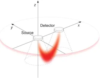
[image:3.612.88.256.273.404.2]A Monte Carlo model, subsequently referred to as the MCM, was created to model light transport through tissue illuminated by a reflectance probe of the type used in NIRS systems [6] as shown in Figure 2. It was supposed that a semi-infinite slab of tissue is illuminated by a disc-shaped source of optical radiation, whose axis lies along the z-axis, placed on the tissue surface so that the coordinates of the centre of the source are (0, 0, 0). A circular detector is also placed on the surface a distance s along the x-axis so that the coordinates of the detector centre are (s, 0, 0).
Fig. 2 Geometrical arrangement of source, sensor and tissue as used in the Monte Carlo model (MCM). The origin of the coordinate system is the centre of the light source.
The tissue was treated as a single layer of a homogenous scattering and absorbing medium and the tissue boundary is defined by the plane z = 0. The optical properties of the tissue for the incident wavelength must be accounted for in the model as well as other variables such as the emitter and detector diameters and numerical apertures.
B. Execution of the MCM
When the MCM is executed, a ‘virtual’ photon is launched into the tissue from the emitter. The initial position and direction of this photon is randomised but constrained by the limits imposed by the emitter radius (r) and its numerical aperture (NA). The initial position of the photon (x, y, z) is in a randomly generated position but constrained to the face of the circular emitter. The value of z is therefore initially 0, while, x and y values are randomly chosen such that x2 + y2 < r2. The direction of travel of the photon is defined using the two spherical angles, and , where (the zenith angle) is the angle between the photon’s direction vector and the positive z -axis and (the azimuth angle) is the angle between the projection of the direction vector onto the x-y plane and the positive x-axis respectively. It is assumed that any exit
angle within the cone of emission is equally probable, so the zenith angle, is assigned an initial value given by
=2
emm
(2)where is a uniformly distributed random number between 0 and 1, and
emmsin1(NA)
.
(3)A random number is initially assigned to the azimuth angle thus
= 2
.
(4)The photon free-path step size l, i.e. the distance to the next scatter, is then calculated using the following method. It is assumed that the free-path step size of the photon can have any value (i.e. 0 < l < ∞). It can be shown that the probability of a photon undergoing a scattering event whilst travelling a small distance dl’ after travelling a given distance l’ through a scattering medium is
p
s[
l
]
se
sl
(5)
[7]. The cumulative probability function, i.e. the probability of a scatter occurring whilst the photon is travelling a distance l through the tissue, is found by integrating Equation 5 between 0 and l:
P
s[l]
s0
l
e
sl d
l
1
e
sl(6)
Note that
P
s
1 as
l
. This probability function is sampled using computer-generated random numbers, to generate values of l.The scatter angle is then calculated, which is the angle at which the photon leaves the point of scatter (before travelling a distance l to the next scatter) using the Henyey-Greenstein probability density function (Equation 1). The procedure is the same as that described above for generating the photon step size, l. For a given scattering event, the variable cos( falls with probability
P hg(cos) d(cos)within the interval [cos , cos + d(cos)]. The cumulative probability distribution, obtained from the integral of
P
hg(cos
) d(cos
)
may be sampled using the random variable thus
P
hg(cos
)
1 cos
d(cos
)
. (7)
cos
1
2
g
1
g
2
1
g
21
g
2
g
2
(8)[4]. The azimuth scatter angle is assigned a random angle between 0 and 2π radians, i.e.
2
. (9)C. Calculation of new photon direction after a scattering event.
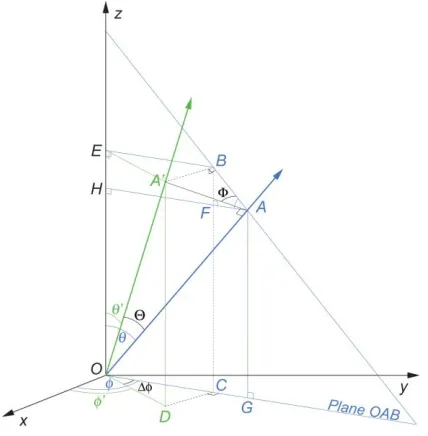
Since each scattering event causes a change in the direction of the photon, new values of the spherical angles defining the photon’s direction of travel with respect to the original axes must be calculated after each scatter. The zenith and azimuth angles defining the new direction of travel, ’ and ’ respectively, may be calculated from the original direction (defined by and and the scatter angles (and . A convention was established whereby the scatter azimuth angle is measured from the plane containing the z-axis and the original direction vector.
The method of calculating the direction of travel of a photon after a scattering event as used in the Monte Carlo model MCM program is given thus. Consider a photon travelling in the direction of vector OA, scattered in the direction of OA’ by a particle at O. Figure 3 shows a diagram of an example of original direction vector OA and a new direction vector OA’ drawn in three dimensions. The distance of A’ from O is arbitrarily chosen.
Fig. 3. Diagram of example direction vectors, drawn in three dimensions, of a photon before and after scatter (vectors OA and OA’
respectively) by a particle at point O.
The azimuth scatter angle may be measured from any zero value, since all angles of are equally probable. For convenience is measured from the plane containing the z-axis and OA. Point B is the point in this plane closest to A’, i.e. A’B is perpendicular to the plane. The cosine of the new zenith angle ’ is given by the ratio of the projection of OA’ on the z-axis and OA’:
cos
EOOA (10)
where EO = EH + OH
.
Note that the position of point A is chosen so that OAA’ is a right angle. Also note that lines OH and OE are the projections onto the z-axis of OA and OA’ respectively. Points G and C are points of intersection of vertical lines dropped from A and B respectively onto the x-y plane. Point F is the point of intersection of AH and BC.So, EOABsin
OAcos
(11) EOAAcossin
OAcoscos
(12) EOOA'sincossin
OAcoscos
(13) from Equation 10:cos
sincossin
coscos
. (14)The change in the azimuth angle caused by the scattering (∆is found from the following relation:
tan
CDOC
A B OGCG
AAsin
OAsin
ABcos
(15) so, tan
OA'sinsinOAcossin
AAcoscos
(16) therefore,tan
OAsinsinOAcossin
OAsincoscos
(17) therefore,tan
sinsincossin
sincoscos
. (18)D. Photon propagation, absorption and detection After each scattering event, the probability of the photon being absorbed is calculated from a cumulative probability distribution derived from Beer’s law [8] for the calculated free-path length l:
[image:4.612.53.267.450.668.2]and the photon randomly terminated according to this probability. If the photon survives, a check is made to see if the photon has fulfilled the detection criteria, i.e. the photon must arrive at the tip of detector within its cone of acceptance. If so, several variables are recorded including the photon’s path, total path length and the maximum depth of penetration into the tissue. If the photon is ‘lost’ (i.e. if it is absorbed, exits the tissue at the surface or the photon strikes the detector fibre at an angle greater than the acceptance angle) the photon path information is discarded.
E. Demonstration of the MCM
The single-layer MCM program described above was implemented in LabVIEW MathScript Version 8.5 running on an iMac computer (Apple Inc., Cupertino, CA, USA) with a 2.4 GHz Intel dual-core processor. The separation between the emitter and detector was set to 3 cm and the emitter and detector diameters were both 5 mm. The numerical aperture of the source and the detector was set to 0.39. The absorption coefficient of the tissue a was set to 0.01 mm-1 and the anisotropy factor g set to 0.99. Results for two values of the scatter coefficient s were compared: 2.0 mm-1 and 5.0 mm-1. In each case the simulation was run until 4000 virtual photons had been detected.
III. RESULTS
The mean (±SD) optical path of the 4000 photons was found to be 86.9 ± 45.9 mm when s = 2 mm-1 and 76.2 ± 40.9 mm when s = 5 mm-1. Figure 4(a) shows a histogram of the distribution of optical path lengths of the detected photons for each of the two values of s. The lower scatter coefficient causes the photons to take a longer mean path through the tissue when travelling from the source to the detector.
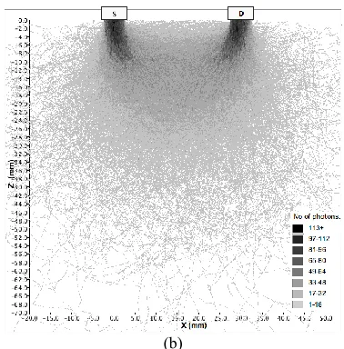
Figure 4(b) shows a density plot of photon scatters for detected photons in the case where s= 5 mm-1. The photon paths in three dimensions are shown projected onto a 2-d (X-Z) plane. It can be seen that there is a high concentration of photons near the source and the detector. Some photons appear to penetrate into the illuminated medium deeply while others take a more direct route from source to detector.
(a)
[image:5.612.346.535.63.255.2](b)
Fig. 4 (a) Distribution of optical path lengths for detected photons; n=4000. (b) density plot of photon scatters for detected photons;n=4000, s= 5 mm-1.
IV. CONCLUSION
In the demonstration example, the MCM predicted that in a uniform homogenous scattering medium, the optical path of photons travelling from a source to an adjacent detector is dependent on the scatter coefficient. At lower scatter coefficients, the photons travel further into the tissue before being scattered sufficiently to return to the detector.
A practical Monte Carlo model was described in the paper. The techniques described, in particular Equations 14 and 18, may be usefully incorporated into computer programs. Much MCM programs may be utilised in a wide variety of applications for predicting the behaviour of photons in tissue.
REFERENCES
[1] Yaroslavsky AN, Schulze PC, Yaroslavsky IV, Schober R, Ulrich F, Schwarzmaier HJ. Optical properties of selected native and coagulated human brain tissues in vitro in the visible and near infrared spectral range. Physics in Medicine & Biology 2002;47(12):2059-73.
[2] Meinke M, Muller G, Helfmann J, Friebel M. Empirical model functions to calculate hematocrit-dependent optical properties of human blood. Applied Optics 2007;46(10):1742-53.
[3] Hestenes K, Nielsen KP, Zhao L, Stamnes JJ, Stamnes K. Monte Carlo and discrete-ordinate simulations of spectral radiances in a coupled air-tissue system. Applied Optics 2007;46(12):2333-50. [4] Binzoni T, Leung TS, Gandjbakhche AH, Rufenacht D, Delpy DT. The use of the Henyey-Greenstein phase function in Monte Carlo simulations in biomedical optics.[see comment]. Physics in Medicine & Biology 2006;51(17):N313-22.
[5] Witt AN. Multiple scattering in reflection nebulae: I. A Monte Carlo approach Astrophys J 1977;35: S1–6.
[6] Phillips JP, Langford RM, Jones DP. Investigation of an optical fiber cerebral oximeter using a Monte Carlo model. Conference Proceedings: Annual International Conference of the IEEE Engineering in Medicine & Biology Society 2007;2007:1113-6.
[7] Wang L, Jacques SL, Zheng L. MCML--Monte Carlo modeling of light transport in multi-layered tissues. Computer Methods & Programs in Biomedicine 1995;47(2):131-46.
[image:5.612.54.289.587.731.2]