City, University of London Institutional Repository
Citation:
Nomikos, N. and Soldatos, O. A. (2010). Analysis of model implied volatility for jump diffusion models: Empirical evidence from the Nordpool market. Energy Economics, 32(2), pp. 302-312. doi: 10.1016/j.eneco.2009.10.011This is the accepted version of the paper.
This version of the publication may differ from the final published
version.
Permanent repository link:
http://openaccess.city.ac.uk/7527/Link to published version:
http://dx.doi.org/10.1016/j.eneco.2009.10.011Copyright and reuse: City Research Online aims to make research
outputs of City, University of London available to a wider audience.
Copyright and Moral Rights remain with the author(s) and/or copyright
holders. URLs from City Research Online may be freely distributed and
linked to.
City Research Online: http://openaccess.city.ac.uk/ [email protected]
Analysis of Model Implied Volatility for Jump Diffusion Models:
Empirical Evidence from the Nordpool Market
Nikos K Nomikos*
and
Orestes A Soldatos**
ABSTRACT
In this paper we examine the importance of mean reversion and spikes in the stochastic behaviour of the underlying asset when pricing options on power. We propose a model that is flexible in its formulation and captures the stylized features of power prices in a parsimonious way. The main feature of the model is that it incorporates two different speeds of mean reversion to capture the differences in price behaviour between normal and spiky periods. We derive semi-closed form solutions for European option prices using transform analysis and then examine the properties of the implied volatilities that the model generates. We find that the presence of jumps generates prominent volatility skews which depend on the sign of the mean jump size. We also show that mean reversion reduces the volatility smile as time to maturity increases. In addition, mean reversion induces volatility skews particularly for ITM options, even in the absence of jumps. Finally, jump size volatility and jump intensity mainly affect the kurtosis and thus the curvature of the smile with the former having a more important role in making the volatility smile more pronounced and thus increasing the kurtosis of the underlying price distribution.
Keywords: Affine Jump Diffusion Model, Implied Volatility, Volatility Skew, Electricity Derivatives, Risk Management
JEL Classification: G13, G12 and G33
Acknowledgements: We are grateful to Derek Bunn and John Hatgioannides for suggesting useful improvements.
* Corresponding Author: Faculty of Finance, Cass Business School, London EC1Y 8TZ, UK. email: [email protected]; tel: +44 207040 0104: fax: +44 207040 8681
** Research, Total Gas & Power Ltd, London E14 5BF, UK.
1 Introduction
Over the last 10 years radical changes have taken place in the structure of electricity markets around the world. Following the deregulation of power markets, prices are now determined under the fundamental rule of supply and demand and the resulting price volatility has increased the need for risk management using derivative contracts such as futures and options. It is important therefore for market participants to use option pricing models that can price fairly the most significant risks that exist in the market. However, due to the unique features of power markets, the traditional approaches for the pricing of derivatives that are used in other financial and commodity markets are not applicable to electricity. For instance, electricity is a non-storable commodity and a non-tradable asset which implies that arbitrage across time and space is limited. In addition, electricity prices exhibit extreme movements and volatility over short periods of time and are characterised by spikes which occur due to short-term supply shocks. Given these features of power prices, the assumption used in the Black-Scholes-Merton (BSM) model (Black and Scholes, 1973 and Merton, 1973) that the underlying asset follows a log-normal random walk, may not be appropriate.
The issue of modelling power prices has been investigated extensively in the literature. For instance, Lucia and Schwartz (2002) use a mean reverting process, as in Vasicek (1977), and a two-factor model, along the lines of Schwartz and Smith (2000), to model power prices in Nordpool. Villaplana (2003) introduces a two-factor jump-diffusion model and shows the significance of jumps in explaining the seasonal forward premium in the market. Bessembinder and Lemmon (2001) and Longstaff and Wang (2002) show that the sign and size of the forward premium is related to economic risks and the willingness of market participants to bear those risks. Geman and Roncoroni (2006) introduce a marked-point process calibrated to capture the trajectoral and statistical features of power prices. Weron (2008) models Nord Pool prices using a jump diffusion model and Nomikos and Soldatos (2008) apply a seasonal affine jump diffusion model with regime switching in the long-run equilibrium level to model spot and forward prices in the same market.
incorporates two different speeds of mean reversion - one for the diffusive part of the model and another one for the spikes - in order to capture the spiky behaviour of jumps and the slower mean reversion of the diffusive part of the model. Spikes are short-lived price movements of the spot market that do not spill-over to the forward market and, as such, they mean-revert at a much faster speed than ordinary shocks in the market. The proposed model is flexible in its formulation and encompasses the stylised features of many of the deregulated electricity markets around the world, as these have been identified in the literature. Therefore, although the model is calibrated to the Nordpool market, our results apply in general to other power markets as well.
The performance of the spike option pricing model is assessed empirically on the basis of the model implied volatilities that it generates; that is, the implied volatilities for which the option price from the BSM model matches the price from the proposed spike model. Model implied volatilities provide a very useful framework for assessing the performance of option pricing models as they illustrate the volatility shape and term structure that a model can theoretically capture in the market. The use of model implied volatilities is also justified by the fact that the market for exchange traded options in power is not liquid and thus, we cannot rely on traded option prices to assess the fit of the model in the market. The analysis of model implied volatilities has received little attention in the options pricing literature for the power markets, although the same methodology has been applied for instance in the equity options markets by Branger (2004) who compares model implied volatilities generated using Merton’s (1976) jump diffusion and Heston’s (1993) stochastic volatility models. In fact, the proposed methodology can be applied to markets for which liquid option markets do not exist but, the pricing of options, for either over-the-counter trading or for real options applications, is important and thus, one wants to test the validity and properties of alternative option pricing models.
implied volatilities, we derive semi-closed form solutions for European options based on the spike model, using the transform analysis by Duffie et al (2000). Our results indicate that the volatility skew depends primarily on the size and sign of the spikes whereas, it is the jump size volatility - rather than the jump intensity - that plays more important role in making the volatility smile more pronounced and thus increasing the kurtosis of the price distribution. Furthermore, even in the absence of spikes, we find that implied volatilities exhibit skewness since mean reversion does not allow the underlying prices to reach very high or low price levels, thus reducing the probability of an out-of-the-money option ending in-the-money
The structure of this paper is as follows: the following section reviews the theory of option pricing and derives semi-closed form solutions for the spike model. In section 3 we derive the theoretical moments of the risk neutral distribution of the spike model. Section 4 presents the model implied volatilities generated by the model using different model parameters each time and providing intuitive explanations in terms of the moments of the underlying price distribution. Finally, Section 5 concludes the paper.
2 Options Pricing using the spike model
Modelling electricity prices presents a number of challenges for researchers for a number of reasons. Power prices tend to fluctuate around values determined by the marginal cost of generating electricity and the level of demand, in other words they have a tendency of mean
reversion to an equilibrium price, which is a common feature of most commodity markets.
Power prices also tend to change by the time of day, week or month and in response to cyclical fluctuations in demand, and thus contain a seasonality component. In addition, the
non-storability of electricity means that inventories cannot be used to smooth-out temporal
supply-demand imbalances which results in high volatility. This, coupled with supply-side shocks such as generating or transmission constraints and unexpected outages, cause temporary price “spikes” due to restrictions in the available capacity which may take from a
will enter the market to take advantage of the higher price thus forcing the price to revert back to its long-run mean. There is also another implication of the convex shape of the supply stack; at higher price levels the supply stack curve becomes steeper and steeper, hence price changes are bigger for a given change in demand, causing an asymmetry in the volatility. This is exactly the opposite from what is noticed in the equity markets, and is known as the inverse
leverage effect (see e.g. Geman, 2005).
Therefore, electricity prices have the tendency to mean-revert to an equilibrium level which also implies a decreasing volatility term structure as time to maturity increases. This phenomenon, known as the Samuelson effect (1965), is due to the fact that for non-storable commodities, such as electricity, any new information in the market will have a more prominent effect on derivative prices that are closer to maturity. Electricity prices also exhibit very high volatility, where spikes play a major role. In general, when spikes occur they do not spill over to the forward market, since they are short lived. (Geman, 2005) On the other hand, the existence of spikes induces excess skewness and kurtosis to the distribution of spot electricity prices, and this also has a direct impact on option prices, especially for out-of-the-money (OTM) call options which now have higher probability of ending in-the-out-of-the-money (ITM), compared to the BSM model. This is also what causes the implied volatility from market prices in the BSM model not to be constant across strike prices but to have a smile or smirk shape as it will be shown in the next section.
These properties of power prices can be captured by the seasonal spike mean-reverting model where the spot price, Pt, is modelled as the sum of a deterministic seasonal component, f(t),
and the exponential sum of a stochastic component, Xt , which follows a stationary (as in
Vasicek, 1977) process reverting to an equilibrium value, and a spike factor, Y, as follows:
1
2
2
* ( ) exp(
( )
)
(
,
)
t t t
t t X
t t J J
X X
P f t X Y
dX k X dt dW
dY k Y dt
J
dq
l
(1)
In equation (1), k1 represents the speed at which X reverts to its mean-equilibrium value under
represents the increment of a Brownian motion that causes the random shocks in the short-term factor, X, and is scaled up by the volatility factor σx; k2is the speed of mean reversion of
the spike factor, Y, and the arrival of shocks is modelled via a compound Poisson process with intensity l. The distribution of the jump size is assumed to be Normal with mean μJ,and
standard deviation σJ. Since the spike shock is expected to have a much shorter life than a
normal shock, k2 should be larger than k1; finally, λX is the market price of risk that is asked in
order for participants to trade derivatives in the power market.
It has been shown empirically that the proposed model provides very good fit to power prices in terms of capturing their distributional and trajectoral properties. For instance, Nomikos and Soldatos (2008) compare a number of models in terms of their fit to spot and forward prices in Nordpool, and find that the spike model of equation (1) provides superior fit compared to ordinary mean reversion and jump diffusion models. The major feature of the spike model is that it incorporates two different speeds of mean reversion: one for the diffusive part of the model and one for the spikes, with the latter being much higher in order to capture the fast decay of jumps in the market. The justification for that is that spikes are short-lived price movements of the spot market that do not spill-over to the forward market; in order to ensure this, it is necessary to have a faster speed of mean reversion for the spikes. The importance of incorporating spike mean reversion in modelling power prices has been emphasised in a number of studies such as Geman and Roncoroni (2006), Weron (2008) and Huisman (2009). The advantage of the spike model proposed here is that we can use transform analysis (Duffie et al, 2000) to derive semi-closed form solutions for option prices.
power markets - i.e. slow mean reversion for diffusive risk, spikes that mean revert at a very fast rate, volatility term structure and seasonality - in a parsimonious way. Despite the attractive features of this model and its empirical application to spot and forward markets, the issue of options pricing in the power markets using the spike model has received little attention in the literature.
In the BSM model, the risk neutral density is lognormal and the expectation of the normalised option payoff can easily be calculated. In more sophisticated models, such as the mean-reverting jump diffusion model of Clewlow and Strickland (2000), there is no closed-form solution for the risk-neutral density. One can use the Transform Analysis by Duffie et al (2000) (see Appendix A) and implement the Fourier inversion theorem where numerical integration of the imaginary part of complex function is performed. 1 This type of solution is semi-closed since numerical integration has to be performed to calculate the density function. 2 To illustrate how transform analysis can be used to derive semi-closed form solutions for European option prices, as it is done by Duffie et al (2000), let us start by defining Ga,b(y;XT)
as the price of a security that pays ea TX
at maturity when bXT y, where XT is a vector of the state variables that describe the price process and in our case XT
XT,YT
. Also note that the price of a European call can be written as follows:(2)
where: E* denotes the expectation under the equivalent martingale measure; χ captures both the distribution of the vector prices X as well as the effects of discounting and determines the transform function in DPS (2000); 1´ and 0´ denote 2x1 transpose vectors of ones and zeros, respectively, and, DK = K - f(T) denotes the de-seasonalised strike price 3. Equation (2)
1 Transform functions, like Fourier or Laplace, are transformations made to a function in order to have an
analytical treatment to a solution (e.g. to find a closed-form solution in options pricing). For applications of Fourier transforms in options pricing see Cerny (2009).
2 Note however that even in the BSM model, as in any other model for which a closed-form solution for option
prices exists, the calculation of the risk-neutral density function also involves numerical integration of the area under the normal distribution, which can nevertheless be easily calculated using statistical software or tables. 3 The reason we use the de-seasonalised strike price follows from the fact that the seasonality component is the
deterministic part of the spot and can thus be subtracted directly from the strike price. Thus, in a model where
* * 1'
0 0
* 1' *
1' ln( ) 0 1' ln( ) 0
1', 1' 0 ', 1'
/ /
1 / 1 /
ln( ); , , ln( ); , ,
rT rT T
T
rT T rT
DK DK
T T
T T
Call E e P K E e e DK
E e e DK E e
G DK T DK G DK T
X X
X X
suggests that the call option payoff is ITM when XT +YT> ln(DK) or, alternatively, -XT -YT <
-ln(DK) . Also, denote v
v v, the variable defining the Fourier Transform then, Duffie et al(2000) show that:
ln 1', 1' 0 ln 0Im 1' , , 0,
1
ln( ); , , 1'
Im 1' , , 0,
0, , 1
2
i DK v
i DK v rT
i T e
G DK T dv
i T e
e F T
dv
v X X v v X X v (3)
ln0 ', 1'
0
ln
0
Im , , 0,
0 ' 1
ln( ); , ,
2
Im , , 0,
1 2
i DK v
i DK v rT
i T e
G DK T dv
i T e
e dv
v X X v v X v (4)where F(0, T, X) is the price of a forward contract for settlement at time T, derived in Appendix A;
u,X, 0,T
is the transform function, which is also derived in Appendix A;1
i , and Im[.] is the imaginary part of a complex number. Note that the intuition behind the functions G1’,-1’(ln(-DK);X, ,T ) and G0’,-1’(ln(-DK);X, ,T ) is exactly the same as in
the BSM model for the P0N(d1) and N(d2) terms. Thus G1’,-1’(ln(-DK); X, ,T ) is the
expected value of the discounted de-seasonalised spot price, exp(X+Y), at maturity T, in case it is above the discounted de-seasonalised strike price DK, in the risk-neutral world. Similarly,
G0’,-1’(ln(-DK); X, ,T ) is the risk-neutral probability that the option will be ITM at maturity.
The numerical integration of equations (3) and (4) is carried out using the Adaptive Simpson Quadrature. The main advantage of this procedure is that it is very accurate and fast, as it divides the area of interest in the integration into smaller areas (or intervals), and uses more points in the areas where they are needed and less in the areas that are not needed, since the number of intervals needed does not depend on the behaviour of the integrated function everywhere, but on the points were the function behaves worst; see as well Glasserman, (2004).
3 Option Pricing and Moments of the Spike Model
In this section we discuss the impact of the model’s parameters on the implied volatility smile generated from the BSM model. For that we will first consider the impact of the model’s parameters on the moments of the risk-neutral distribution, i.e. variance, skewness and kurtosis, and then consider the impact of those moments on the implied volatility smile. Any jump-diffusion model will generate a skewed risk-neutral distribution with excess kurtosis. The theoretical variance of daily returns is derived using the characteristic function of the de-seasonalised spot process based on the spike model of equation (1) (as in Das, 2001; see as well Appendix B), and is as follows:
1
2
2
2 2
2 2
1 2
1 1
2 J 2
k t k t
X J
e e
Variance l
k k
(5)
The first part of the variance is generated by the normal diffusive variable X, and the second from the spike variable Y; we call the latter part the jumpiness, and it is this part that has the most significant impact on the smile. We can see that the diffusive standard deviation,
2 1
1
1 2
k T
X
e k
, converges faster to a constant value with k1 and T, rather than increasing
continuously with time to maturity as is the case in the BSM formula, X T . This implies
that, in the absence of jumps, if we calculate the price of a call option using the spike model, and then use the BSM model to find the value of σ such that the BSM option price matches that given by the spike model, we will see that the implied volatility parameter, σ, will be decreasing with time to maturity, as will be shown in later sections. Also as shown in Appendix B, the theoretical skewness and kurtosis of the returns implied from the model are:
32
3 2
2
3 / 2
1 3
3
k t
J J J
l e k Skewness
Variance
(6)
42
4 4 2 2
2
2
1 3 6
4
3
k t
J J J J
l
e k Kurtosis
Variance
(7)
skewness, equation (6); since the mean of the jump size, μJ, is the only parameter that can take
negative values, the sign of skewness of the distribution is determined solely by that parameter. This can be explained by the fact that positive (negative) jumps will result in higher (lower) prices which will shift the probability mass to the right (left) and thus induce positive (negative) skewness. Similarly, as the spike-speed of mean-reversion, k2, increases,
the value of skewness and kurtosis decrease. In other words when jumps die-out very fast, i.e. when spikes do not last for long and the market reverts to normal market conditions relatively quickly, the impact of jumps on the skewness and kurtosis is reduced and, ceteris paribus, the value of those moments gets closer to 0 and 3, respectively. Furthermore, jump size volatility,
σJ, and frequency, l, also play an important role in determining the size of the skewness and
kurtosis of the distribution.
It is then interesting to examine how a change in these moments will affect theoretically the shape of the implied volatility curves. We start by considering the impact of an increase in the variance, while the mean returns remain the same. As a result, the probability mass is shifted from returns close to the centre of the distribution to returns further in the tails; in other words, the distribution curve becomes wider. In terms of options pricing this implies that for all options along the strike price axis the probability of positive payoff increases, which leads to an upward shift of the overall level of the smile curve.
Turning next to the skewness, this determines the relation between the prices of OTM puts and OTM calls. Assuming that the mean and the variance of the spot returns under the risk neutral measure remain constant, consider a decrease in skewness from normality; the probability mass is then shifted from very high to very low prices. The prices of OTM calls, which pay off for high spot prices, thus decrease, and the prices of OTM puts, which have a payoff for low spot prices, increase since there is greater area under the curve at those points. For negative skewness we therefore expect the implied volatility (IV) of OTM puts to be larger than the IV of OTM calls, since the probability of the underlying price reaching low prices is higher than that implied by the BSM model. Consequently, we expect to see a downward sloping smile as shown by Branger (2004) 4.
4 Note that the term ’downward sloping smile’ does not imply a monotonicity of the implied volatility function in a rigorous mathematical
Finally, kurtosis depends on the fourth moment and measures the fatness of the tails of the distribution. If kurtosis increases, there is more probability mass in the tails of the distribution so very low and very high spot prices both have a higher probability of occurring when compared to the normal distribution. In terms of option pricing, kurtosis is the main driver of the curvature of the smile. Assuming that all other moments remain constant, increasing the kurtosis directly implies higher probability of extreme prices and thus higher prices for OTM puts and OTM calls. In order to hedge against these extreme events, one can form a static portfolio of long positions comprising a continuum of calls with strike prices from zero to infinity, as shown by Carr and Madan (2001).
4 Numerical examination of model Implied Volatilities
Having derived the theoretical equations for the moments of the risk-neutral distribution, the next step is to analyse the spike model’s implied volatilities based on the BSM model, which is the anticipated price volatility such that the BSM option price matches the option price given by the spike model of equation (2). More specifically, under the log-normality condition, an option price is a value function of the current spot price P, strike K, the current time t in which the option is evaluated, exercise time T, interest rate r, and finally, the volatility parameter σ.
, , , , ,
BS
Option BS
V f P K t T r
The parameter σ reflects the model’s consensus on the anticipated random behaviour of prices on the interval [t, T], i.e. from the current date t to the option’s maturity date T. Now for any given option price from say, the spike model spike
option
V , the corresponding implied volatility
σimplied is defined as the value parameter σ, such that:
, , , , ,
spike implied
option BS
V f P K t T r (8)
model lies on the assumption that the volatility is constant across strike prices and time to maturity and we thus believe that the suggested spike model will be able to capture the volatility smile evidenced in the market.
[image:13.595.213.383.454.709.2]The use of model implied volatilities is justified by the fact that the exchange-traded options market in Nordpool is illiquid; the majority of option contracts are traded in the over-the-counter market, directly between the over-the-counterparties, and for those trades there are no publicly reported prices. Therefore, it is not possible to test, in a reliable way, whether option prices generated from the spike model match the prices of options traded in the market. Such a test requires a continuum of option prices across a range of dates, maturities and strike prices; in addition, in order to ensure that the results are not biased, these options must be liquid and represent traded contracts in the market. Consequently, we focus our analysis on the model implied volatilities relative to the BSM model as this provides the most reliable test for the validity of the spike option pricing model. This analysis will help us identify the major drivers of the volatility smile and also provide valuable insight into the shape of volatilities generated by the spike models and whether the volatilities capture the stylized facts that we anticipate in the market.
Table 1: Parameter values used in the spike model of equation (1) Model
Parameters
Parameters values
1
X
k
5.137
σX 0.5
k1 3
Y0 0
l 5.5
μJ 0.1
σJ 0.283
k2 290
r 5%
In order to calculate the implied volatilities, the spike model is calibrated to Nordpool system prices for the period March 1, 1997 to February 29, 2004 and the estimation results are presented in Table 1 (see Nomikos and Soldatos, 2008 for more details on the estimation process). In the base case, we consider a diffusive volatility of 50% as experimentation with different values showed that this value of volatility creates a more pronounced smile for short-term options - with maturities of less than two months which are examined here. This also helps us identify visually the major contribution of each parameter and generates clearer results for interpretation and discussion.
Since the emphasis of our analysis is on the shape of implied volatilities, we assume that there is no deterministic seasonality, i.e. we assume that f(t) = 0. This is because deterministic seasonality affects directly the moneyness of the option, while the shape of the implied volatilities primarily depends on the parameters of the underlying stochastic processes, such as the jump parameters l, J and J and the diffusive volatility X . Therefore, in the following section we analyse the impact that each factor has on the implied volatilities by considering each factor separately, with the following order: First, we examine the effect of mean reversion on implied volatilities. Then, we look at the impact of time to maturity and changes in the mean jump size, J, on the volatility skew. Following that, we explore the comparative impact of the jump intensity, l, against the jump volatility, J, and explore which parameter affects more the curvature of the volatility smile.
Volatility Skew in Mean Reversion
We examine first how the implied volatilities of a pure mean-reverting model look like when the diffusive volatility, σX , is 100%, all jump parameters are set to zero and the remaining
parameters are as in Table 1. In this analysis we consider short term-to-maturity European options (15 days), and three different equilibrium levels of X; The first case, which we call base case, is when the risk neutral equilibrium level is equal to the current spot price i.e.
exp
= P; in the second case the equilibrium level is below the current spot price (low
case), and finally in the third case the equilibrium level is above the spot price (high case).
Nordpool for instance, power prices are usually higher than the long-run yearly average in winter, reflecting the increase in residential demand mainly for heating and lighting purposes, and then drop in the summer as the weather is milder and the days are longer (Lucia and Schwartz, 2002). Another important factor is the generating mix in each power market. In Nordpool about 50% of the electricity is produced using hydro-generators which results in lower power prices. On the other hand, during periods of lower water levels in the reservoirs suppliers have to switch to more expensive fossil-fuel generators with higher marginal cost of production which results in higher system prices. Nomikos and Soldatos (2008) for instance, find that power prices are almost 100 NOK/MWh higher when water reservoir levels are low. Finally, Elliot et al. (2002) also link the level of power prices with the number of generators that are on-line at any given point in time; in the Alberta power pool for instance, they find that when fewer generators are running the price is higher than normal by as much as 70%, while when all the generators are running the price is below the normal price.
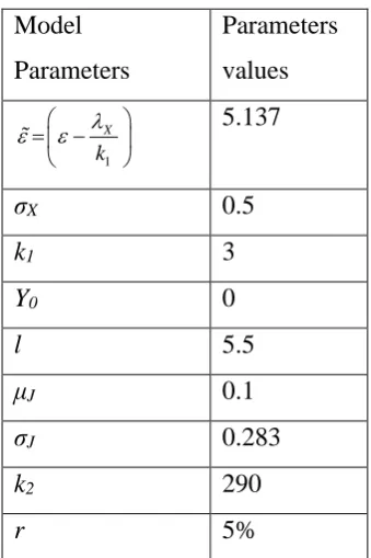
Figure 1: Implied volatility of European Call Options across different equilibrium levels
The figure shows the implied volatilities for European Call Options across varying levels of moneyness. We
consider three different equilibrium levels corresponding to cases when the risk neutral equilibrium level is equal
to the current spot price, exp
= P , (Base case), when it is below the current spot price (Low case) and when
it is above the current spot price(High case).
30% 50% 70% 90% 110% 130% 150% 170% 190% 210% 230%
75% 80% 85% 90% 95% 100% 105% 110% 115% 120% 125%
Moneyness in % (K/P)
Im
pl
ie
d
V
ol
a
ti
li
lt
y
Base Low Equilibrium High Equilibrium
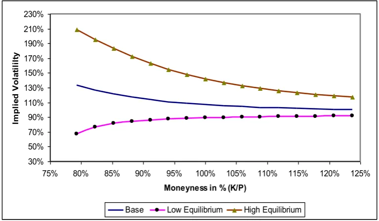
[image:15.595.105.489.469.693.2]we are moving from ITM to OTM call options and from OTM to ITM put options. Starting with the call options, we can note that the model displays some degree of skewness reflecting the fact that, due to mean reversion, prices do not fluctuate freely but are pulled back toward their mean. In the base and high cases, where the risk-neutral mean is equal and above the current spot price respectively, mean reversion is good for ITM call options since it pulls prices above the strike price and thus increases the likelihood that the options will end ITM; same is also true for the OTM options, however, since these options have lower probability of ending ITM, the impact of mean reversion is less beneficial compared to ITM options. Overall, this results in the skew evidenced in Figure 1. Turning next to the case where the equilibrium level is below the current spot price (i.e. the low case), we can see that volatility increases as strike price increases. This suggests that prices are now pulled toward lower levels due to mean reversion, and thus ITM calls are cheaper compared to calls calculated using the BSM model. OTM options on the other hand, are less affected by this since they have already a low probability of ending ITM, as the previous results showed. A similar pattern is observed in the case of put options, which are shown in Figure 2, where the implied model volatilities display exactly the opposite pattern from that of call options 5.
5 The general relationship between the shape of model implied volatilities for call and put options is similar to
Figure 2: Implied volatility of European Put Options across different equilibrium levels
The figure shows the implied volatilities for European Put Options across varying levels of moneyness. We
consider three different equilibrium levels corresponding to cases when the risk neutral equilibrium level is equal
to the current spot price, exp
= P , (Base case), when it is below the current spot price (Low case) and when
it is above the current spot price(High case).
30% 40% 50% 60% 70% 80% 90% 100% 110% 120%
75% 80% 85% 90% 95% 100% 105% 110% 115% 120% 125%
Moneyness in % (K/P)
Im
p
li
e
d
Vo
la
ti
li
ty
Base Low Equilibrium Hgih Equilibrium
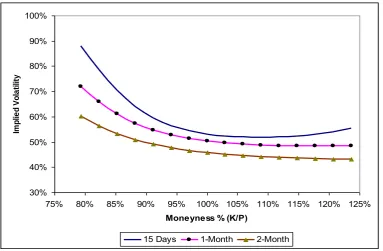
[image:17.595.106.492.212.434.2]Volatility Smile, Time to Maturity and Mean Reversion
Figure 3 compares the impact of changes in time to maturity on the implied volatilities of the spike model. First thing to note is that as time to maturity increases, implied volatilities decrease which is consistent with the Samuelson Hypothesis and depends on the speed of mean reversion, k1. This occurs because the BSM model implies that the variance of the spot
Figure 3: Implied volatility skew of the spike model for 15-day, one and two-month European Call Options.
The figure shows the implied volatilities for European Call Options based on the Spike model using the base
case parameters across different strike prices (Moneyness) and maturities (15-days, one- and two-months).
30% 40% 50% 60% 70% 80% 90% 100%
75% 80% 85% 90% 95% 100% 105% 110% 115% 120% 125%
Moneyness % (K/P)
Im
p
lie
d
Vo
la
ti
lity
15 Days 1-Month 2-Month
Focusing now on the skewness and kurtosis, it is evident from Figure 3 that there is a pronounced smile for short-term options which then seems to flatten-out, particularly for OTM options, as time to maturity increases 6. This pattern is consistent with a jump diffusion model and can also be explained by looking at the skewness and kurtosis of the risk neutral distribution in equations (6) and (7). Both moments decrease with time to maturity and speed of mean reversion, and ultimately go to zero (3 for kurtosis) for long enough expiration dates. It seems therefore that the jump diffusion model proposed here produces a pronounced smile for short-term options, and this smile gradually flattens-out out as time-to-maturity increases. This seems to be generally the case with jump diffusion models and, as shown by Rebonato (2004), in order to still have a pronounced smile for long-dated options, it is more appropriate to use a stochastic volatility model as in Heston (1993).
Another important factor affecting the volatility skew is the speed of mean reversion of the diffusive risk, which varies from market to market depending on a number of factors including the power-generation mix of each market. For instance, Escribano et al (2002) show
that the degree of mean reversion in hydro-markets is lower than that evidenced in fossil-fuel based power markets, since hydro reservoirs play the role of indirect storage of electricity; as a result, there is some inter-temporal substitution for generating electricity which can dampen short-term variations in power prices, thus lowering the coefficient of mean reversion. In markets with no inter-temporal substitution, on the other hand, we should observe a higher degree of diffusive mean-reversion since generators cannot use inventories to smooth-out shocks, and the degree of mean reversion in electricity prices is mainly driven by the mean reversion in demand or in temperature. Along the same lines, Elliot et al. (2002) also show that there is a link between the number of generators and the degree of mean reversion; when fewer generators are running, and thus when prices are higher, the degree of mean reversion is higher, compared to when all the generators are running and thus there is spare capacity in the market.
As the speed of mean reversion of the diffusive risk, k1, increases, we expect a similar pattern
to that observed in Figure 3. In particular, the higher the value of k1, the faster the volatility
will converge to a constant value and thus the lower the implied volatility. Similarly, we expect a more pronounced smile the slower the speed of mean reversion (i.e. for lower values of k1) and the smile will gradually flatten-out as the speed of mean reversion increases.
Therefore, an increase in the speed of mean reversion will have a similar impact on implied volatilities as that of increasing the time-to-maturity of the option and vice-versa.
Volatility smile and mean Jump Size
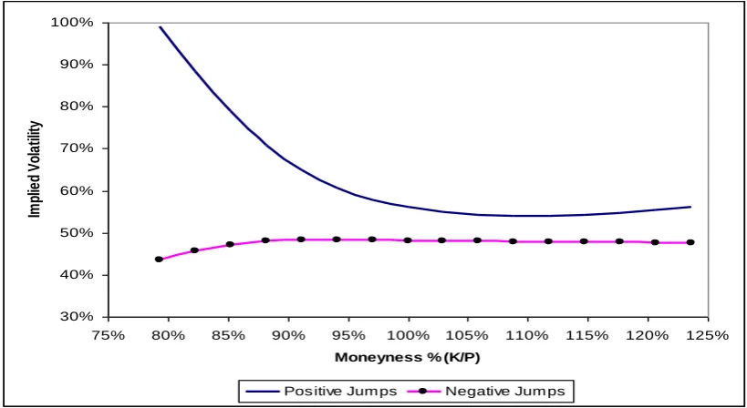
Figure 4: Implied volatility skew for 15-Day Call Options with respect to the sign of mean jump size μJ
The figure shows the implied volatilities for European Call Options with 15-days to maturity based on the spike
model across different strike prices (Moneyness), using positive and negative mean jump sizes, μJ, and the
remaining parameters being the same as in the base case, in Table 1.
30% 40% 50% 60% 70% 80% 90% 100%
75% 80% 85% 90% 95% 100% 105% 110% 115% 120% 125%
Moneyness % (K/P)
Im
pl
ie
d
Vo
la
til
ity
Pos itive Jum ps Negative Jum ps
As shown in equation (6), the sign of skewness depends on the sign of the expected jumps
( )l
E Jdq in log-returns, a fact that is depicted in Figure 4. If J is negative, the volatility
volatilities which decrease in an exponential fashion with strike prices, thus producing the negative skew shown in the graph. In the case of negative jumps, the probability mass is shifted to lower spot prices compared to the earlier case, which reduces the probability of call options to end ITM and results in lower implied volatilities. OTM options, on the other hand, are less affected by this since, due to mean reversion in prices, the probability of profitable exercise is already low.
Volatility smile curvature; Jump intensity versus Jump size volatility
Finally, we analyse the impact of jumpiness, which is the contribution of the jump component in the total variance as shown in equation (5). A jump diffusion model can be interpreted as a mixture of a pure jump process, as in the spike variable Y, and a diffusive process such as a GBM or a mean reversion. The issue is then to examine the impact of jumpiness on the smile and whether this is affected differently by changing each of the constituent components of jumpiness, namely σJand l. The two extreme cases are when the jumpiness is zero and the
[image:21.595.106.491.503.751.2]implied volatilities for OTM options become flat, and when the jumpiness is one in which case the smile has the maximum curvature.
Figure 5: Implied Volatility Skew for 15-Day European Call Options for different levels of jumpiness due to changes in Jump size volatility σJ
The figure shows the implied volatilities for European Call Options with 15-days to maturity for the Spike model
across different levels of moneyness, by changing the contribution of jumpiness to the total variance with respect
to σJ and all other parameters remaining the same as in the base case, in Table 1.
30% 40% 50% 60% 70% 80% 90% 100% 110%
75% 80% 85% 90% 95% 100% 105% 110% 115% 120% 125%
Moneyness % (K/P)
Im
pl
ie
d
V
ol
at
il
it
y
Figure 5 displays the implied model volatilities for different levels of jumpiness, expressed as the percentage of the total volatility given in equation (5), by changing the jump size volatility,J, for options that are 15-days to maturity. For instance, a 90% jumpiness level
means that jumpiness accounts for 90% of the total variance in equation (5) and this is achieved by changing the jump volatility, J , whilst keeping the jump intensity, l, the same as
[image:22.595.107.488.353.604.2]in the base case. We can see that that the smile becomes more pronounced as jumpiness increases and the implied volatilities of course are higher, since the overall volatility increases.
Figure 6: Implied Volatility Skew for 15-Day European Call Options for different levels of jumpiness due to changes in Jump intensity l
The figure shows the implied volatilities for European Call Options with 15-days maturity for the Spike model
across different levels of moneyness, by changing the contribution of jumpiness to the total variance with respect
to l and all other parameters remaining the same as in the base case, in Table 1.
30% 50% 70% 90% 110% 130% 150%
75% 80% 85% 90% 95% 100% 105% 110% 115% 120% 125%
Moneyness % (K/P)
Im
p
lie
d
Vo
la
ti
lity
10% 50% 75% 90%
the required percentage increase in intensity from the base case becomes very large; e.g. l
needs to increase by 800% from the base case in order to achieve 90% jumpiness, whereas the comparative increase for jump size volatility is 216%. It seems therefore that jump size volatility plays a more important role in affecting the jumpiness and thus the kurtosis of implied volatilities.
Table 2: Required percentage change in σJor l in order to achieve a given level of jumpiness
This table shows the required percentage change in jump size volatility, σJ, or jump intensity, l, compared to the base case (50% jumpiness), in order to reach a given level of jumpiness.
Jumpiness 10% 25% 50% 75% 90%
σJ -99.59% -50.00% 0% 80.28% 216%
l -88.89% -66.67% 0% 200% 800%
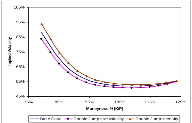
Another method for assessing whether it is the jump size volatility or intensity that contributes more to the smile curvature, is to employ the following three scenarios; one is the base case, using the same parameters as in Table 1, where jumpiness in equation (5) accounts for 50% of the total variance; in the second case, jump intensity is doubled in size and thus jump size volatility is lowered in order to keep the jumpiness at 50%, and in the third case, jump size volatility is doubled and jump intensity is lowered thus keeping again the jumpiness at 50%. The results are presented in Figure 7.
Of course we would also expect similar results for put options; in this case, the shape of the volatility smile is exactly the opposite from that of call, but the intuition remains the same.
Figure 7: Implied volatility Skew for 15-Day European Call Options with respect to Jump Intensity l and Jump Volatility σJ
The figure shows the implied volatilities generated from the spike model, when increasing by 100% either the
jump size volatility or the jump intensity, but always keeping the overall level of jumpiness at 50%.
45% 55% 65% 75% 85% 95% 105%
75% 85% 95% 105% 115% 125%
Moneyness % (K/P)
Im
p
lie
d
Vo
la
ti
lity
Base Case Double Jump size volatility Double Jump Intensity
5 Conclusions
that mean reversion reduces the volatility smile as time to maturity increases; interestingly, we find that even in the absence of jumps, mean reversion induces volatility skews particularly for ITM options. Finally, jump size volatility and jump intensity mainly affect the kurtosis and thus the curvature of the smile with the former having a more important role.
There are several implications based on these results. First, in a mean-reverting market, a participant using a GBM model will get misleading results; for instance, if the spot price is above the equilibrium price, a mean reverting model will price an ATM call closer to an OTM taking into account the fact that the price will have the tendency to revert to its equilibrium price, thus reducing the probability of ending ITM. On the other hand, the presence of jumps increases the probability of OTM options ending ITM, thus making exercise more likely; for instance, positive jumps will increase the values of OTM calls and negative jumps will increase the values of OTM puts. However, the overall impact of jumps on option prices will also depend on the spike-speed of mean reversion as well as the time-to-maturity of the option since the impact of jumps is higher for short-term options. Overall, an increase in the intensity and volatility of jumps will increase the price of OTM calls and puts, when compared to the Black-Scholes-Merton model.
6 REFERENCES
Bessembinder, H. and Lemmon, M.L., (2002), “Equilibrium Pricing and Optimal Hedging in Electricity Forward Markets”, Journal of Finance 57, 1347-82.
Black, F. (1976). The Pricing of Commodity Contracts. Journal of Financial Economics, vol (3), 167-169
Black, F. and Scholes, M. (1973), “The Pricing of Options and Corporate Liabilities”,
Journal of Political Economy, 673-54.
Branger, N., (2004), “An Option Pricing Anatomy”, Working Paper
Carr, P., and Madan, D., (2001), “Optimal Positioning in Derivatives Pricing”, Quantitative
Finance, 1, 19-37
Cerny, A., (2009), “Mathematical Techniques in Finance”, Princeton University Press,
Oxford, UK
Chacko, G. and Das, S., (2002), “Pricing Interest Rate Derivatives: A General Approach”,
Review of Financial Studies, 15(1), 195-241.
Clewlow, L., and Strickland, C., (2000), “Energy derivatives: Pricing and Risk
Dai, Q. and Singleton, K.J. (2000), “Specification analysis of affine term structure models”
Journal of Finance, Vol. 55, N° 5, 1943-1978.
Das, S.D., (2001),“The Surprise Element: Jumps in Interest Rates“, Journal of Econometrics, 106, 27-65.
Duffie, D., Pan, J. and Singleton, K. (2000) “Transform analysis and asset pricing for affine jump-diffusions”, Econometrica, vol. 68(6), 1343-1376.
Elliott, R.J., Sick, G. and Stein, M (2002), “Price Interactions of Baseload Supply Changes and Electricity Demand Shocks”, in Real Options and Energy Management, Ed. Ronn, E., Risk Books, London, 371-391.
Escribano, A., Peña, Juan. I. and Villaplana, P., (2002). “Modelling Electricity Prices: International Evidence,” Economics Working Papers, we022708, Universidad Carlos III, Departamento de Economía.
Ethier, S., and Kurtz, T., 1986, “Markov Processes, Characterization and Convergence”, New York: John Willey & Sons
Geman, H. and Roncoroni, A., 2006, “Understanding the Fine Structure of Electricity Prices”,
Journal of Business, Vol. 79, No. 3.
Geman, H., 2005, “Commodities and commodity derivatives: Modelling and Pricing for
Agriculturals, Metal and Energy” (Wiley Finance).
Glasserman, P., (2004), “Monte Carlo Methods in Financial Engineering”, Stochastic
Modelling and Applied Probability, Springer Finance.
Heston, S. (1993). “A Closed-Form Solution of Options with Stochastic Volatility with Applications to Bond and Currency Options”, Review of Financial Studies, 6, 327-343. Huisman, R., (2009), “An Introduction to Models for the Energy Markets”, Risk Publications,
London, UK.
Longstaff, F., and Wang, A., (2002), “Electricity Forward Prices: a high-frequency empirical analysis”, Working Paper, UCLA
Lucia, J. and E. Schwartz, (2002), “Electricity prices and power derivatives. Evidence from Nordic Power Exchange”, Review of Derivatives Research, vol. 5 (1), 5-50.
Merton R, (1973), “Theory of Rational Option Pricing,” Bell Journal of Economics and
Management Science 4:1, 141 – 183.
Merton R, (1976), “Option pricing when underlying stock returns are discontinuous,” Journal
of Financial Economics 3, 125-144.
Nomikos N, and Soldatos, O. (2008), “Using Affine Jump Diffusion Models for Modelling and Pricing Electricity Derivatives”, Applied Mathematical Finance, 15(1), p.41-71 Rebonato, R., (2004), “Volatility and Correlation: the Perfect Hedger and the Fox”, Wiley,
Samuleson, P. (1965) “Proof that properly anticipated prices fluctuate randomly”, Industrial
Management Review, 6, 13 - 31.
Schwartz, E. and Smith, J.E., (2000), “Short-term variations and long-term dynamics in commodity prices”, Management Science, 46 (7), 893-911.
Vasicek, O., 1977, “An Equilibrium Characterization of the term structure”, Journal of
Finance 5, 177-188.
Villaplana, P., (2003), “Pricing Power Derivatives: A Two Factor Jump-Diffusion approach, Working Paper, Universitat Pompeu Fabra.
7 Appendix A: Introduction and Application of the
Transform Function for the Forward Prices in the Factor
Model
A very useful assumption in the finance literature is that the state vector X follows an affine jump-diffusion process (AJD). An AJD is a jump-diffusion process for which the drift vector, the “instantaneous” covariance matrix, and jump intensities all have an affine (i.e. linear) dependence on the state vector. The affine jump-diffusion processes have been synthesized and extended by Duffie et al. (2000) (henceforth DPS); see also Chacko and Das (2002) and Dai and Singleton (2000). Affine diffusions (AD) and affine jump-diffusions (AJD) processes are quite useful in modelling underlying state variable due to their flexibility and tractability. DPS, for instance, have shown the close connection between the structure of affine models and Fourier transforms, and demonstrate how from this transform one can obtain derivative prices. The jump diffusion model presented in the main body of the paper belongs to the class of AJD. Hence, we can use the results provided by DPS in their transform analysis to obtain closed-form solutions implied by the spike model for forward and option prices.
The DPS transform can be described as follows: Fix a probability space {Ω, , P} and an information filtration (t) = {t:: t 0}, and suppose that Xt is a Markov process in some state spaceD n, following the stochastic differential equation (SDE):
d
X
t
(
X
t)
dt
(
X
t)
dW
t
dZ
t (9)Where Wt is an (t)-standard Brownian motion in n; (.) :D n, (.) : D n x n are respectively the drift and diffusion functions, and Zt is a pure jump process whose jump sizes
have a fixed probability distribution v on n
and arrive at frequency {l(Xt): t 0} for some l:
0,
has an infinitesimal generator of the Lèvy type, 7 defined at a bounded C2 function
f:D , with bounded first and second derivatives, by
1
( , ) ( , ) ( , ) ( ) ( , ) ( ) ( ) 2
( ) ( , ) ( , ) ( )
T t
f t f t f t tr f t
l f z t f t dv z
x xx
x x x x x x x
x x x (10)
Intuitively, (Xt)and (Xt) are the drift and diffusion terms of the process when no jump
occurs, and the jump term captures the discontinuous change of the path with both random arrival of jumps and random jump sizes. That is, conditional on the path of X, the jump times of the jump term are the jumps times of a Poisson process with, possibly, time-varying intensity {l(Xs): 0 s t}, and the size of the jump at a jump time m is independent of {Xs: 0 sm} and has the probability distribution v.
In order for the transform function to work, as stated by DPS (2000), the drift, variance-covariance, intensity and discount rate have to be affine functions of the state variables, hence:
0 1 0 1
0 1 ij 0 1
0 1 0 1
0 1 0 1
( ) , for ( , ) .
( ) ( ) , for ( , ) .
( ) , for ( , ) .
( ) , for ( , ) .
n n n
T n n n n n
ij ij
n
n
K K K K K
H H H H H
l l l l l l
R
x x
x x x
x x
x x
(11)
Let ( )
exp{ } ( )n
c c z dv z , be the characteristic function of the jump size distribution.
The function () determines completely the jump size distribution. Also assuming constant interest rates, R(x) = 0, futures prices are equal to forward prices. Let (K, H, l, ρ, θ)
which captures both the distribution of the vector process X as well as the effects of
7 The generator is defined by the property that
0
{ ( , ) ( , ) : 0}
t
t s
f X t
f X s ds t is a martingale for any fdiscounting, and determines a transform ψχ: n
D
of XT conditional on t,
when well defined at t T, by
( ,
, , )
exp
(
)
|
T
u T
t t s t
u
t T
E
R
ds e
X
X
X
(12)Where Eχ denotes the expectation operator under the distribution of Xdetermined by Hence the difference between the conditional characteristic function of XT and the transform function
ψχ is the discount factor R(XT). Therefore, under technical regularity conditions DPS (2000)
show that
( ) ( )
( , , , ) t t
t
u t T e
xX (13)
Where α and β satisfy the following complex-valued Ordinary-Differential-Equations:
1 1 1 1
0 0 0 0
1
( ) ( ) ( ) ( ) ( ) 1 ,
2 1
( ) ( ) ( ) ( ) ( ) 1
2 T T T T
t K t t H t l t
t K t t H t l t
(14)
With boundary conditions α(T)=0 and β(T)=u.
Application to the Spike Model
Now for the Spike model of equation (1) with constant jump parameters, the connection between the transform function and its use to find the forward prices is as follows:
1
2 2
*
( )
( ) exp
(
J,
J)
t t t
t X t X X
t t l
P
f t
X
Y
dX
k
X
dt
dW
dY
k Y dt
J
dq
(15) Therefore,
* * 1 2( ) exp ( , , , )
exp( ( ) ( ) ( ) )
r r r
t T t T T t
r
E P f T e E e X Y e u t T
e t t X t Y
X (16)
From (16) we use (14) to reach to the Ordinary Differential Equations and solve them:
1 2
1 2
and ( ) 1 ( )
Hence ( ) , ( )
k
i i
i i i i
k k
k T t e
t
t e t e
(17)
2 21 2 2
1
- 2 -2
2 2 - 2 -2
2
( ) 1
1 ( ( )) exp
2
1 1
( ) exp 1
2 2
k T s k T s
J J
T
k T s k T s k T s
k T s
X X J J
t
t e e
t r k e e l e e ds
Hence, using equation (16) and the results from equation (17), we have the expected value of the spot under the risk neutral probability measure:
1 2 2 2
0
- - - -2
* 2
0 0
0
( ) ( ) exp exp 1 1
2 t
t J J
t
k t k t k s k s
l A
E P f t e X Y e
e
e ds
1
11 2
-2
-1
1
22 1- (1- )
t
x k t x k t
A e e
k k
(18)
Using then equation (18) we define the de-seasonalised price of a forward contract for settlement at time T as follows:
* 0
(0, , ) ( T) ( )
F T X E P f t (19)
Proof of the formula for the security price G
a,b(y)
For0 < τ < ∞and a fixed y ,
( ) ( )
,
( ) ( )
,
, , 0, , , 0,
1 2 1 ( ; , , ) 2 1 ( ; , , ) 2 ivy ivy
iv z y iv y z
a b
iv z y iv y z
a b
e a ivb T e a ivb T
dv iv
e e
dG z T dv
iv
e e
dvdG z T
iv
X X X Xwhere Fubini is applicable because: lim a b,
; , ,
, , 0,
y G y T a T
X X given that χ is