Evolving Graphs: Dynamical Models, Inverse
Problems and Propagation
∗
Peter Grindrod
†Desmond J. Higham
‡August 28, 2009
Abstract
Applications such as neuroscience, telecommunication, on-line so-cial networking, transport and retail trading give rise to connectivity patterns that change over time. In this work we address the resulting need for network models and computational algorithms that deal with dynamic links. We introduce a new class of evolving range-dependent random graphs that gives a realistic but tractable framework for mod-eling and simulation. We develop a spectral algorithm for calibrating a set of edge ranges from a sequence of network snapshots, and give a proof of principle illustration on some neuroscience data. We also show how the model can be used computationally and analytically to investigate the scenario where an evolutionary process, such as an epidemic, takes place on an evolving network. This allows us to study the cumulative effect of two distinct types of dynamics.
Keywords: birth and death process, epidemiology, network, neuroscience, random graph, reproduction rate.
1
Introduction
The last decade has seen a huge rise in interest in complex networks and their applications to mass communication, social, and interaction phenom-ena. Until recently, one characteristic of such networks that is fundamental
∗This manuscript appears as University of Strathclyde Mathematics Research Report 26
(2009).
†Department of Mathematics and Centre for Advanced Computing and Emerging
Tech-nologies, University of Reading, RG6 6AX, UK
‡Department of Mathematics and Statistics, University of Strathclyde, Glasgow G1
within some applications has been rather neglected: that the networks may evolve [2, 7]. When new edges may appear and existing edges may disap-pear there is an important interaction between dynamics on the network and dynamics of the network. This topic is distinct from network growth, or aggregative phenomena: it embodies the property that all edges within the network are transient to some extent. Very recently, general classes of dynamic networks have been proposed and studied in the theoretical com-puter science literature [1, 3, 4] from a complexity theory perspective. Our work looks at complementary issues driven by the need for practical tools in modelling, calibration and data analysis.
In [2] it is pointed out that network evolution can be approached from distinct directions: at the macro level, it may be observed within real data sets by studying the time course of global parameters from one snap shot to another, or at the micro level, dynamic properties could be ascribed to the individual birth-death rules for each edge; and that specific applications will require some analytical methods to approach aninverse problem: given some data from a time dependent evolving network, how best may one represent it within a suitably defined class of models?
In this paper we consider these problems and offer an operational ap-proach to each.
In section 2 we consider micro-to-macro models which produce evolving networks, considered as classes of Markov processes defined over the set of all possible undirected graphs on a finite set of n vertices. This space grows asO(2n2
), so we suggest simplifying to the case of independent dynamics for each edge.
As a further simplification, we may then allow the dynamics to depend only on the range of the edge. This extends the static concepts of “lat-tices plus shortcuts” [13, 14, 18] and more general range dependent random graphs [9, 12] to the dynamic setting. In many applications, vertices are fixed within some Euclidean or underlying metric space and each edge has a natural “range” representing the distance between the end vertices, which may impact on the possibility of that edge arising. For example in traditional acquaintanceship networks physical neighbors have a good chance of knowing each other. These ideas are pervasive in the literature; see, for example, the recent treatment in [6]. But in many applications, there is no obvious, fixed lattice topology. For example
• in communication networks, individuals may be mobile,
• in cyberspace, hyperlinks are not constrained by the underlying internet connectivity structure,
• in high frequency functional connectivity networks from neuroscience, cognitive processing tasks may be distributed across the brain,
• in proteomic interaction networks, connections may be caused by a combination of features, including electrostatic, hydrophobic or chem-ical similarities rather than any obvious sequence-level or geographchem-ical commonalities.
In all these cases the concept of “range” is more elusive, but can still have some meaning. The range of an edge reflects the transitive nature of the connection. If vertex a is connected to vertex b which is in turn connected to vertex c, how likely is it that vertex a is also connected to vertex c? If it is very likely then we will say that connection is (locally) transitive and the edge from a to cis short range, if it is very unlikely then the edge from
a to c is long range. Cliques are full of short range edges. Hence when we are presented with data from an evolving graph as just a transient set of connections between an arbitrarily ordered list of vertices, there is potential to add insight by inferring a range for every possible edge. This is theinverse problem we will address: that of representing a given evolving graph as a range dependent evolving graph and thus inferring a range for every possible edge.
2
Independent edge-dependent dynamics
Let Vn denote a set of n labelled vertices. Let Sn denote the space of all
undirected graphs defined on Vn. Then |Sn|= 2n(n−1)/2. Any element of Sn,
denoted by a, may be represented by ann×n symmetric adjacency matrix, which we will denote by A.
We will consider discrete time Markov processes defined over Sn, whose
paths consist of time dependent sequences of elements, {aj} in Sn, each
representing the evolving graph at time tj = j δt. Even when we restrict to
the case where the transition matrix is time-independent, to fully specify such a process, in general, requires 2n(n−1) non negative graph-to-graph transition
probabilities. We therefore continue with a simplified class of models where the time dependent appearance or disappearance of each individual edge is governed by a random process that is independent of all other edges. More precisely, consider an evolving graph{aj}defined as follows. Letα(e) denote
the probability that any edge, e, not part of the network at time t may be added to it over the time step δt. Let ω(e) denote the probability that any edge, e, that is part of the network at time t will be removed over the time step δt. So α and ω specify the birth and death probabilities, respectively, that we assume to be O(δt) forδt small.
For any paira, a′
∈Sn, let P(a′|a) denote the probability thataj+1 =a′
given that aj = a, and let E(a) denote the set of edges belonging to a.
Then the “independent edge-dependent” model yields the graph-to-graph transition probability
P(a′
|a) = Y
e∈E(a′), e /∈E(a)
α(e) Y
e /∈E(a′), e /∈E(a)
(1−α(e))×
Y
e /∈E(a′), e∈E(a)
ω(e) Y
e∈E(a′), e∈E(a)
(1−ω(e)). (1)
This expression gives the probability that exactly the right subsets of edges are added and deleted to achieve the required transition. As a result of the edge independence assumption, there are now n(n−1) parameters (the
α(e) andω(e)) rather than the 2n(n−1) required in the general case.
It is straightforward to calibrate such a model, given sufficient data. Sup-pose that we observe a sequence {ˆaj|j = 1, ..., J}. Then we may estimate the
e (so e appears in those transitions). Then we have the following estimate
b
α(e) = m(e) + 1
M(e) + 2. (2)
Similarly suppose an edge e occurs within the first J −1 terms of the ob-served sequence of graphs on exactly M⋆(e) occasions, and of these graphs
exactly m⋆(e) are followed by graphs that do not contain e (so e is lost in
the transition). Then
b
ω(e) = m
⋆(e) + 1
M⋆(e) + 2. (3)
We may then use these estimates in (1) to generate any graph to graph transition probability that is required. In particular we could simulate and analyze sequences of networks.
3
Range Dependent Random Graphs
In [9] the class of range dependent random graphs was introduced as a pa-rameterized model that can reproduce important properties seen in real net-works. Protein-protein interaction data was used to motivate and justify the concept. Closely related models based on similar principles include
• the original small world networks of Watts and Strogatz [23], and their counterparts based on adding shortcuts rather than rewiring [18], where edges are either long or short range,
• the two-dimensional lattice based model of Kleinberg [14, 15],
• the geometric model used by Pruzlj and co-workers [16, 19] to describe protein-protein interactions.
Range dependent random graphs are best introduced by imagining the ver-tices set out in a line and labeled by their integer positions. To simplify things further, ifn, the number of vertices, approaches infinity, then we may approx-imate the graph by one on infinitely many vertices (. . . ,−2,−1,0,1,2, . . .), since the edge effects become less important.
Range dependent random graphs are then defined as follows: an edge is present between any vertices i1 and i2 with probability pi1,i2 = f(|i1 −i2|), where f is a given monotonically decreasing function of the edge range |i1−
i2|. Thus, in this model the presence or absence of an edge depends only
on its range, and each edge is independent. Letting Pk be the consequent
P∞
k=1xkPk can be used to study the Watts-Strogatz clustering coefficient
[23], and the mean degree; see [9] for details.
In the protein-protein interaction case, and in most realistic network sce-narios, the vertices will be labelled in a way that does not reflect any edge range information. So there is a natural inverse problem of reordering the vertices to reveal the range dependency. Genetic algorithms [9] and more efficient spectral methods [10, 11] have proved successful in this context.
Our aim is now to develop these static ideas into the evolving graph framework.
4
Evolving Range Dependent Random Graphs
Consider a set of n vertices labelled by locationi = 1, ..., n. As in section 2 we consider a discrete Markov process over Sn where all edges evolve
inde-pendently. Suppose further that each edgeehas transition probabilities that depend only on its range: if an edge connects vertices i1 and i2, then we will
write k(e) =|i1−i2|to denote its range. Then an evolving range dependent
random graph has birth and death transition probabilities
α(e) = fα(k(e)), ω(e) = fω(k(e)),
given by functionsfα(k) and fω(k) that map the positive integers onto [0,1].
Now let p(e, j) denote the probability that the edge e is present within
aj, the graph at time tj. Then using the transition probabilities above we
have the dynamical equation
p(e, j+ 1) =fα(k(e))(1−p(e, j)) + (1−fω(k(e))p(e, j).
A steady distribution must then satisfy
p0(k(e)) =
α(e)
α(e) +ω(e) =
fα(k(e))
fα(k(e)) +fω(k(e))
, (4)
which depends only upon k(e). Hence, at equilibrium any single observation of the evolving graph appears as a range dependent random graph with each edge present according to this range dependent probability function p0(k).
Now consider the natural inverse problem. Given an observed sequence, {ˆaj|j = 1, ..., J}, with the vertices in some given orderingi= 1, ..., n, how can
The simplest way forward is to consider each edge in turn within the evolving sequence. Suppose that e = (i1, i2), in the original ordering, is
observed on exactly ri1,i2 occasions (and is absent on J −ri1,i2 occasions). LetRdenote the symmetric nonnegative matrix with elementsri1,i2. Under a reorderingq(i) the edge range becomesk(e) = |q(i1)−q(i2)|and the likelihood
of the observations for this edge is given by
p0(|q(i1)−q(i2)|)ri1,i2.(1−p0(|q(i1)−q(i2)|))J−ri1,i2.
Trivially we can rewrite this as
p0(|q(i1)−q(i2)|)ri1,i2
(1−p0(|q(i1)−q(i2)|))ri1,i2(1−p0(|q(i1)−q(i2)|))
J.
Since all edges are independent we may write the likelihood over the entire graph by taking a product over all possible edges, to give
Y
e=(i1,i2)
p0(|q(i1)−q(i2)|)ri1,i2 (1−p0(|q(i1)−q(i2)|))ri1,i2
Y
e=(i1,i2)
(1−p0(|q(i1)−q(i2)|))J.
But the second product is independent of q since all possible edges appear and are raised to the same power. Thus the likelihood of these observations, given any q, has the proportionality
L(q)∝L(bq) := Y
e=(i1,i2)
p0(|q(i1)−q(i2)|)
(1−p0(|q(i1)−q(i2)|)) ri1,i2
.
So we should chose a reordering q to maximize L(q). From (4) we thus have
b
L(q) = Y
e=(i1,i2)
fα(|q(i1)−q(i2)|)
fω(|q(i1)−q(i2)|) ri1,i2
. (5)
MaximizingLbin (5) over all reorderingsqis a hard combinatoric optimization problem. We can make progress through two types of simplification.
First, we assume that the ratio of birth and death transition probabilities has the functional form
fα(k)
fω(k)
∝θk2, (6)
for some constant θ. Then taking logarithms in (5) we have
logL ∝b log (θ)X
i1>i2
ri1,i2(q(i1)−q(i2))
The second step is to relax the problem so that q is allowed to be a real-valued vector. The right-hand side in (7) may be written as the quadratic formqT∆
Rq. Here ∆R, the Laplacian matrix associated withR, has the form
D−R, where the diagonal matrix D contains the row/column sums of R. To remove shifting and scaling redundancies we also impose the constraints kqk2 = 1 andPni=1q(i) = 0.
We now have a tractable optimization problem. For applications where the death rate exceeds the birth rate at long range, so θ < 1, it is solved by a Fielder vector—an eigenvector corresponding to the smallest nonzero eigenvalue of ∆R. A reordering of the vertices can be recovered by sorting
the components ofq; that is, vertexiis placed before vertexj ifqi < qj. This
approach has been found to be effective for static networks [5, 8, 10, 11, 12, 20, 22]; here we are showing that in the evolving case it is possible to justify from first principles the idea of reordering on the cumulative (non-binary) matrix R.
We point out that it is not necessary to know the actual value of θ in (6). The derivation assumes only that this functional form exists and θ is not required by the algorithm. We have found in practice that performance is not sensitive to the precise form of range-dependency [11], especially in the long range, or large k, regime. Furthermore, this approach of spectral reordering based on R can be used for any data set, and the validity of (6) may then be tested a posteriori.
We also note that the reordering approach continues to make sense when
θ > 1 in (6). This includes the case where long ranges are very unlikely to emerge, but those that do are long-lived. In this case, because log (θ) > 0, the expression in (7) is maximized by an eigenvector of the Laplacian that corresponds to a dominant eigenvalue.
5
Computational Results for Reordering an
Evolving Graph
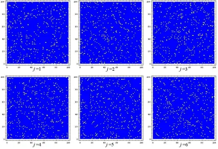
To test the reordering approach, we generated some synthetic data from the appropriate underlying model. With n= 100 vertices, we chose a birth rate
fα(k) = 0.1(0.98)k
2
and death rate fω(k) = 0.2. Figure 1 shows the first
six adjacency matrices. Here, nonzeros in the adjacency matrix are marked with light dots. We have used an arbitrary vertex ordering, so the range dependent nature of the networks is not apparent.
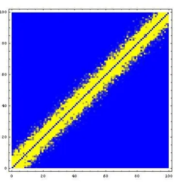
Figure 2: The reordered sum (superposition) of the evolving graph after maximizing the relaxed likelihood.
all 200 timesteps; a light dots denotes that an edge was present for at least one time step. Figure 3 shows a typical member of the sequence in this new ordering. We see from Figures 2 and 3 that the hidden range dependency has been revealed by the algorithm.
Next, we illustrate the algorithm in an electroencephalography (EEG) application, using data from [21]. Here, the measurements represent electrical activity produced by the firing of neurons within the brain over a short period of time, reflecting correlated synaptic activity caused by post-synaptic potentials of nearby cortical neurons.
In these experiments, the subject carried out a specific task—tapping in time to music. We use four seconds worth of data sampled at 500Hz, with two seconds prior to tap and two seconds after. Hence the finger tap starts around 1000 samples into the data. Measurements were taken at each of 128 electrodes arranged at fixed points on the scalp.
Figure 3: A typical reordered element of the evolving network.
be distributed across the cortex.
We therefore let each electrode represent a vertex within an evolving graph. We subdivided the time dependent data into windows of 50 consec-utive time steps, each lasting 0.08 seconds. Within each time step we first obtained the all vesus all channel correlation matrix, and defined an edge between vertex i and vertex j if this correlation exceeded 0.8. This resulted in an evolving sequence of 50 adjacency matrices.
We note that correlation between signals is a far from perfect measure, especially in the search for noisy, transient, synchronous components within time series: but it will serve for our current purpose of illustrating how naturally the concept and methods of evolving (organizational) graphs, in-troduced in this paper, may represent the coordinated emergent, transient, responses (both local and non local) of the brain.
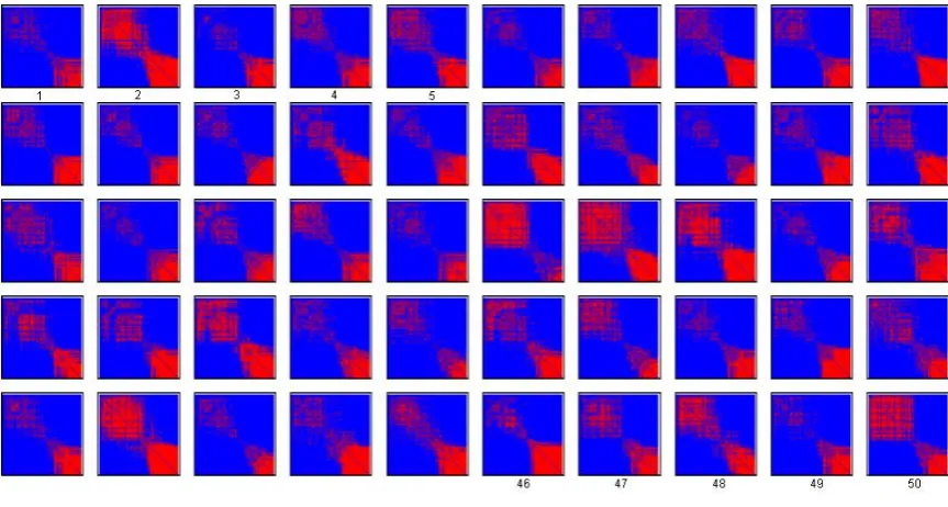
Figure 4: An evolving sequence of 50 adjacency matrices that represent cor-relations between brain activity at 128 regions. Vertices are ordered using the default provided by the recording equipment.
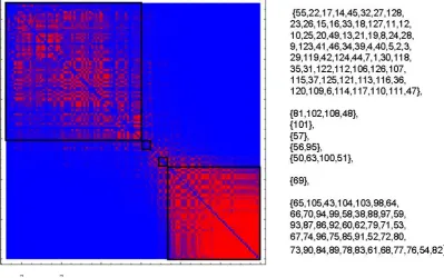
geographically close to the latest. This effect manifests itself through the sig-nificant nonzero blocks in the off-diagonal corners of the adjacency matrices. Figure 5 repeats the information in Figure 4, with vertices reordered via the spectral algorithm. In this case we see that the activity has been arranged into coherent blocks. At the latter end of this new ordering (lower right corner), one set of vertices appears to have a consistently strong set of mutual correlations, whereas at the start (upper left corner) a more transient set of correlations is captured. The apparent periodicity from Figure 4 has been removed and there is a clear propensity for ‘short range’ edges; that is, connections between near-neighbours.
Figure 5: The adjacency matrices from Figure 4, reordered according to the range dependency algorithm.
As ana posteriori check on the relevance of the evolving network model, in Figure 7 we scatter plot the values
1
k2 log
b
α(k)
b
ω(k)
,
whereαb(k) andωb(k) are computed from (2) and (3). If the assumption (6) is valid, then these values provide estimates for logθ. For each predicted range,
k, the solid line in the figure shows the average of the scattered points, and we see that the results are consistent with the θ < 1 scenario to which the algorithm applies.
Figure 7: Scatter plot (gray) and average (dark line) of the scaled log birth data ratio (log(αb(k)/ωb(k))/k2 as a function of predicted range, k.
6
Simulating propagation within an evolving
graph
To put dynamics on the evolving network, suppose we have a binary state variable defined at each vertex and at each timestep. To be specific, let this variable take values “infected” and “susceptible”. Initially all vertices except one are labeled susceptible.
From one time step to the next, we impose the following simple dynamics, depending on a single parameter µ.
• A susceptible vertex has no effect on the fate of any other vertex.
• Each infected vertex passes on the infection to all of its current imme-diate neighbors.
• Having passed on the infection, each infected vertex becomes suscep-tible with probability 1−µ, or else remains infected, with probability
µ.
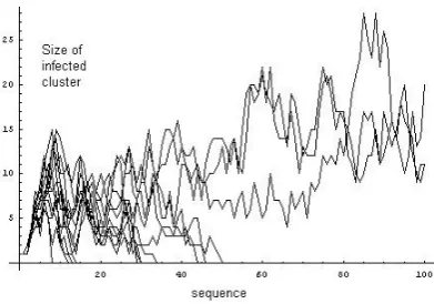
Figure 8: Propagation of infection through the evolving graph as recovery rate lessens.
at individual vertices for a long time and these vertices eventually acquire edges), but not for small µ; or the evolving network is dense enough to sup-port spreading for all values of µ—even when µ= 0 so the infection lasts for just one timestep at each infected vertex. In the special case where µ = 1 and every α is positive, we are in thesuccessive percolation or flooding [3, 4] regime where all vertices are certain to become infected,
The novelty in this area lies in the dynamic coupling between the evolu-tion of the contact network and the time course of the infecevolu-tion, in contrast with most of the existing work in this field, which has been carried out with percolation type models or SIR dynamics on static graphs.
In Figure 8, we depict a threshold case, where the elements of the evolving (range dependent) network are individually very sparse; the expected degree is 0.79. All elements are highly disconnected. In this example we use the same evolving network in each case with 100 vertices, for which fα(k) = 0.1(0.9)k
2
and fω(k) = 0.5. We seed the infection at a single vertex (vertex 40), with a
different value ofµfor each run. We emphasize that recovery at each infected vertex is decided independently at random in all cases (a Poisson process). We employ values forµbetween 0.1 (where the infection dies out quickly) up to .625, where it propagates over the whole evolution. The threshold observed to be approximately between .55 and .575. So we have an example of how occasional long range transient connections between otherwise short range, isolated communities, may propagate disease providing that the infectious period for individuals (and hence of the isolated communities) is long term enough.
Figure 9: Mean and mode of the shortest transmission time versus message range; and density plot for shortest transmission time versus message range, obtained from 17300 experiments.
at each time step the message is relayed to any vertices directly connected to previous message holders. Hence the message spreads according to the successive edges added at each time step to the existing message holders. Eventually all vertices will receive the message (since µ= 1 so a vertex never forgets the message). Suppose also that a vertex is designated as the desired
receiver. Then, in the range dependent graph setting, there is a natural range between sender and receiver, which we will denote by kmess. We will say the
the minimum number of time steps needed for the first arrival of the message at the receiver is theshortest transmission time(STT). It is clearly of interest to study the distribution of the STT and related quantities, such as the natural ‘path length’ measured by taking whichever message-holding vertex is currently closest in range to the receiver. This path length is important if, for example, the message propagation from one vertex to another along any single edge during any single time step is noisy, so that a “Chinese Whisper” effect accentuates such noise.
Forfα(k) = 0.1(0.9)k
2
and fω(k) = 0.5 we have an average degree at any
7
Analysing propagation within an evolving
graph
We now show that the evolving random network model used in Figures 8 and 9 is sufficiently compact to allow for some theoretical analysis.
In order to understand the behaviour seen in Figure 9, we will make two simplifying assumptions.
1. At each time step, the nearest vertex to the receiver, say A, either remains the nearest vertex, or the new nearest vertex arises from an edge that has appeared from vertexA. We may then assume that each new edge utilized is independent of the previous ones (since we make no assumption about any edge leaving A, prior to the arrival of the message at A).
2. The “edge effects” caused by the requirement that the message exactly reaches the receiver can be ignored, so that we can focus on the general phase where the message progresses as quickly as possible away from the sender.
In any element of the evolving graph, we have the equilibrium probability that any edge of length k is present at a particular time step given by (4).
Consider any particular vertex that the message has reached, and letπ(k) denote the probability that the longest range of any edge connected to it is exactly equal to k. Then we have directly
π(0) =
∞
Y
j=1
(1−p0(j))2,
π(k) = (2p0(k)−p0(k)2)
∞
Y
j=1
(1−p0(k+j))2, k≥1.
The sequence {π(k)} sums to one, and we can use these forms to calculate the expected range of the longest range edge connected to any vertex (=
P
kπ(k)).
Similarly, let π⋆(k) denote the probability that the longest range of any
edge connected the particular vertexin the direction of the receiver is exactly equal to k. Then we have
π⋆(0) =
∞
Y
j=1
(1−p0(j)),
π⋆(k) = p0(k)
∞
Y
The expected range of the longest range edge in the direction of the receiver is thus Pkπ⋆(k).
For the choices of fα(k) andfω(k) in Figure 9, the expected range of the
longest range edge is given by 1.3598 in any direction. Similarly the expected range of the longest range edge in the direction of the receiver is given by LRE=0.773.
Under our simplifying assumption that edges transmit the message in the direction of the receiver, we have
STT = kmess/LRE= 1.293 kmess.
This explains the slope of the mean and mode curves in Figure 9. Over long message ranges we may appeal to the central limit theorem: the message propagates according to a process that could be subdivided into independent increments, for much shorter message ranges, successively drawn from a dis-tribution of paths for the shorter ranges. Thus the message arrival behaviour and time resembles that for a diffusion-advection process.
Of those successive time steps we expect that a fraction π⋆(0) = 0.657
made no progress towards the receiver—the range of the longest edge in the receiver’s direction being zero, for that time step at the closest vertex.
Hence the message travels a total message range of kmess, over 1.293
kmess successive time steps, along approximately 1.293(1 − 0.657)kmess =
0.442kmess edges. Notice that the expected range of the longest range edge in
the direction of the receiver, given that it is not zero, is simplyPkπ⋆(k)/(1−
π∗(0)), which is approximately 2.25.
For the computations shown in Figure 8, we observed a threshold value for µ governing overall growth or decay of the disease. To understand this behaviour and estimate the critical µ, we consider, at equilibrium, a single infected vertex, A. Our aim is to estimate the number of new vertices that
A infects before its eventual recovery. The expected degree of nodeA on the next step is the sum over the probability of all possible edges,
b
d:= 2
∞
X
k=1
p0(k), (8)
where p0(k) is defined in (4). Some of the vertices that A points to may
already be infected, of course. In particular, the most likely already-infected neighbour is the vertex, sayB, that infectedA. Because the edge death rate,
fω, is constant in this experiment, this value gives the probability that the
edge connecting B to A remains over one step. So the probability that the edge A-B remainsand vertexB has not recovered is fωµ. Hence, correcting
b
d in (8) to discount “infection” of an already infected node B, we arrive at
˜
as our approximation to the expected number of new infections caused by A
after one step.
Now let us consider new edges appearing at subsequent steps. Suppose we consider any such edge, of length k. This edge is not present on the first time step post-infection with probability 1 −p0(k). The probability that
it first appears as a new edge on exactly the jth time step post-infection (j = 2,3, . . . .) is thus
(1−p0(k)) (1−fα(k))j
−2 fα(k).
(This expression arises as the product of the probabilities that the edge (a) is missing on the first step, (b) does not appear in steps 2 through to j−1 and (c) appears at step j.) The expected number of edges connecting to vertex
A for the first time at the jth time step post-infection is thus
2
∞
X
k=1
(1−p0(k)) (1−fα(k))j
−2
fα(k).
The probability that vertexA is still infectious at the jth step following infection is µj−1. So, summing over all times, our overall approximation of
the expected number of new vertices that A infects before recovery is
R(µ) := ˜d+ 2
∞
X
j=2
µj−1
∞
X
k=1
(1−p0(k)) (1−fα(k))j
−2
fα(k). (9)
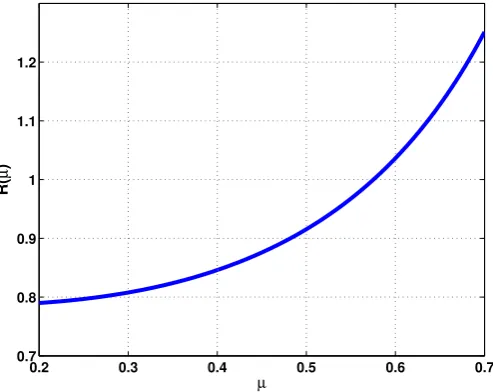
This quantity is analogous to the basic reproduction rate, usually called R0,
that arises in classical epidemiology [17], and we are therefore interested in the critical value R(µ) = 1.
For the case fω = 0.5, fα(k) = 0.1(0.9)k
2
used in Figure 8, we show in Figure 10 the behaviour of R(µ) in (9). Solving numerically, we find that
R(µ) = 1 atµ= 0.575, which matches well with the experimentally observed threshold.
8
Discussion
0.2 0.3 0.4 0.5 0.6 0.7 0.7
0.8 0.9 1 1.1 1.2
µ
R(
µ
[image:21.595.171.418.310.506.2])
development. We showed that the evolving network model adds value to some real brain activity data, but we believe that, due to the generic nature of the modelling assumptions, the same approach will be applicable to many other scenarios where sparse network “snaphots” are observed, including ap-plications in telecommunications, sociology and business.
Although our evolving network model was set up as a discrete time Markov chain, we remark that an analogous continuous time framework could developed, which might be more suited to rigorous probabilistic analysis.
The evolving network model can also be combined with a time dependent process that acts over the network. We showed via simulation and analysis that the overall behaviour of the resulting stochastic process depends strongly on the interaction between the two sets of dynamics. There is much scope here for adding realistic topological dynamics to the traditional static network models of disease propagation and message passing.
Acknowledgements We thank Slawomir Nasuto for making available some data from [21] and for helpful discussions about the computational results.
The authors acknowledge support from EPSRC through project grant GR/S62383/01 and Bridging the Gaps ‘Cognitive System Science’ grant EP/F033036/1.
References
[1] C. Avin, M. Kouck´y, and Z. Lotker, How to explore a
fast-changing world (cover time of a simple random walk on evolving graphs), in ICALP ’08: Proceedings of the 35th international colloquium on Au-tomata, Languages and Programming, Part I, Berlin, Heidelberg, 2008, Springer-Verlag, pp. 121–132.
[2] P. Brognat, J.-L. Guillaume, C. Magnien, C. Robardet, and
A. Scherrer, Evolving networks, preprint.
[3] A. E. Clementi, C. Macci, A. Monti, F. Pasquale, and R.
Sil-vestri, Flooding time in edge-Markovian dynamic graphs, in
Proceed-ings of the 27th Annual ACM SIGACT-SIGOPS Symposium on Princi-ples of Distributed Computing (PODC’08), ACM Press, 2008, pp. 213– 222.
[4] A. E. Clementi, A. Monti, F. Pasquale, and R. Silvestri,
[5] C. H. Q. Ding, X. He, H. Zha, M. Gu, and H. D. Simon, A min-max cut algorithm for graph partitioning and data clustering, in Proceedings of the 1st IEEE Conference on Data Mining, 2001, pp. 107– 114.
[6] M. Franceschetti and R. Meester, Random Networks for
Com-munication: From Statistical Physics to Information Systems, Cam-bridge Series in Statistical and Probabilistic Mathematics, 2008.
[7] A. Gautreau, A. Barrat, and M. Barthelemy,
Microdynam-ics in stationary complex networks, Proc. Nat. Acad. Sci., 106 (2009), pp. 8847–8852.
[8] A. George and A. Pothen, An analysis of spectral
envelope-reduction via quadratic assignment problems, SIAM Journal of Matrix Analysis and its Applications, 18 (1997), pp. 706–732.
[9] P. Grindrod, Range-dependent random graphs and their application
to modeling large small-world proteome datasets, Physical Review E, 66 (2002), pp. 066702–1 to 7.
[10] P. Grindrod, D. J. Higham, and G. Kalna, Periodic reordering,
Institute Maths Appls J. Numerical Analysis, (submitted).
[11] D. J. Higham, Unravelling small world networks, J. Comp. Appl.
Math., 158 (2003), pp. 61–74.
[12] , Spectral reordering of a range-dependent weighted random graph, IMA J. Numer. Anal., 25 (2005), pp. 443–457.
[13] , A small world phenomenon for Markov chains, SIAM Review, 49 (2007), pp. 91–108.
[14] J. Kleinberg,Navigation in a small world, Nature, 406 (2000), p. 845.
[15] , The small-world phenomenon: An algorithmic perspective, Proc. 32nd ACM Symposium on Theory of Computing, (2000).
[16] O. Kuchaiev, M. Raˇsajski, D. J. Higham, and N. Prˇzulj,
Ge-ometric de-noising of protein-protein interaction networks, PLoS Com-putational Biology, (To appear).
[17] J. D. Murray, Mathematical Biology: I. An Introduction, Springer,
[18] M. E. J. Newman, C. Moore, and D. J. Watts, Mean-field so-lution of the small-world network model, Physical Review Letters, 84 (2000), pp. 3201–3204.
[19] N. Prˇzulj, D. G. Corneil, and I. Jurisica,Modeling interactome:
scale-free or geometric?, Bioinformatics, 20 (2004), pp. 3508–3515.
[20] G. Strang, Computational Science and Engineering,
Wellesley-Cambridge Press, 2008.
[21] C. M. Sweeney-Reed and S. J. Nasuto, Detection of neural
cor-relates of self-paced motor activity using empirical mode decomposition phase locking analysis, Journal of Neuroscience Methods, (to appear, 2009).
[22] R. Van Driessche and D. Roose, An improved spectral bisection
algorithm and its application to dynamic load balancing, Parallel Com-puting, 21 (1995), pp. 29–48.
[23] D. J. Watts and S. H. Strogatz, Collective dynamics of