Displaced Solar Sail Orbits: Dynamics and
Applications
Jules Simo
∗and Colin R. McInnes
†University of Strathclyde, Glasgow, G1 1XJ, United Kingdom
We consider displaced periodic orbits at linear order in the circular restricted Earth-Moon system, where the third massless body is a solar sail. These highly non-Keplerian orbits are achieved using an extremely small sail acceleration. Prior results have been de-veloped by using an optimal choice of the sail pitch angle, which maximizes the out-of-plane displacement. In this paper we will use solar sail propulsion to provide station-keeping at periodic orbits around the libration points using small variations in the sail’s orientation. By introducing a first-order approximation, periodic orbits are derived analytically at linear order. These approximate analytical solutions are utilized in a numerical search to deter-mine displaced periodic orbits in the full nonlinear model. Applications include continuous line-of-sight communications with the lunar poles.
I.
Introduction
O
ver several years, solar sailing has been studied as a novel propulsion system for space missions. Solar sail technology appears as a promising form of advanced spacecraft propulsion which can enable exciting new space-science mission concepts such as solar system exploration and deep space observation. Although solar sailing has been considered as a practical means of spacecraft propulsion only relatively recently, the fundamental ideas are by no means new (see McInnes1 for a detailed description). A solar sail is propelledby reflecting solar photons and therefore can transform the momentum of the photons into a propulsive force. Solar sails can also be utilised for highly non-Keplerian orbits, such as orbits displaced high above the ecliptic plane (see Waters and McInnes2). Solar sails are especially suited for such non-Keplerian orbits, since
they can apply a propulsive force continuously. In such trajectories, a sail can be used as a communication satellite for high latitudes. For example, the orbital plane of the sail can be displaced above the orbital plane of the Earth, so that the sail can stay fixed above the Earth at some distance, if the orbital periods are equal (see Forward3). Orbits around the collinear points of the Earth-Moon system are also of great
interest because their unique positions are advantageous for several important applications in space mission design (see e.g. Szebehely4, Roy,5 Vonbun,6 G´omez et al.7,8). In recent years several authors have tried
to determine more accurate approximations (quasi-Halo orbits) of such equilibrium orbits9. These orbits
were first studied by Farquhar10, Farquhar and Kamel9, Breakwell and Brown11, Richardson12, Howell13,14.
If an orbit maintains visibility from Earth, a spacecraft on it (near the L2 point) can be used to provide
communications between the equatorial regions of the Earth and the lunar poles. The establishment of a bridge for radio communications is crucial for forthcoming space missions, which plan to use the lunar poles. McInnes15 investigated a new family of displaced solar sail orbits near the Earth-Moon libration points.
Displaced orbits have more recently been developed by Ozimek et al.16using collocation methods. In Baoyin
and McInnes17,18,19 and McInnes15,20, the authors describe new orbits which are associated with artificial
Lagrange points in the Earth-Sun system. These artificial equilibria have potential applications for future space physics and Earth observation missions. In McInnes and Simmons21, the authors investigate large new
families of solar sail orbits, such as Sun-centered halo-type trajectories, with the sail executing a circular orbit of a chosen period above the ecliptic plane. The solar sail Earth-Moon problem differs greatly from the Earth-Sun system as the Sun-line direction varies continuously in the rotating frame and the equations
of motion of the sail are given by a set of nonlinear, non-autonomous ordinary differential equations. We have recently investigated displaced periodic orbits at linear order in the Earth-Moon restricted three-body system, where the third massless body is a solar sail (see Simo and McInnes22). These highly non-Keplerian
orbits are achieved using an extremely small sail acceleration. It was found that for a given displacement distance above/below the Earth-Moon plane it is easier by a factor of order 3.19 to do so atL4/L5compared
to L1/L2 - ie. for a fixed sail acceleration the displacement distance at L4/L5 is greater than that at
L1/L2. In addition, displacedL4/L5orbits are passively stable, making them more forgiving to sail pointing
errors than highly unstable orbits at L1/L2. The drawback of the new family of orbits is the increased
telecommunications path-length, particularly the Moon-L4 distance compared to the Moon-L2distance.
In this paper we will use solar sail propulsion to provide station-keeping at periodic orbits about the triangular libration points using small variations in the sail’s orientation. We develop and implement a control methodology for maintaining the sail in thez-direction. Thus, a linear feedback controller is proposed by linearizing thez-dynamics about the triangular libration points. A simulation using this controller is then performed using constant gains.
II.
System Model
In this work m1 represents the larger primary (Earth),m2 the smaller primary (Moon) and we will be
concerned with the motion of a hybrid sail that has negligible mass. It is always assumed that the two more massive bodies are moving in circular orbits with constant angular velocityωabout their common center of mass, and the mass of the third body is too small to affect the motion of the two more massive bodies. The unit mass is taken to be the total mass of the system (m1+m2) and the unit of length is chosen to be the
constant separationR⋆betweenm
1andm2. The time unit is defined such thatm2orbits aroundm1in time
2π. Under these considerations the masses of the primaries in the normalized system of units arem1= 1−µ
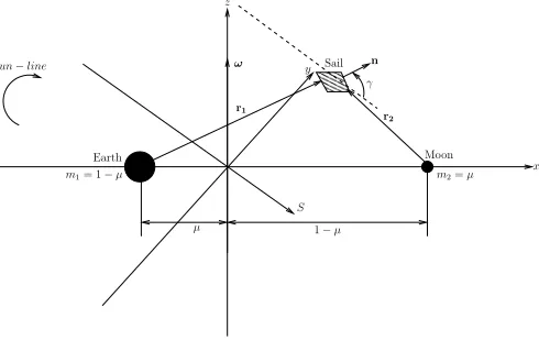
andm2=µ, withµ=m2/(m1+m2) (see Figure1). Thus, in the Earth-Moon system, the nondimensional
unit acceleration is aref =ω2R⋆ = 2.7307mm/s2 where the Earth-Moon distance R⋆ = 384400km. The
dashed line in Figure1) is a line parallel to the Sun-line directionS.
Moon
Sun−line
z
Sail
γ
n
r2 r1
x m1= 1−µ
ω
y
S
µ 1−µ
Earth
m2=µ
Figure 1. Schematic geometry of the Earth-Moon restricted three-body problem.
II.A. Equations of motion in presence of a solar sail
The nondimensional equation of a motion of a solar sail in the rotating frame of reference is described by
d2r
dt2 + 2ω×
dr
dt +∇U(r) =aS, (1)
[image:2.612.185.430.391.546.2]The three-body gravitational potentialU(r) and the solar radiation pressure accelerationaS are defined by
U(r) = − "
1 2|ω×r|
2+1−µ
r1 +
µ r2
#
,
aS = a0(S·n)2n, (2)
whereµ= 0.1215 is the mass ratio for the Earth-Moon system. The sail position vectors w.r.t. m1 andm2
respectively (see Figure 1) are r1 = [x+µ, y, z ]T andr2= [x−(1−µ), y, z]T, a0 is the magnitude of the solar radition pressure acceleration exerted on the sail and the unit vectorn denotes the thrust direction. The sail is oriented such that it is always directed along the Sun-lineS, pitched at an angleγ to provide a constant out-of-plane force. The unit normal to the sail surfacenand the Sun-line directionSare given by
n = h cos(γ) cos(ω⋆t) −cos(γ) sin(ω⋆t) sin(γ) i
T
, (3)
S = h cos(ω⋆t) −sin(ω⋆t) 0 i
T
, (4)
where ω⋆ = 0.923 is the angular rate of the Sun-line in the corotating frame in a dimensionless synodic coordinate system.
II.B. Linearized system
We now investigate the dynamics of the sail in the neighborhood of the libration points. We denote the coordinates of the equilibrium point as rL = (xLi, yLi, zLi) withi = 1,· · ·,5. Let a small displacement in rL be δrsuch that r→rL+δr.The equation of motion for the solar sail in the neighborhood of rL are therefore
d2δr
dt2 + 2ω×
dδr
dt +∇U(rL+δr) =aS(rL+δr). (5)
Then, retaining only the first-order term in δr= [ξ, η, ζ]T in a Taylor-series expansion, where (ξ, η, ζ) are attached to the L2 point as shown in Figure 1, the gradient of the potential and the acceleration can be
expressed as
∇U(rL+δr) = ∇U(rL) +∂∇U(r)
∂r
r=rL
δr+O(δr2), (6)
aS(rL+δr) = aS(rL) +∂aS(r)
∂r r=r
L
δr+O(δr2). (7)
It is assumed that∇U(rL) = 0, and the sail acceleration is constant with respect to the small displacement
δr, so that
∂aS(r)
∂r r
=rL
= 0. (8)
The linear variational system associated with the libration points atrLcan be determined by substituting Eqs. (6) and (7) into (5)
d2δr
dt2 + 2ω×
dδr
dt −Kδr=aS(rL), (9)
where the matrixKis defined as
K=−
"
∂∇U(r)
∂r r
=rL #
. (10)
Using the matrix notation the linearized equation about the libration point (Equation (9)) can be represented by the inhomogeneous linear system ˙X =AX+b(t), where the state vector X= (δr, δr˙)T, and b(t) is a
6×1 vector, which represents the solar sail acceleration. The Jacobian matrixAhas the general form
A= 03 I3
K Ω
!
whereI3is a identity matrix, and
Ω =
0 2 0
−2 0 0 0 0 0
. (12)
For convenience the sail attitude is fixed such that the sail normal vector n, points always along the direction of the Sun-line with the following constraintS·n≥0. Its direction is described by the pitch angle
γ relative to the Sun-line, which represents the sail attitude. The linearized nondimensional equations of motion relative to a collinear libration point can then be written as
¨
ξ−2 ˙η = Uo
xxξ+aξ, (13)
¨
η+ 2 ˙ξ = Uyyo η+aη, (14)
¨
ζ = Uzzo ζ+aζ, (15)
whereUo
xx, Uyyo ,andUzzo are the partial derivatives of the gravitational potential evaluated at the collinear
libration point, and the solar sail acceleration is defined in terms of three auxiliary variablesaξ,aη, andaζ
aξ = a0cos(ω⋆t) cos3(γ), (16)
aη = −a0sin(ω⋆t) cos3(γ), (17)
aζ = a0cos2(γ) sin(γ). (18)
In a similar fashion, recalling the linearized equations of motion obtained in the equation (9) describing the behavior of the system in the vicinity of the Lagrange points, it can be easily shown that the the linear variational equations of motion in component form at the triangular points then become
¨
ξ−2 ˙η = Uxxo ξ+Uxyo η+aξ, (19)
¨
η+ 2 ˙ξ = Uxyo ξ+Uyyo η+aη, (20)
¨
ζ = Uo
zzζ+aζ, (21)
We will continue with the solution to the linearized equations of motion in the Earth-Moon restricted three-body problem in the next section.
III.
Solution of the linearized equations of motion for the three-body model
In order to evaluate the three-body model, we will obtain a displaced periodic orbit from the linearized dynamics defined earlier. Considering the dynamics of motion near the collinear libration points, we may choose a particular periodic solution in the plane of the form (see Farquhar23)
ξ(t) = ξ0cos(ω⋆t), (22)
η(t) = η0sin(ω⋆t). (23)
By inserting equations (22) and (23) in the differential equations (13-15), we obtain the linear system in ξ0
andη0,
Uo xx−ω2⋆
ξ0−2ω⋆η0=a0cos3(γ),
−2ω⋆ξ0+
Uo yy−ω2⋆
η0=−a0cos3(γ).
(24)
ξ0 = a0
Uo
yy−ω⋆2−2ω⋆
cos3(γ)
Uo xx−ω2⋆
Uo yy−ω⋆2
−4ω2
⋆
, (25)
η0 = a0
−Uo
xx+ω2⋆+ 2ω⋆
cos3(γ)
Uo xx−ω2⋆
Uo yy−ω⋆2
−4ω2
⋆
, (26)
and we have the equality
ξ0
η0
= ω
2
⋆+ 2ω⋆−Uyyo −ω2
⋆−2ω⋆+Uxxo
. (27)
The trajectory will therefore be an ellipse centered on a collinear libration point. We can find the required radiation pressure acceleration by solving equation (25)
a0= cos−3(γ)
"
ω⋆4−ω2⋆(Uxxo +Uyyo + 4) +Uxxo Uyyo Uo
yy−2ω⋆−ω2⋆
#
ξ0.
By applying a Laplace transform, the uncoupled out-of-plane ζ-motion defined by the equation (15) can be obtained as
ζ(t) =U(t)a0cos2(γ) sin(γ)|Uzzo|−1+ ˙ζ0|Uzzo|−1/2sin(ωζt) + cos(ωζt)[ζ0−a0cos2(γ) sin(γ)|Uzzo|−1 (28)
where the nondimensional frequencyωζ is defined as
ωζ =|Uzzo|1/2
andU(t) is the unit step function.
A sufficient condition for displaced orbits based on the sail pitch angleγand the magnitude of the solar radiation pressurea0 for fixed initial out-of-plane distance ζ0 can be derived. Specifically for the choice of
the initial data ˙ζ0= 0,equation (28) can be more conveniently expressed as
ζ(t) = U(t)a0cos2(γ) sin(γ)|Uzzo|−1 (29)
+ cos(ωζt)[ζ0−a0cos2(γ) sin(γ)|Uzzo |−1].
The solution can then be made to contain only a constant displacement at an out-of-plane distance
ζ0=a0cos2(γ) sin(γ)|Uzzo |−1. (30)
Furthermore, the out-of-plane distance can be maximized by an optimal choice of the sail pitch angle determined by
d dγcos
2(γ) sin(γ)
γ=γ⋆
= 0,
γ⋆ = 35.264◦. (31)
We now have conditions for a small displaced periodic orbit centered on the collinear libration points.
Following the idea already presented for the collinear points, since the particular solution in the plane (Eq. (22) and (23)) cannot satisfy the linear ODEs for the triangular points (Eq. (19)-(21)), the subsequent discussion is to find solutions that satisfy these differential equations.
ξ(t) = Aξcos(ω⋆t) +Bξsin(ω⋆t), (32)
η(t) = Aηcos(ω⋆t) +Bηsin(ω⋆t), (33)
where Aξ, Aη, Bξ andBη are free parameters to be determined.
By substituting Equations (32) and (33) in the differential equations, we obtain the linear system inAξ, Aη, Bξ and Bη,
−(ω2
⋆+Uxxo )Bξ+ 2ω⋆Aη−Uxyo Bη = 0, −Uo
xyAξ+ 2ω⋆Bξ−(ω⋆2+Uxxo )Aη = 0, −(ω2
⋆+Uxxo )Aξ−Uxyo Aη−2ω⋆Bη = a0cos(γ)3,
−2ω⋆Aξ−Uo
xyBξ−(ω2⋆+Uyyo )Bη = −a0cos(γ)3.
(34)
Thus, the linear system may be solved to find the coefficientAξ, Bξ,Aη andBη, which will satisfy the ODEs.
For convenience, define
x=h Aξ Bξ Aη Bη
iT
, A=
"
A1 B1
C1 D1
#
,
and
b=h 0 0 a0cos3(γ) −a0cos3(γ)
iT
,
where the submatrices ofAare given by
A1=
"
0 −ω2
⋆−Uxxo −Uo
xy 2ω⋆
#
, B1=
"
2ω⋆ −Uxyo −ω2
⋆−Uyyo 0
#
,
C1=
"
−ω2
⋆−Uxxo 0 −2ω⋆ −Uo
xy
#
, D1=
"
−Uo
xy −2ω⋆
0 −ω⋆2−Uyyo
#
.
We have in matrix formAx=b, and the solution to the linear system is given by
x=A−1b,
where the coefficients Aξ, Aη, Bξ and Bη are amplitudes that characterize the orbit. The out-of-plane dynamics (Eq. (21)) are again uncoupled and follow the same analysis as the collinear points.
This section is now concerned with the numerical computation of displaced periodic orbits around the Lagrange points in the Earth-Moon system. As has been shown, there exist displaced orbits at all Lagrange points. For example, the numerical nonlinear results for the Lagrange points L4 (Figure 2 (a)), and L5
(Figure2 (b)) demonstrate, that displaced periodic orbits appear in their vicinity with a period of 28 days (synodic lunar month).
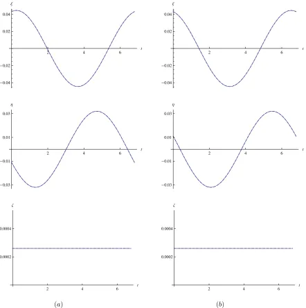
Furthermore, the numerically integrated nonlinear (solid line) equations match the linear analytic solu-tions (dashed line) for a small displaced orbit (Figure3 (a), and3(b)).
-0.04 -0.02 0.02 0.04 Ξ
-0.03 -0.02 -0.01 0.01 0.02 0.03 Η
(a)
-0.04 -0.02 0.02 0.04 Ξ
-0.03 -0.02 -0.01 0.01 0.02 0.03 Η
[image:7.612.111.517.59.212.2](b)
Figure 2. (a)Periodic Orbits at linear order aroundL4;(b)Periodic Orbits at linear order aroundL5.
2 4 6
t
-0.04
-0.02 0.02 0.04
Ξ
2 4 6
t
-0.04
-0.02 0.02 0.04
Ξ
2 4 6
t
-0.03
-0.01 0.01 0.03
Η
2 4 6
t
-0.03
-0.01 0.01 0.03
Η
2 4 6
t 0.0002
0.0004
Ζ
(a)
2 4 6
t 0.0002
0.0004
Ζ
(b)
Figure 3. (a)Comparison between the analytical (dashed line) and nonlinear (solid line) results (L4);(b)Comparison
[image:7.612.104.546.246.690.2]0.4 0.5 0.6 Ξ 0.80
0.85 0.90 0.95 1.00 Η
(a)
0.4 0.5 0.6 0.7 Ξ -0.95
-0.90 -0.85 -0.80 -0.75 -0.70 Η
[image:8.612.115.519.67.219.2](b)
Figure 4. (a)Quasi-Periodic Orbits aroundL4;(b)Quasi-Periodic Orbits aroundL5.
200 400 600 800 1000
timeHdaysL
-0.2
-0.1 0.1
Ξ
200 400 600 800 1000 timeHdaysL
-0.2
-0.1 0.1 0.2
Ξ
200 400 600 800 1000
timeHdaysL
-0.10
-0.05 0.05 0.10
Η
200 400 600 800 1000 timeHdaysL
-0.10
-0.05 0.05 0.10 0.15
Η
200 400 600 800 1000 timeHdaysL 0.000245
0.000250 0.000255 0.000260 0.000265 0.000270
Ζ
(a)
200 400 600 800 1000 timeHdaysL 0.000245
0.000250 0.000255 0.000260 0.000265 0.000270
Ζ
(b)
Figure 5. (a)Linear Feedback Control on Sailx, y, z-position (L4); (b)Linear Feedback Control on Sailx, y, z-position
[image:8.612.103.546.263.677.2]200 400 600 800 1000 timeHdaysL
-0.05 0.05 0.10
∆ΓHradsL
(a)
200 400 600 800 1000 timeHdaysL
-0.05 0.05 0.10
∆ΓHradsL
[image:9.612.101.525.58.171.2](b)
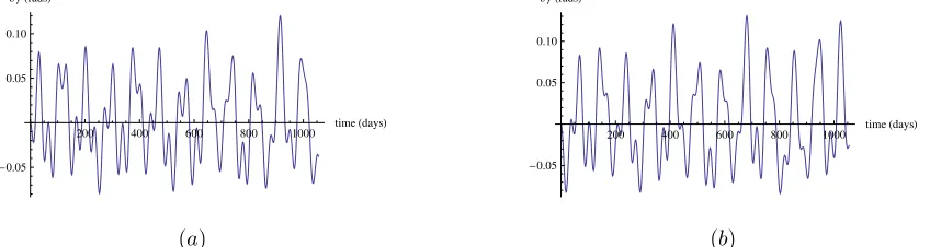
Figure 6. (a)Control History for theL4 Quasi-Periodic Orbits;(b)Control History for theL5Quasi-Periodic Orbits.
IV.
Control of Sail z-Position
In this section we consider the problem of maintaining a sail at a triangular libration point. To accomplish this task a simple control methodology is developed for stationing the solar sail. The control is achieved by using small variations in the sail’s orientation.
Recall that the motion along the z-axis is independent of the motion in the xy-plane. Thus, a z-axis control of the sail orbit is studied. Thez-position is maintained at the triangular libration points by adjusting the control angleγin such a way that it will cancell disturbances that drive the sail away from those points. The linear feedback controller is developed by linearizing thez-dynamics around the triangular libration points and some sail attitudeγ0.
From the equation (21), the linearization of the uncoupled motion aboutγ0gives
¨
ζ= ∂
2U
∂z2
o
ζ+a0cos2(γ0) sin(γ0), (35)
where the subscript o refers to the triangular libration point. If ¨ζ = 0, the condition for out-of-plane equilibrium is given by
a0cos2(γ0) sin(γ0) =−
∂2U
∂z2
o
ζ0. (36)
Now let
ζ = ζ0+δζ, (37)
γ = γ0+δγ. (38)
By making use of Eqs. (37) and (38), the uncoupled motion (Eq. (21)) can be stated as
d2
dt2
ζ0+δζ
= ∂
2U
∂z2
o
ζ0+δζ
+a0cos2(γ0) sin(γ0) +a0
cos3(γ0)−2 cos(γ0) sin2(γ0)
δγ, (39)
Applying Eq. (36), then Eq. (39) can now be rewritten as
δζ¨= ∂
2U
∂z2
o
δζ+a0
cos3(γ0)−2 cos(γ0) sin2(γ0)
δγ, (40)
whereγ06= 35.264◦.
By setting
A = ∂
2U
∂z2
o
, (41)
B = a0
cos2(γ
0)−2 cos(γ0) sin2(γ0)
Eq. (40) can also be rearranged as
δζ¨=A·δζ+B·δγ. (43)
Now it is possible to design the linear feedback controller of the form
δγ=C·δζ+D·δζ,˙ (44)
where C and D are the PD-controller gains. Thus, the PD-controller will maintain the sail at a fixed displacement above the triangular libration points.
Substituting Eq. (44) into Eq. (43), we obtain
δζ¨ = A·δζ+B(C·δζ+D·δζ˙),
= (A+BC)·δζ+D·δζ,˙ (45)
and
δζ¨−(A+BC)·δζ−D·δζ˙= 0, (46)
where D the damping coefficient is chosen such that the system converges as a critically damped system. Figure 4(a) (resp. 4(b)) shows the sail’s trajectory around L4 (resp. L5) using the linear feedback
controller on the nonlinear system. Figure5(a) (resp. 5(b)) shows the simulation results for L4 (resp. L5)
using this controller on sail x, y, z-position. The control angle history for theL4 (resp. L5) quasi-periodic
orbits is shown in Figure 6 (a) (resp. 6 (b)). It should be noted that while the z displacement is almost constant, in-plane dynamics are excited.
V.
Conclusion
Summarizing, it can be stated that, following numerical computations around the triangular libration points in the Earth-Moon system, the linear feedback controller approach based upon the z-dynamics is successful in maintaining a sail at a specific constant attitude.
As already mentioned, a sufficient condition for displaced periodic orbits based on the sail pitch angle and the magnitude of the solar radiation pressure for fixed initial out-of-plane distance has been derived.
A particular use of such orbits include continous communications between the equatorial regions of the Earth and the lunar poles.
Acknowledgments
This work was funded by the European Marie Curie Research Training Network, AstroNet, Contract Grant No. MRTN-CT-2006-035151 (J.S.) and European Research Council Grant 227571 VISIONSPACE (C.M.).
References
1
McInnes, C. R.,Solar sailing: technology, dynamics and mission applications, Springer Praxis, London, 1999, pp. 11-29.
2
Waters, T. and McInnes, C., “Periodic Orbits Above the Ecliptic in the Solar-Sail Restricted Three-Body Problem,”J. of Guidance, Control, and Dynamics, Vol. 30, No. 3, 2007, pp. 687–693.
3
Forward, R. L., “Statite: A Spacecraft That Does Not Orbit,”Journal of Spacecraft and Rocket, Vol. 28, No. 5, 1991, pp. 606–611.
4
Szebehely, V.,Therory of Orbits: the restricted problem of three bodies, Academic Press, New York and London, 1967, pp. 497-525.
5
Roy, A. E.,Orbital Motion, Institute of Physics Publishing, Bristol and Philadelphia, 2005, pp. 118-130.
6
Vonbun, F., “”A Humminbird for the L2Lunar Libration Point”,”Nasa TN-D-4468, April 1968. 7
G´omez, G., Llibre, J., Mart´ınez, R., and Sim´o, C.,Dynamics and Mission Design Near Libration Points, Vol. II, World Scientific Publishing Co.Pte.Ltd, Singapore.New Jersey.London.Hong Kong, 2001, Chaps. 1, 2.
8
G´omez, G., Jorba., A., J.Masdemont, and Sim´o, C., Dynamics and Mission Design Near Libration Points, Vol. IV, World Scientific Publishing Co.Pte.Ltd, Singapore.New Jersey.London.Hong Kong, 2001, Chap. 2.
9
11
Breakwell, J. and Brown, J., “The ‘halo’ family of 3-dimensional periodic orbits in the Earth-Moon restricted 3-body problem,”Celestial Mechanics, Vol. 20, 1979, pp. 389–404.
12
Richardson, D. L., “Halo orbit formulation for the ISEE-3 mission,” J. Guidance and Control, Vol. 3, No. 6, 1980, pp. 543–548.
13
Howell, K., “Three-dimensional, periodic, ‘halo’ orbits,”Celestial Mechanics, Vol. 32, 1984, pp. 53–71.
14
Howell, K. and Marchand, B., “”Natural and Non-Natural Spacecraft Formations Near L1 and L2 Libration Points
in the Sun-Earth/Moon Ephemerics System”,” Dynamical Systems: An International Journal, Vol. 20, No. 1, March 2005, pp. 149–173.
15
McInnes, C., “Solar sail Trajectories at the Lunar L2Lagrange Point,”J. of Spacecraft and Rocket, Vol. 30, No. 6, 1993,
pp. 782–784.
16
Ozimek, M., Grebow, D., and Howell, K., “Solar Sails and Lunar South Pole Coverage,”In AIAA/AAS Astrodynamics Specialist Conference and Exhibit, AIAA Paper 2008-7080, Honolulu, Hawaii, August 2008.
17
Baoyin, H. and McInnes, C., “Solar sail halo orbits at the Sun-Earth artificial L1 point,” Celestial Mechanics and
Dynamical Astronomy, Vol. 94, No. 2, 2006, pp. 155–171.
18
Baoyin, H. and McInnes, C., “Solar sail equilibria in the elliptical restricted three-body problem,”Journal of Guidance, Control and Dynamics, Vol. 29, No. 3, 2006, pp. 538–543.
19
Baoyin, H. and McInnes, C., “Solar sail orbits at artificial Sun-Earth Lagrange points,”Journal of Guidance, Control and Dynamics, Vol. 28, No. 6, 2005, pp. 1328–1331.
20
McInnes, C. R., “Artificial Lagrange points for a non-perfect solar sail,”Journal of Guidance, Control and Dynamics, Vol. 22, No. 1, 1999, pp. 185–187.
21
McInnes, C., McDonald, A., Simmons, J., and McDonald, E., “Solar sail parking in restricted three-body systems,”
Journal of Guidance, Control and Dynamics, Vol. 17, No. 2, 1994, pp. 399–406.
22
Simo, J. and McInnes, C. R., “Solar sail trajectories at the Earth-Moon Lagrange points,”In 59th International Astro-nautical Congress, IAC Paper 08.C1.3.13, Glasgow, Scotland, 29 September - 03 October 2008.
23