High-order wavelet reconstruction for multi-scale edge aware tone mapping

High-Order Wavelet Reconstruction for Multi-Scale Edge Aware Tone Mapping

Alessandro Artusia_{, Zhuo Su}b,c_{, Zongwei Zhang’s}b,c_{, Dimitris Drikakis}d_{, Xiaonan Luo}b,c

a_{Graphics and Imaging Laboratory Department of Informatics and Applied Mathematics University of Girona.} b_{National Engineering Research Center of Digital Life, Guangzhou, China.}

c_{School of Information Science and Technology, Sun Yat-sen University, Guangzhou, China.} d_{Fluid Mechanics and Computational Science Cranfield University.}

Abstract

This paper presents a High Order Reconstruction (HOR) method for improved multi-scale edge aware tone map-ping. The study aims to contribute to the improvement of edge-aware techniques for smoothing an input image, while keeping its edges intact. The proposed HOR methods circumvent limitations of the existing state of the art meth-ods, e.g., altering the image structure due to changes in contrast; remove artefacts around edges; as well as reducing computational complexity in terms of implementation and associated computational costs. In particular, the proposed method aims at reducing the changes in the image structure by intrinsically enclosing an edge-stop mechanism whose computational cost is comparable to the state-of-the-art multi-scale edge aware techniques.

Keywords:

1. Introduction 1

High Order Reconstruction (HOR) methods, intro-2

duced by Harten et al. [1], have been used exten-3

sively for solving the hyperbolic conservation laws and 4

the Hamilton-Jacobi equations [2]. Additionally, these 5

methods have been applied to image processing (image 6

compression), denoising [3] and segmentation [4]. Due 7

to their ability to reduce oscillations around function 8

discontinuities, these methods can be potentially used 9

as an edge aware interpolation tool. Edge-aware tech-10

niques such as anisotropic di↵usion [5], bilateral

filter-11

ing [6, 7] and neighborhood filtering rely on sophisti-12

cated type of spatially varying kernels. Often, they tend 13

to either generate artificially staircasing e↵ects or

ring-14

ing e↵ects around sharp edges [8]. These artifacts can

15

be reduced using a post-processing step at the price of 16

increasing the computational cost and the number of pa-17

rameters used [9]. To have better control of the details 18

over the spatial scale, one can apply edge-aware tech-19

niques in a multi-scale fashion. However, the bilateral 20

filtering is inappropriate for multi-scale detailed decom-21

position [10]. Other edge-aware techniques that sup-22

port the multi-scale approach [10, 11, 9] also encompass 23

some flaws, e.g., they are not able to achieve a plausible 24

reproduction of all important image features [12] and 25

may change the image structure. 26

Therefore, there is a need to develop methods that are 27

reducing as much as possible any change into the image 28

structure without increasing the complexity or compu-29

tational cost. 30

In this paper, we link the edge-aware problem to the 31

typical problem of interpolation. In particular, we pro-32

pose a novel wavelet scheme that uses a robust predictor 33

operator, based on the HOR method, which intrinsically 34

encloses an edge-stop mechanism to avoid influence of 35

pixels from both sides of an edge. To have a better con-36

trol of details over the spatial scale, we employ the HOR 37

method in conjunction with a multi-scale scheme. 38

We demonstrate the usability of the proposed method to 39

solve a typical problem in the context of High Dynamic 40

Range (HDR) imaging, called tone mapping as defined 41

in Banterle et al. [13]. 42

The approach is formulated as follows; we decom-43

pose an input HDR image, making use of wavelet de-44

composition and through the use of HOR methods sep-45

arate its coarse and fine features (details). The coarse 46

and fine features are then manipulated to achieve the de-47

sired tone and details levels. Finally, the output image 48

is reconstructed. The advantage of the above approach 49

is that it does not require the introduction of any edge-50

stopping function that limits possible image-structure 51

changes. 52

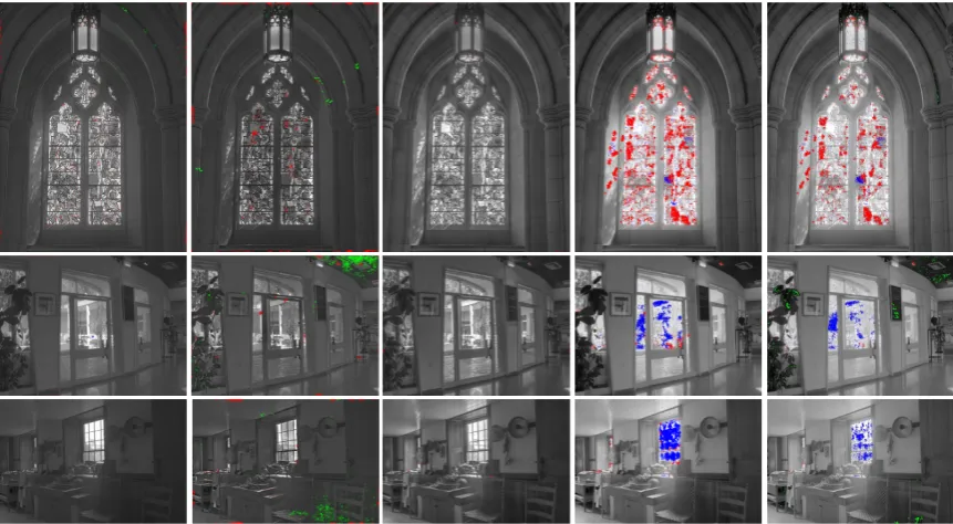
To understand this concept, Figure 1 shows the dis-53

Figure 1: Comparison of the state-of-the-art multiscale edge aware based tone mapping operators and the present HOR: 1st_{row: output of the}

various techniques. 2nd _{row: distortion map of the DRIM metric [12]. This map is showing the pixels that shows a distorsion with 95% of}

probability to been seen by the Human Visual System (HVS). Blue pixels are areas where invisible contrast is introduced; red pixels are areas where reversal of visible contrast is noticeable and green pixels shows areas of lost of contrast. The map is showing of a reduction of more than 50% of the pixels a↵ected by loss of contrast when the the HOR method is used. Parameters used - Farbmann et al. [10] multiscale approach balanced - Fattal’s [11]↵=0.9, =0.16 and =0.8 - Paris et al. [9] r=log(2.5),↵=0.5 and =0.0 (for conveying the local e↵ect) - The Present HOR =0.7, =0.9.

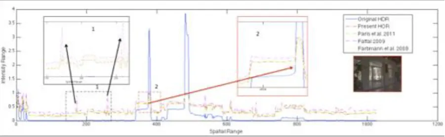
Figure 2: Intensity profile for the tone mapping operators on an HDR mage for line 300: The 1st_{zoomed area, clearly shows how Fattal’s [11]}

method (undesirably) increases the intensity profile to the maximum value of 1. In the 2nd_{zoomed area (Paris et al. [9] green line), the intensity}

dent metric (DRIM) introduced by Aydin et al. [12] for 55

[10, 11, 9] and the technique proposed in this paper. The 56

original HDR image is used as reference, and the output 57

of the tone mapping operator is compared to it. A cer-58

tain amount of lost of contrast (green) is clearly visible, 59

and this may change the overall image structure [12]. 60

The map shows that using the present HOR reduces the 61

number of pixels a↵ected by loss of contrast by more

62

than 50%. 63

Moreover, the intensity profile may change as shown 64

in Figure 2. The Fattal method [11] may have an un-65

desirable increase of the intensity profile to the maxi-66

mum output value 1 (1st_{zoomed area). The structure of} 67

the original profile may be undesirably modified (green 68

line) as shown for the method [9] (2nd _{enlarged area).} 69

These methods may result in prohibitive computational 70

costs (see Paris et al. [9]). An efficient

implementa-71

tion [14] of the method presented by Paris et al. [9] 72

is also discussed in Section 6. 73

The proposed approach retains the same advantages 74

introduced by the traditional edge aware approaches 75

such as Paris et al. [9], and Fattal [11], namely with re-76

spect to obtaining local properties and providing robust 77

smoothing, hence avoiding the use of pixels from both 78

sides of the edge. The main contributions of this work 79

can be summarized as follows: 80

1. Establish a link between the robust smoothing 81

concept to the reconstruction problem of a non-82

smoothed function. 83

2. Achieve a complex solution of the edge-aware 84

problem, through a simple and flexible point-wise 85

manipulation by using HOR method. 86

3. Propose an edge-aware filter that produces halo 87

free results; reduces the changes in the image 88

structure as defined by the DRIM metric and its 89

computational cost is increasing linearly with re-90

spect to the number of the input pixelsN. 91

2. Related Work 92

Edge Aware Filters 93

Edge aware techniques are used to smooth an image 94

while keeping its edges intact, preventing pixels located 95

on one side of a strong edge from influencing pixels on 96

the other side. This concept can be used to separate high 97

frequency information from low frequency information 98

such as texture and details. Once this separation is pe-99

formed the high and low frequencies information can be 100

independently manipulated and re-composed. 101

In the past, techniques able to preserve edges [6, 8, 5] 102

have been applied to image manipulation [15, 16, 17, 103

11]. These techniques produce acceptable results, but 104

often introduce visible ringing e↵ects arising from the

105

Poisson equation [15] and filtering, as discussed in [10, 106

8]. Moreover, they need several parameters, that are im-107

age dependent, making their set-up difficult for

practi-108

cal applications [17]. Our approach o↵ers a solution,

109

that produces results at least as good as the above tech-110

niques, runs linearly in time with respect to the number 111

of the input pixels and is not dependent on a large num-112

ber of parameters. 113

Multi-Scale Edge Aware Filters 114

Recently, several edge-aware techniques that can be 115

used in the multi-scale framework, have been presented. 116

Typically, these methods exploit the multi-scale ap-117

proach by making use of pyramid mechanisms such as 118

Laplacian [18], Gaussian [19], and Wavelets [20]. 119

The Laplacian approach, in the context of edge-aware, 120

has been recently revised by Paris et al. [9] through the 121

use of local transformation which makes the Laplacian 122

approach suitable for edge-aware operations. Farbman 123

et al. [10] employed the weighted least square to build 124

an alternative edge preserving operator and extend it to 125

multi-scales as well. Fattal et al. [15] used the Gaus-126

sian Pyramid to compress the high dynamic range of the 127

input image, followed by the full image reconstruction 128

through the use of the Poisson solver. 129

The aforementioned techniques share with our ap-130

proach the multi-scale ’philosophy’, but are using dif-131

ferent methods such as the Laplacian [10, 9] and Gaus-132

sian [15] pyramids. Moreover, they are based on the so-133

lution of a linear system [10], a Poisson solver [15], or 134

bilateral filtering all of which generate artifacts around 135

edges [8]. Li et al. [21] proposed a multi-scale approach 136

based on wavelets where each sub-band signal is mod-137

ified using a gain map that controls the local contrast. 138

Fattal [11] presented an edge avoiding technique based 139

on a second generation wavelet. Our approach inte-140

grates within the wavelet mechanism a HOR technique 141

that does not require any edge-stop function for com-142

puting a large set of weights in the interpolation step 143

as in [11]. Consequently, using the present approach 144

there is no need for any particular precaution against 145

the strong edges and distortions of the image structure 146

are reduced. 147

3. Background 148

Fixed stencil approximation techniques, such as 149

piecewise linear and cubic interpolation, are often used 150

to reconstruct the missing points of a function. These 151

methods are working well in the case where the func-152

Figure 3: Example of the HOR scheme mechanism. (Top row) The original staircase signal. (2nd_{row) The uniform grid points: (circle}

red) input points, (square blue) points to be interpolated. (3rd_row)

The stencil points used by the HOR scheme. (4th _{and 5}th _rows):

Two separated stencils used to define the two interpolants by the HOR scheme.

wise smooth the fixed stencil approximation may not be 154

adequate near discontinuities. In fact, oscillations at the 155

function discontinuities are visible, 156

Essential Non-oscillatory Scheme 157

Essential Non-oscillatory Schemes (ENO) have been in-158

troduced by Harten et al. [1] to solve this problem. The 159

ENO scheme makes use of adaptive stencils, thus the 160

use of discontinuity cells is avoided. Let us consider a 161

signal function f(x) with given grid of points of evalu-162

ated values such asv[i]= f[xi]. 163

The ENO scheme reconstructs f from the point values 164

vassuming that f is piecewise polynomial. This means 165

that for each cell Ii ⌘ [xi 1,xi+1] a polynomial

inter-166

polantpi(x) is defined using the set of points defined in 167

the stencilSi. The idea is to find a stencil ofk+1 con-168

secutive points, includingxi 1andxi+1, where the signal 169

f(x) is the smoothest in this stencil when comparing it 170

with the other possible stencils. To evaluate the smooth-171

ness of f(x) we can use the Newton divide di↵erences

172 of f: 173

f[x0]⌘f(x0); f[x0,x1]⌘₍xf0[x0]x1)+

f[x1] (x1 x0); ...

(1) 174

In general, the j-thdegree divided di↵erence of f(x)

175

is equivalent to 176

f[xi 1, .,xi+j 1]⌘

f[xi, .,xi+j 1] f[xi 1, .,xi+j 2]

xi+j 1 xi 1

.(2) 177

Starting from a two points stencil 178

S2(i)=xi 1,xi+1, (3) 179

the linear interpolation of the stencil S2 in a Newton 180

form is 181

p1(x)= f[xi 1]+f[xi 1,xi+1](x xi 1). (4)

182

To expand the stencil we have two possibilities, either 183

add the left neighborxi 2or the right onexi+2. In both

184

cases this will be a quadratic interpolation polynomial. 185

This will di↵er from the linear polynomial of eq. 4, by

186

the same function multiplied by two di↵erent constants.

187

These constants are the two 2-nddegrees of divided dif-188

ferences of f(x) in two di↵erent stencils defined by the

189

left and right neighbors.This procedure is continued un-190

til thek+1 points in the stencil are reached. 191

High Order Interpolation Scheme (HOR) 192

The typical problem of the ENO scheme is that it 193

can exhibit oscillatory behavior and is also fairly ex-194

pensive in its implementation [22]. As an alterna-195

tive, the weighted ENO (WENO) variant has been pro-196

posed1_{. WENO uses a convex combination of all the} 197

corresponding interpolating polynomials on the stencil 198

to compute an approximated polynomial for each cell 199

(Figure 3). A convex combination is a linear combina-200

tion where the coefficients (weights) are all positive and

201

their sum is equal to 1. The key points of the reconstruc-202

tion scheme are (at 3rd_{order accuracy):} 203

1. Stencils definition: Taking a cell defined in the in-204

terval [xi 1/2,xi+1/2] (see Figure 3), the stencils are 205

defined as [22] 206

S1=(xi 3/2,xi 1/2,xi+1/2);

S2 =(xi 1/2,xi+1/2,xi+3/2) (5) 207

2. Interpolation polynomials: For each stencil the lin-208

ear interpolation polynomial is computed as 209

p1= f[xi]+ f[xi] f_x[xi1](x xi);

p2= f[xi]+ f[xi+1]_xf[xi](x xi) (6) 210

where the f[x] elements are the available data 211

points of the function to be reconstructed (red 212

points in Figure 3). 213

3. Convex combination: The interpolation polynomi-214

als are combined following a convex combination 215

Pi= a i 0 ai

0+ai1

p1+ a i 1 ai

0+ai1

p2 (7)

216 where 217 ai 0= Ci 0 (✏+(IS)1)2.0;

ai 1=

Ci

1 (✏+(IS)2)2.0

(8) 218

1_{WENO schemes have been widely used in computational fluid}

Figure 4: Overview of the present approach. Firstly, a pyramid repre-sentation of the input HDR image is produced using a forward wavelet lifting scheme with integrated the HOR interpolation method pre-sented in this paper. Secondly, the coarse level of the pyramid struc-ture (blue continue arrow) and the details levels (blue dashed arrows) are manipulated. Thirdly, the modified pyramid is collapsed to recon-struct the output tone mapped image. This is done, using the backward wavelet lifting scheme with integrated the HOR interpolation model.

IS are the smoothness indicators, which are calcu-219

lated as (IS)1 = (f[xi] f[xi 1])2.0 and (IS)2 = 220

(f[xi+1] f[xi])2.0. The gradient magnitude is well

221

known to be a good estimator of edge information. 222

Based on this observation, we have used the im-223

age gradient to select the coefficients C as given

224

by [22], allowing the interpolation step to be aware 225

of edge information in order to avoid an edge-226

stopping function. 227

• @E(f)/@f >0:C₀i =1/2 andCi₁=1; 228

• @E(f)/@f <0:C₀i =1 andCi₁=1/2. 229

4. HOR Wavelet Scheme 230

In this paper we propose a robust smoothing through the 231

use of a polynomial interpolant that makes use of the 232

smoothest stencils. It is integrated in a wavelet scheme 233

(lifting scheme) to take advantage of the multi-scale 234

representation such as the capability to retain image in-235

formation at di↵erent scale. Figure 4 shows the

princi-236

ple of the present approach. Firstly, a pyramid repre-237

sentation of the original input imageI is produced us-238

ing a forward wavelet lifting WENO scheme. Secondly, 239

the coarse (blue continued arrows) and fine levels (blue 240

dashed arrow) are manipulated. Thirdly, the modified 241

multiscale representation is collapsed to the output im-242

age using the backwards wavelet lifting WENO scheme. 243

A multi-scale representation can be obtained by making 244

use of a nested series of decimationDand reconstruc-245

tionRoperators. As aDoperator, we have used a simple 246

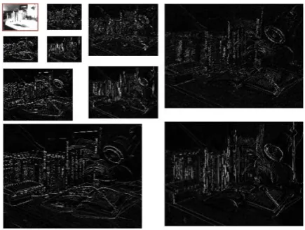
Figure 5: Pyramid image representation, after having applied the for-ward wavelet lifting WENO scheme. The coarse level is the image at the upper left corner (with red frame). The other images are repre-senting the details, at di↵erent levels, for the horizontal, diagonal and vertical directions.

splitting operation which separates the pixels of the in-247

put at levelkin two di↵erent grids based on the index

248

number (odd and even). For theRoperator the WENO 249

scheme has been employed according to which the level 250

kis reconstructed fromk+1 using eq. 9: 251

˜

Ik_[x,y]=w

0[x,y](Ik+1[x 1,y]+ Ik+1_{[x 1,y] I}k+1_{[x 3,y]}

[x 1,y] [x 3,y] ([x,y] [x 1,y])) +w₁[x,y](Ik+1_{[x 1,y]+} Ik+1_{[x+1,y] I}k+1_{[x 1,y]}

[x+1,y] [x 1,y] ([x,y] [x+1,y])).

(9) 252

Eq. 9 is equivalent to eq. 7 where w0 and w1 are its 253

factorial terms.The di↵erence in the indices between

254

eq. 9 and eq. 7 is due to the fact that we have inserted 255

zero pixels at k+1 level and would like to retain in-256

teger numbers in the indexing of the grid. Fattal [11] 257

presented a robust average operator, for both type of 258

wavelet approaches, red black and weighted CDF, 259

making use of an edge stop function to compute the 260

prediction weights. In our case, as described ineq.7, 261

we present a convex combination of polynomial inter-262

polants. However, these polynomial interpolants are lin-263

ear, thus we can consider the overall operator as a com-264

bination of linear interpolants. 265

At the boundaries of the input image, we have 266

adopted a standard extrapolation approach to generate 267

the missing values in the stencil . The restored ˜Ik_level 268

is later used to obtain the details of the k+1 level 269

dk+1_=Ik _I˜k_{. To preserve the overall sum of the coarse}

270

elementsIk+1, and based on the fact that the operatorR 271

we have decided to use a linear interpolator as update-273

operatorU: 274

U(dk+1_)[x,y]= dk+1[x 1,y]+dk+1[x+1,y]

4 ;(10)

275

and the levelk+1 of coarse elements is updated using 276

Ik+1_=Ik+1_+U(dk+1_). 277

This process is repeated both for the rows and 278

columns of the input image. 279

Discussion An example of the behaviour of the 280

present HOR, integrated in the wavelet scheme, is 281

shown in Figure 5. The coarse,c, and ’details’ coeffi

-282

cients, d, (vertical, diagonal and horizontal) for three 283

levels are shown. Edges are detected by the wavelet 284

scheme avoiding the influence of pixels on both sides 285

at each scale. This is obtained without the introduction 286

of an edge stop function utilized for the computation of 287

the set of weights used in the interpolation step as pro-288

posed by Fattal [11] . 289

5. Tone Mapping Manipulation 290

In this subsection, we will show how to make use 291

of the proposed technique in the classical tone ma-292

nipulation problem. Tone manipulation allows to re-293

duce the intensity of the luminance range of HDR con-294

tent. This objective is achieved through compression of 295

large-scale variation and keeping the fine level informa-296

tion. The filtering approach is applied to the natural log-297

arithmic scale of the luminance, keeping the color ratio 298

unaltered as in Paris et al. [9], using a gamma correction 299

of 2.2. 300

To manipulate the tone and the details of the input HDR 301

image, we have followed a similar approach to the one 302

used by Fattal [11]. The tone is linearly manipulated 303

modifying the coarse coefficientcof the coarsest leveln

304

through a parameter , as cn_{. This allows us to achieve} 305

the compression of the vast dynamic range available in 306

the input HDR image. A second parameter is used 307

to manipulate the details. This is obtained from the 308

progressive decreasing of the ’details’ coefficientsdk,

309

such as k_dk_{wherekis the number of levels varying} be-310

tween 1 ton. The and parameters are in the range of 311

(0.0,1.0]. 312

Since our approach shares several aspects with the tech-313

nique presented by Fattal [11], we first provide an anal-314

ysis and comparison to show how the present technique 315

performs with respect to the preservation of edges, 316

while at the same time adjusting the tone of the input 317

image. 318

Figure 6: Comparisons with state-of-the-art method Fattal’s method [11] . 1st_{row: Fattal [11] using wavelet Red and Black model}

with↵=0.8, =0.11 and =0.68 - 2nd_{row: the present approach}

with =0.3 and =0.7 -2nd_{column: Gradient of a zoomed area, it}

showing the degree of edge preservation.

Figure 7: Comparisons of di↵erent methods. 1stcolumn: Fattal [11] using wavelet Red and Black model with parameters as per web project page [26] - 2nd_{column: The present approach with =0.7}

and =0.9 - 2nd_{row: Gradient of the zoomed area in the 3}rd_row.

(a) Fattal [11] =0.7 - Weak (b) Fattal [11] =0.5 - Strong

Figure 8: Results from the application of Fattal’s et al. [11] tech-nique making use of the new contractive concave mapping as specified in [26].

The present technique produces results comparable 319

to this state-of-the-art operator, while o↵ering the

ad-320

vantage of not using an extra edge-stop function. The 321

technique of [11] is capable to capture more details but 322

at the cost of introducing some distortions at the edge 323

level, as shown in Figures 7 (a) (zoomed lamp area and 324

its edge map) and 6 (b) (edge map). 325

One may reduce these distortions by making use of a 326

new compression technique, as suggested in [26] (Fig-327

ure 8 ). However, artifacts may appear as shown in Fig-328

ure 8 (b) 2nd _row. 329

6. Experimental Results 330

The HOR approach has been implemented in Matlab 331

and the experiments have been performed on a Mack-332

book air with Intel i7-core CPU 1.8 GHz, 64-bit ma-333

chine and 4GB of RAM. We have compared our tech-334

nique with the latest edge aware state-of-the-art multi-335

scale approaches, applied to the tone mapping problem, 336

such as[11, 9, 10]. We have used the Matlab code as 337

well as parameters provided by the authors. 338

We have chosen the set of images shown in Figure 9. 339

This set consists of 18 images with di↵erent dynamic

340

range that span from outdoor to indoor and from light to 341

dark illumination conditions. 342

Figure 9: Images used in the experiments. The numbering in Tables 1 and 2 follows the order of the images from the top to the bottom and from the left to the right.

6.1. Quality 343

To provide a fair comparison, we have selected the 344

parameters of the di↵erent techniques to convey

sim-345

ilar appearance in term of contrast, edges and details 346

preservation to all the techniques presented in this com-347

parison. 348

We may observe that the DRIM metric is measur-349

ing changes in contrast, in other words the overall ap-350

pearance of the image, and it is not able to detect if 351

small-scale details are not well preserved. On the other 352

hand, edge-aware techniques are able to preserve well 353

small-scale details. This is preserved intrinsically by the 354

mechanisms described in the previous sections as well 355

as by the results shown here that are comparable with 356

the existing state-of-the-art edge aware technique [11]. 357

Based on the fact that small-scale details are to certain 358

extent well reproduced by the edge-aware techniques, 359

our objective was to examine how these techniques are 360

able to convey the overall appearance of the input HDR 361

into the tone mapped result. In doing so, we have de-362

cided to use the DRIM metric as specified below. 363

Since the DRIM metric acceptscd/m2_{values, the} in-364

put images need to be calibrated. In the case of the tone 365

mapped input image, we need to linearize the input sig-366

nal and then map it to the dynamic range of the display 367

where the image will be visualized. In our case, the 368

value used for the linearization step is 2.2, and the dy-369

namic range chosen is [0.5, 100] cd/m2 _{. In the case} 370

of the HDR input image, there was no need to linearize 371

the signal, and the dynamic range has been chosen as 372

[0.015, 3000]cd/m2_. 373

Figure 10: Output and DRIM comparison with state-of-the-art edge aware approaches.1st_{- row output of the edge aware technique; 2}nd_row

-DRIM metric [12] with probability of 75%; 3rd_{row - DRIM metric [12] with probability of 95%. Parameters used - Farbmann et al. [10] multiscale}

approach balanced - Fattal’s [11]↵=0.9, =0.19 and =0.5 - Paris et al. [9] r=log(2.5),↵=0.5 and =0.0 (for conveying the local e↵ect) -The Present HOR =0.7, =0.9.

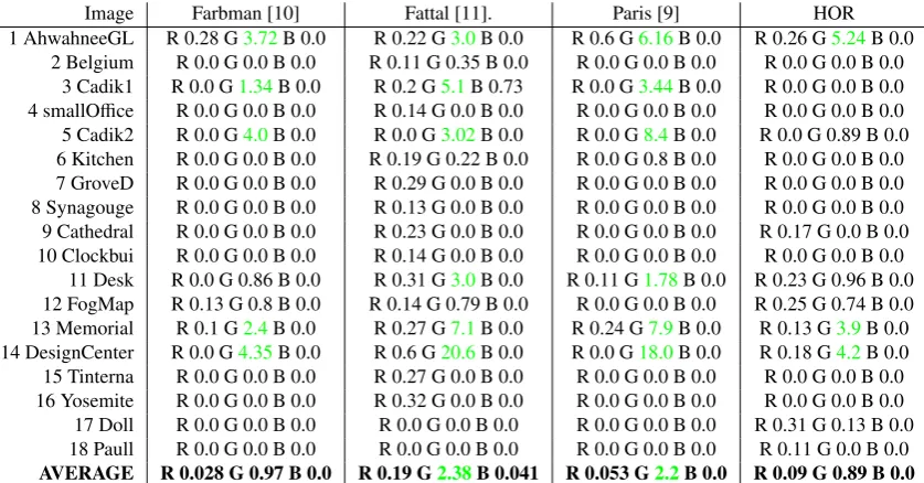
Tables 1 and 2 show the results of the DRIM metric 375

applied to the test set images. The numbers represent 376

the percentage of pixels with probability for the distor-377

tion to be perceived by the HVS. Tables 1 and 2 show 378

the results with probability 95% and 75%, respectively. 379

The colors used to depict the type of distortion are the 380

same with those used to describe the distortion -R(red) 381

reversal, -G(green) lost and -B(blue) amplification of 382

contrast. We have colored the methods that show the 383

higher probability, as well as the ones that show signifi-384

cant percentage of pixels with the specified probability. 385

In the case of probability 95%, the significant distortion 386

introduced by the state-of-the-art edge aware methods, 387

as well as by the present HOR is mostly due to the loss 388

of contrast; neither reversal nor amplification of con-389

trast are significant. The lost of contrast is attributed to 390

the fact that the edge-aware methods are using simple 391

linear scaling for compressing the large luminance dy-392

namic range. This may a↵ect the overall preservation of

393

local contrast. With probability 95% the state-of-the-art 394

methods may present high percentage of pixels a↵ected

395

by loss of contrast. This is the case of the images 1, 3, 396

5, 11,13 and 14. In most of the other cases, this number 397

is negligible. For the images 1, 13 and 14, the HOR 398

shows a slightly higher percentage value for the loss 399

of contrast. However, this value is either comparable 400

or lower than the value provided by the state-of-the-art 401

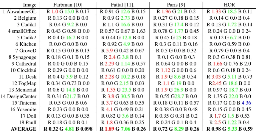
edge-aware methods.We have also tried to analyze the 402

results of the DRIM metric at lower probability such 403

as 75% and the results are shown in Table 2. As ex-404

pected, the percentage of pixels is drastically increased 405

and more images are a↵ected by a significant

percent-406

age value. In this case, reversal of contrast (red) and in 407

some cases amplification of contrast (blue) may appear. 408

In the case of loss of contrast the Fattal [11] and Paris et 409

al. [9] results show that the majority of the images are 410

a↵ected by this type of distortion. This type of

distor-411

tion also a↵ects the present HOR, but when compared

412

with the state-of-the-art edge-aware methods shows a 413

lower percentage of pixels a↵ected by this distortion.

414

Only in the case of image 18 the present HOR shows 415

higher value for the loss of contrast. However, this per-416

centage value is quite small and it is not actually per-417

ceivable by the HVS. The results are also a↵ected by

418

the reversal of contrast. In particular, several results 419

of Fattals [11] method are showing this distortion. The 420

present HOR shows reversal of contrast higher than the 421

other methods only for three images (11, 12 and 18). 422

Finally, the amplification of contrast (blue) does almost 423

not exist, and the only image that is a↵ected by using

424

the proposed HOR is the image 15. 425

DRIM Visual Analysis 426

Figures 10, 11, 13 and 14 show results with the 427

corresponding DRIM distortion maps. Figure 10 and 428

Figure 11 compares the DRIM maps at probability 75% 429

Figure 11: Output and DRIM comparison with state-of-the-art edge aware approaches.1st_{- row output of the edge aware technique; 2}nd_row

-DRIM metric [12] with probability of 75%; 3rd_{row - DRIM metric [12] with probability of 95% (for both images). Parameters used - Farbmann et}

Image Farbman [10] Fattal [11]. Paris [9] HOR 1 AhwahneeGL R 0.28 G3.72B 0.0 R 0.22 G3.0B 0.0 R 0.6 G6.16B 0.0 R 0.26 G5.24B 0.0

2 Belgium R 0.0 G 0.0 B 0.0 R 0.11 G 0.35 B 0.0 R 0.0 G 0.0 B 0.0 R 0.0 G 0.0 B 0.0 3 Cadik1 R 0.0 G1.34B 0.0 R 0.2 G5.1B 0.73 R 0.0 G3.44B 0.0 R 0.0 G 0.0 B 0.0 4 smallOffice R 0.0 G 0.0 B 0.0 R 0.14 G 0.0 B 0.0 R 0.0 G 0.0 B 0.0 R 0.0 G 0.0 B 0.0 5 Cadik2 R 0.0 G4.0B 0.0 R 0.0 G3.02B 0.0 R 0.0 G8.4B 0.0 R 0.0 G 0.89 B 0.0 6 Kitchen R 0.0 G 0.0 B 0.0 R 0.19 G 0.22 B 0.0 R 0.0 G 0.8 B 0.0 R 0.0 G 0.0 B 0.0 7 GroveD R 0.0 G 0.0 B 0.0 R 0.29 G 0.0 B 0.0 R 0.0 G 0.0 B 0.0 R 0.0 G 0.0 B 0.0 8 Synagouge R 0.0 G 0.0 B 0.0 R 0.13 G 0.0 B 0.0 R 0.0 G 0.0 B 0.0 R 0.0 G 0.0 B 0.0 9 Cathedral R 0.0 G 0.0 B 0.0 R 0.23 G 0.0 B 0.0 R 0.0 G 0.0 B 0.0 R 0.17 G 0.0 B 0.0 10 Clockbui R 0.0 G 0.0 B 0.0 R 0.14 G 0.0 B 0.0 R 0.0 G 0.0 B 0.0 R 0.0 G 0.0 B 0.0

11 Desk R 0.0 G 0.86 B 0.0 R 0.31 G3.0B 0.0 R 0.11 G1.78B 0.0 R 0.23 G 0.96 B 0.0 12 FogMap R 0.13 G 0.8 B 0.0 R 0.14 G 0.79 B 0.0 R 0.0 G 0.0 B 0.0 R 0.25 G 0.74 B 0.0 13 Memorial R 0.1 G2.4B 0.0 R 0.27 G7.1B 0.0 R 0.24 G7.9B 0.0 R 0.13 G3.9B 0.0 14 DesignCenter R 0.0 G4.35B 0.0 R 0.6 G20.6B 0.0 R 0.0 G18.0B 0.0 R 0.18 G4.2B 0.0 15 Tinterna R 0.0 G 0.0 B 0.0 R 0.27 G 0.0 B 0.0 R 0.0 G 0.0 B 0.0 R 0.0 G 0.0 B 0.0 16 Yosemite R 0.0 G 0.0 B 0.0 R 0.32 G 0.0 B 0.0 R 0.0 G 0.0 B 0.0 R 0.0 G 0.0 B 0.0 17 Doll R 0.0 G 0.0 B 0.0 R 0.0 G 0.0 B 0.0 R 0.0 G 0.0 B 0.0 R 0.31 G 0.13 B 0.0 18 Paull R 0.0 G 0.0 B 0.0 R 0.0 G 0.0 B 0.0 R 0.0 G 0.0 B 0.0 R 0.11 G 0.0 B 0.0 AVERAGE R 0.028 G 0.97 B 0.0 R 0.19 G2.38B 0.041 R 0.053 G2.2B 0.0 R 0.09 G 0.89 B 0.0

Table 1:DRIM results over the set of images presented in Figure 9. We show the percentage of pixels with probability of 95% that present the distortion of reverse (R), loss (G), or amplification (B) of contrast.

The visual analysis of the results shows that in the 431

case of probability 75% the state-of-the-art methods 432

show a consistent number of distorted pixels localized 433

in large areas, when compared with the present HOR. 434

On the other hand, when the probability increases to 435

95%, the size of these areas are either reduced or are 436

almost not a↵ected by any distortion. However, in some

437

cases the state-of-the-art methods are still showing large 438

areas of lost of contrast (green) and reversal of contrast 439

(red). 440

Figures 13 and 14 are showing other results with the 441

distortion maps with probability at 95%, where the all 442

methods are showing similar behavior.. 443

Comparison with Simpler TMO’s 444

One can observe that the global operators are faster 445

and convey an overall better appearance (Artusi et 446

al. [28]). For this purpose, we have computed the 447

DRIM maps for a well known global version of two 448

TMOs published by by Reinhard et al. [27] and Drago 449

et al. [27]. The comparison is limited to the global op-450

erator showing that the quality of the results is not com-451

parable with the state-of-the-art edge aware techniques. 452

The results are shown in Figure 12 for the distortion 453

maps at probability of 95%. 454

The results reveal that the DRIM obtained for the 455

Reinhard et al. [27] and the Drago et al. [27] opera-456

tors often show larger areas of amplification of contrast; 457

see the window area in Figure 12, in comparison with 458

the results obtained by the majority of the edge-aware 459

techniques employed in this experiment. 460

Figure 12 (2n_{d row shows reversal of contrast, in} 461

large areas of the window, for both global operators. 462

On the other hand, the edge-aware techniques have very 463

tiny areas a↵ected by reversal of contrast. Moreover,

464

we emphasize in general that global operators are not 465

designed for edge-awareness and do not encapsulate 466

mechanisms for retaining the fine details at di↵erent

467

spatial scale, as in the case of the present HOR and 468

edge-aware techniques. 469

6.2. Computational Analysis 470

Another aspect that needs to be taken into account 471

is the computational cost associated with the di↵erent

472

algorithms. Here, we have performed a computational 473

cost analysis for the proposed technique versus other 474

state-of-the-art techniques. 475

Our approach presents computational complexity and 476

associated cost comparable to the one presented in [11, 477

10] and outperforming the method of [9] . 478

Specifically, the method presented by Paris et al. [9] 479

requires 1738 sec to process an image size of 800x525, 480

420 sec for an image size of 400x262 and 190 sec. for 481

an image size of 267x174. When compared with the 482

computational cost of our method and the approaches 483

of [11, 10], the computational cost is significantly re-484

duced: 14 sec to process an image size of 800x525, 3 485

sec for an image size of 400x262, and 1 sec for an im-486

Image Farbman [10] Fattal [11]. Paris [9] HOR 1 AhwahneeGL R1.0G15.0B 0.17 R 0.91 G12.6B 0.15 R1.96G21B 0.2 R1.33G18.5B 0.11

2 Belgium R 0.13 G 0.0 B 0.0 R 0.9 G2.73B 0.0 R 0.27 G 0.18 B 0.15 R 0.14 G 0.0 B 0.4 3 Cadik1 R 0.4 G9.2B 0.0 R 1.1 G16.6B 0.0 R 0.31 G17.4B 0.12 R 0.13 G1.72B 0.14 4 smallOffice R 0.43 G 0.58 B 0.0 R 0.57 G 0.67 B 1.63 R 0.78 G1.77B 0.45 R 0.24 G 0.0 B 0.24

5 Cadik2 R 0.4 G16.7B 0.0 R 0.44 G12.8B 0.0 R 0.45 G25B 0.18 R 0.12 G6.7B 0.0 6 Kitchen R 0.0 G 0.0 B 0.0 R 0.92 G4.9B 0.0 R 0.3 G 0.11 B 0.16 R 0.0 G 0.59 B 0.0 7 GroveD R 0.15 G 0.0 B 0.13 R5.9G 0.42 B 0.67 R 0.5 G 0.0 B 0.32 R 0.79 G 0.0 B 0.4 8 Synagouge R 0.18 G 0.1 B 0.15 R2.4G3.8B 0.1 R 0.1 G 0.0 B 0.3 R 0.3 G 0.38 B 0.81

9 Cathedral R 0.0 G 0.0 B 0.15 R2.29G1.14B 0.57 R 0.64 G 0.0 B 0.0 R1.66G 0.76 B 2.0 10 Clockbui R 0.29 G 0.0 B 0.0 R 0.61 G 0.0 B 0.20 R1.12G 0.0 B 0.6 R 0.6 G 0.18 B 0.24 11 Desk R 0.4 G3.9B 0.12 R2.28G10.2B 0.18 R1.9G8.6B 0.54 R3.03G5.11B 0.73 12 FogMap R 0.34 G 0.73 B 0.0 R 0.0 G2.15B 0.03 R1.1G19B 0.0 R2.45G18.6B 0.0 13 Memorial R 0.6 G14.8B 0.0 R1.55G23.5B 0.0 R1.9G26.9B 0.0 R 0.97 G18.7B 0.0 14 DesignCenter R 0.31 G21.7B 0.0 R3.8G30.5B 0.0 R 0.55 G28.7B 0.0 R 1.35 G22.0B 0.0 15 Tinterna R 0.5 G 0.0 B 0.6 R3.7G 0.63 B 0.55 R 0.18 G 0.11 B 0.57 R 0.17 G 0.0 B4.36

16 Yosemite R 0.23 G 0.0 B 0.0 R4.1G 0.49 B 0.21 R 0.38 G 0.0 B 0.48 R 0.15 G 0.0 B 0.45 17 Doll R 0.13 G 0.0 B 0.35 R 0.82 G3.6B 0.14 R 0.35 G 0.31 B 0.2 R1.7G1.5B 0.53 18 Paull R 0.18 G 0.0 B 0.1 R1.8G 0.36 B 0.25 R 0.24 G 0.1 B 0.4 R2.5G1.22B 0.4 AVERAGE R 0.32 G4.81B 0.098 R1.89G7.06B 0.26 R 0.72 G8.29B 0.26 R 0.98 G5.33B 0.59

Table 2:DRIM results over the set of images presented in Figure 9. We show the percentage of pixels with probability of 75% that present the distortion of reverse (R), loss (G), or amplification (B) of contrast.

Recently, Aubry et al. [14] presented a fast im-488

plementation of Paris et al. [9] technique that signif-489

icantly improves its computational performances (50 490

times faster). However, our comparison is done on the 491

Matlab implementation of the all techniques used in the 492

evaluation, as provided by the authors, without includ-493

ing any optimization. Even if we apply the 50-fold im-494

provement in the measured time of the Matlab imple-495

mentation of Paris et al. [9], the present HOR delivers 496

an excellent overall performance. 497

7. Concluding remarks 498

We have introduced a new edge preserving tech-499

nique that makes use of a HOR method, which is able 500

to preserve edges without introducing artifacts and re-501

ducing any changes in the image structure when com-502

pared to the state-of-the-art edge preserving operators. 503

The present method does not require an extra stop-edge 504

function, thus o↵ering simplicity. Futhermore, its

com-505

putational cost increases linearly in time. We have 506

demonstrated the accuracy of the present technique on a 507

variety of images and parameter settings. The use of the 508

HOR technique in other applications such as details en-509

hancement and image colorisation is also possible and 510

will be part of future work. The proposed HOR tech-511

nique will be further implemented in graphics hardware 512

with reference to video applications, allowing substan-513

tial improvements in computational performance. 514

8. Acknowledgments 515

This work was partially supported by Ministry of 516

Science and Innovation Subprogramme Ramon y Cajal 517

RYC-2011-09372, TIN2013-47276-C6-1-R from Span-518

ish government, 2014 SGR 1232 from Catalan gov-519

ernment, NSFC-Guangdong Joint Fund (U1135003, 520

Natural Science Foundation of China (NSFC) (No. 521

61320106008). 522

References 523

[1] A. Harten, B. Engquist, S. Osher, S. Chakravarthy, Uniformly

524

high order essentially non-oscillatory schemes, Journal of

Com-525

putational Physics 1987.

526

[2] C. W. Shu, Essentially non-oscillatory and weighted essentially

527

non-oscillatory schemes for hyperbolic conservation laws, Tech.

528

rep., ICASE Report No. 97-65, NASA - CR-97-206253 (1997).

529

[3] T. F. Chan, H. M. Zhou, Eno-wavelet transforms for

piece-530

wise smooth functions, SIAM Journal on Numerical Analysis

531

40 (2002) 1369–1404.

532

[4] H. Boucenna, M. Halimi, Image segmentation by the level

533

set methods using third order weno, 5th International

Confer-534

ence: Sciences of Electronic, Technologies of Information and

535

Telecommunications 2009.

536

[5] P. Perona, J. Malik, Scale-space and edge detection using

537

anisotropic di↵usion, IEEE Transactions on Pattern Analysis

538

and Machine Intelligence 12 (1990) 629–639.

539

[6] C. Tomasi, R. Manduchi, Bilateral filtering for gray and color

540

images, Proceedings of the IEEE International Conference on

541

Computer Vision (1998) 839–846.

542

[7] Z. Su, X. Luo, A. Alessandro, A novel image decomposition

543

approach and its applications., The Visual Computer 29 (10)

544

(2013) 1011–1023.

Figure 12: DRIM comparison with state-of-the-art edge aware approaches and simple TMO. DRIM metric [12] with probability of 95%. Farbman et al. [10] DRIM output is omitted because of the similarities in the results with the one obtained with the present HOR.

[8] B. C. A. Buades, J. M. Morel, The staricasing e↵ect in

neigh-546

borhood filters and its solution, IEEE Journal on Transactions

547

on Image Processing 15 (2006) 1499–1505.

548

[9] P. Silvan, S. W. Hasino↵, J. Kautz, Local laplacian filters: Edge

549

aware image processing with a laplacian pyramid, ACM

Trans-550

actions on Graphics (Proceedings of ACM SIGGRAPH 2011).

551

[10] Z. Farbman, R. Fattal, D. Lischinski, R. Szeliski,

Edge-552

preserving decompositions for multi-scale tone and detail

ma-553

nipulation, in: ACM SIGGRAPH 2008 Papers, SIGGRAPH

554

’08, ACM, 2008, pp. 67:1–67:10.

555

[11] R. Fattal, Edge-avoiding wavelets and their applications, ACM

556

Trans. Graph. 28 (3) (2009) 1–10.

557

[12] T. O. Aydin, R. Mantiuk, K. Myszkowski, H.-P. Seidel, Dynamic

558

range independent image quality assessment, ACM Trans.

559

Graph. 27 (3) (2008) 69:1–69:10.

560

[13] F. Banterle, A. Artusi, K. Debattista, A. Chalmers, Advanced

561

High Dynamic Range Imaging: Theory and Practice, AK Peters

562

(CRC Press), Natick, MA, USA, 2011.

563

[14] M. Aubry, S. Paris, S. Hasino↵, J. Kautz, F. Durand, Fast and

564

robust pyramid-based image processing, Tech. rep. (2011).

565

[15] R. Fattal, D. Lischinski, M. Werman, Gradient domain high

dy-566

namic range compression, ACM Trans. Graph. 21 (3) (2002)

567

249–256.

568

[16] J. Chen, S. Paris, F. Durand, Real-time edge-aware image

pro-569

cessing with the bilateral grid, ACM Transactions on Graphics

570

(Proceedings of ACM SIGGRAPH 2007).

571

[17] J. Tumblin, G. Turk, Lcis: A boundary hierarchy for

detail-572

preserving contrast reduction, ACM Transactions on Graphics

573

(Proceedings of ACM SIGGRAPH 1999).

574

[18] P. J. Burt, Edward, E. H. Adelson, The laplacian pyramid as a

575

compact image code, IEEE Transactions on Communications 31

576

(1983) 532–540.

577

[19] P. J. Burt, Fast filter transform for image processing, Computer

578

Graphics and Image Processing 16 (1) (1981) 20 – 51.

579

[20] A. N. Akansu, P. R. Haddad, Multiresolution Signal

Decompo-580

sition: Transforms, Subbands, and Wavelets, Academic Press,

581

1992 and 2000 (2nd Ed.).

582

[21] Y. Li, L. Sharan, E. H. Adelson, Compressing and companding

583

high dynamic range images with subband architectures, ACM

584

Trans. Graph. 24 (2005) 836–844.

585

[22] X. Liu, S. Osher, T. Chan, Weighted essentially non-oscillatory

586

schemes, Journal of Computational Physics 115 (1994) 200–

587

212.

588

[23] A. Mosedale, D. Drikakis, Assessment of very high-order of

ac-589

curacy in les models, ASME Journal of Fluids Engineering 129

590

(2007) 1497–1503.

591

[24] B. Thornber, A. Mosedale, D. Drikakis, On the implicit large

592

eddy simulations of homogeneous decaying turbulence, Journal

593

of Computational Physics 226 (2007) 1902–1929.

594

[25] D. Drikakis, M. Hahn, A. Mosedale, T. B., Large eddy

simula-595

tion using high resolution and high order methods, Philosophical

596

Transactions Royal Society A 367 (2009) 2985–2997.

597

[26] R. Fattal[link].

598

URLhttp://www.cs.huji.ac.il/ raananf/projects/eaw/

599

[27] E. Reinhard, M. Stark, P. Shirley, J. Ferwerda, Photographic

600

tone reproduction for digital images, ACM Trans. Graph. 21 (3)

601

(2002) 267–276.

602

[28] A. Artusi, O. Akyz, Ahmet, B. Roch, D. Michael, Y.

Chrysan-603

thou, A. Chalmers, Selective local tone mapping,

proceed-604

ings IEEE International Conference on Image Processing (ICIP)

605

2013.

Figure 13: Output and DRIM comparison with state-of-the-art edge aware approaches. 1st_{and 3}rd_{- rows output of the edge aware techniques; 2}nd

and 4th_{rows - DRIM metric [12] with probability of 95%. Parameters used - Farbmann et al. [10] multiscale approach balanced - Fattal’s [11]↵=}

0.8, =0.19 and =0.9; - Paris et al. [9] r=log(2.5),↵=0.5 and =0.0 (for conveying the local e↵ect) - The Present HOR 1strow: =0.4,

Figure 14: Output and DRIM comparison with state-of-the-art edge aware approaches. 1st_{and 3}rd_{- rows output of the edge aware techniques; 2}nd

and 4th_{rows - DRIM metric [12] with probability of 95%. Parameters used - Farbmann et al. [10] multiscale approach balanced - Fattal’s [11]↵=}

0.8, =0.19 and =0.9; - Paris et al. [9] r=log(2.5),↵=0.5 and =0.0 (for conveying the local e↵ect) - The Present HOR 1strow: =0.6,