Development of non-linear guidance algorithms for asteroids close-proximity operations

Development of Non-Linear Guidance Algorithms for

Asteroids Close-Proximity Operations

Roberto Furfaro1_{, Brian Gaudet}2_{, Daniel R. Wibben}3 The University of Arizona, Tucson, AZ, USA

and Jules Simo4

The University of Strathclyde, Glasgow, UK

In this paper, we discuss non-linear methodologies that can be employed to devise real-time algorithms suitable for guidance and control of spacecrafts during asteroid close- proximity operations. Combination of optimal and sliding control theory provide the theoretical framework for the development of guidance laws that generates thrust commands as function of the estimated spacecraft state. Using a Lyapunov second theorem one can design non-linear guidance laws that are proven to be globally stable against unknown perturbations with known upper bound. Such algorithms can be employed for autonomous targeting of points of the asteroid surface (soft landing , Touch-And-Go (TAG) maneuvers). Here, we theoretically derived and tested the Optimal Sliding Guidance (OSG) for close-proximity operations. The guidance algorithm has its root in the generalized ZEM/ZEV feedback guidance and its mathematical equations are naturally derived by a proper definition of a sliding surface as function of Miss and Zero-Effort-Velocity. Thus, the sliding surface allows a natural augmentation of the energy-optimal guidance via a sliding mode that ensures global stability for the proposed algorithm. A set of Monte Carlo simulations in realistic environment are executed to assess the guidance performance in typical operational scenarios found during asteroids close-proximity operations. OSG is shown to satisfy stringent requirements for asteroid pinpoint landing and sampling accuracy.

I.

Introduction

ver the past few years, there has been a strong interest in sending robotic spacecrafts to small bodies orbiting around the Sun. Such bodies include comets and Near Earth Asteroids (NEAs). Over the past few billions years, such objects have been minimally processed and detailed remote mapping and in-situ sampling may provide scientists with opportunities to unveil the early history of the solar system1_{. Aside the extremely valuable} contribution that NEAs missions would provide to the global understanding of the origin of the Solar System, such robotic missions would help characterizing and quantifying the amount of extraterrestrial natural resources2_{as well} as quantifying the risk that such objects may collide with planet Earth3_{. In May 2011, NASA announced the} selection of OSIRIS REx asteroid sample return mission4_{as part of the New Frontier 3 program. Launching in 2016,} the spacecraft is expected to arrive at the 1999 RQ36 “Bennu” asteroid in late 2018. After performing close proximity mapping operations for approximately 18 months, the spacecraft will descend toward the surface to capture the sample with the goal of returning it safely to Earth by mid-2023.

1 _{Assistant Professor, Department of Systems and Industrial Engineering, Department of Aerospace and Mechanical} Engineering, 1127 E. James E. Rogers Way, Tucson, AZ 85721

2 _{Research Engineer, Department of Systems and Industrial Engineering, 1127 E. James E. Rogers Way, Tucson,} AZ 85721

3 _{Ph. D. Student, Department of Systems and Industrial Engineering, 1127 E. James E. Rogers Way, Tucson, AZ} 85721

Generally, close-proximity operations around small celestial objects are extremely challenging. Indeed, the dynamics of the spacecraft is complicated by a number of factors including 1) irregular shape and mass distribution of the object; 2) weak and uncertain gravitational field; and 3) perturbations due to solar radiation pressure. As a result, spacecraft trajectories around such bodies are generally complex and non-periodic. Moreover, the stability of the motion is guaranteed for a limited set of latitudes5_{. Furthermore, close orbit operations are characterized by} general communication time delays, a rapid rotational dynamics (order of hours), and the unknown and changing surface properties from illumination variation and surface conditions. In such challenging environment, sustained investigations of small bodies require that the spacecraft seamlessly transitions from one state to another to gain different vantage observational points. For example, during the course of a small body mission, the spacecraft may be required to hover around various points around the asteroid and land repeatedly on different surface locations to completely characterize the nature of the small body under investigation. Although current practice involving close-proximity operations around asteroids require heavy human intervention, autonomous operations, including guidance and orbit control, may be at least desirable.

To successful execute autonomous close-proximity operations around asteroids, the spacecraft must be equipped with a properly designed Guidance, Navigation and Control (GNC) subsystem. The latter must be able to a) autonomously process information coming from sensors (e.g. optical cameras, LIDAR) to estimate in real-time position and velocity relative to the small body, b) process the current spacecraft state to generate an real-time acceleration command that drives the spacecraft toward the desired position and c) allocate the commanded acceleration signal to the proper thrusters to implement the desired maneuver and achieve the desired target state. Integrated navigation and control systems have been recently proposed and studied. Misuet al.6 _{proposed an} autonomous rendezvous guidance scheme based on feature extraction and inheritance. The GNC methodology is based on fixation-point inheritance, where the spacecraft descend toward the asteroid targeted point by tracking and autonomously renewing fixation-points. The proposed system uses optical images coupled with an extended Kalman Filter to estimate the state and an ad-hoc, on-off thruster control logic to drive the spacecraft to the target. Shuanget al.7 _{proposed an integrated scheme for close-proximity operations: first an autonomous navigation algorithm based} on feature tracking technology is devised. Then, two guidance control schemes (i.e. error phase analysis method and Proportional-Derivative (PD) plus Pulse-Width Pulsed Frequency (PWPF)) were studied and simulated to verify performances. More recently,Bhaskaranet al.8 _{coupled two independent frameworks that formed the basis of an} autonomous navigation system for landing on small bodies. The first consisted in a general autonomous navigation framework that incorporates trajectory propagation, observables and partials generation as well as maneuver design and targeting. The second aspect dealt with shape modeling and landmark tracking scheme which provides vectors from the spacecraft to the surface to be used as data by the OBIRON (On-Board Image Registration for Optical Navigation) navigation process.

II.

Methodology

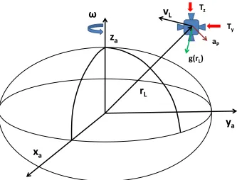
In formulating the spacecraft guidance problem for close-proximity operations around asteroids, we model the spacecraft dynamics near the asteroid using a two-body gravitational model (spacecraft has negligible mass). The equations of motion for the spacecraft in a uniformly rotating, asteroid-fixed Cartesian coordinate frame having the origin at the asteroid center of mass are written as follows:

𝒓𝐿̇ = 𝒗𝐿 (1)

𝒗𝐿̇ = 𝟐𝝎 × 𝒗𝐿+ 𝝎 × 𝝎 × 𝒓𝐿+ 𝒈(𝒓𝐿) + 𝒂𝐶𝑂𝑀𝑀+ 𝒑 (2)

Here, 𝒓_𝐿= [𝑥, 𝑦, 𝑧]𝑇is the position vector in the body-fixed rotating frame, 𝒗_𝐿= [𝑣_𝑥, 𝑣_𝑦, 𝑣_𝑧]𝑇is the velocity vector, 𝒈(𝒓𝐿) = [𝑔𝑥, 𝑔𝑦, 𝑔𝑧]𝑇is the local gravitational field, 𝒂𝐶𝑂𝑀𝑀= [𝑎𝑐𝑥, 𝑎𝑐𝑦, 𝑎𝑐𝑧]𝑇is the acceleration command and 𝒑 = [𝑝_𝑥, 𝑝_𝑦, 𝑝_𝑧]𝑇is the perturbing acceleration, accounting for unmodeled/unknown forces (e.g. gravity field inaccuracies, solar radiation pressure and nth-body perturbations).

For this analysis, it is assumed that the shape of the asteroid can modeled as a triaxial ellipsoid allowing analytical determination of the asteroid gravitational field. The gravitational field can be expressed as a partial derivative of the potential field, i.e. 𝒈(𝒓_𝑳) = 𝜕𝑉 𝜕𝒓⁄ _𝑳𝑇.

The equations of motion can be explicitly written in their scalar form:

𝑥̇ = 𝑣𝑥 (3)

𝑦̇ = 𝑣𝑦 (4)

𝑧̇ = 𝑣𝑧 (5)

𝑣̇𝑥= 2𝜔𝑣𝑦+ 𝜔2𝑥 +𝜕𝑉_𝜕𝑥+ 𝑎𝐶𝑥+ 𝑝𝑥 (6)

𝑣̇𝑦= −2𝜔𝑣𝑥+ 𝜔2𝑦 +𝜕𝑉_𝜕𝑦+ 𝑎𝐶𝑦+ 𝑝𝑦 (7)

𝑣̇𝑧=𝜕𝑉_𝜕𝑧+ 𝑎𝐶𝑧+ 𝑝𝑧 (8)

The mathematical model described in Eq. (1-8) is employed to derive the guidance equations. In the development of the guidance law, the mass of the spacecraft is assumed to be constant. However, in more realistic Monte Carlo simulations required to test the performance of the proposed OSG law, the model is upgraded to account for mass variation as given by the classical rocket equation:

𝑚̇ = −_𝐼‖𝑻‖

𝑠𝑝𝑔𝑐 (9)

B.Non-linear Guidance Algorithms Development

The goal of this paper is to present a set of targeting and real-time guidance algorithms for asteroid close-proximity operations. Such algorithms are designed by combining some known results from optimal control theory as applied to the landing problem10,12_{and advancements in non-linear sliding control theory}15_{. The sliding control} approach to targeting requires a geometric understanding of the control problem. The idea of using sliding control modes for real-time guidance is rooted into employing “surfaces” to drive the dynamical system to the desired state. A sliding surface is defined as a linear combination of the state error and/or its derivative. Whenever the system state (position and velocity) is locked on the sliding surface, the dynamical system is tracking the desired reference signal with null error.

Proper development of sliding-based guidance algorithms require the definition of a suitable guidance model which is presented next.

1. Guidance model: Zero-Effort Miss (ZEM) and Zero-Effort Velocity (ZEV) errors

The physical model employed to develop the guidance algorithm is a 3-DOF model similar to the one presented in the previous section (see Eq. (1)-(8)). However, the guidance model does not account for a mass variation. The equations can be synthetically represented as follows:

𝑑

𝑑𝑡𝒓𝐿= 𝒗𝐿 (10)

𝑑

𝑑𝑡𝒗𝑙= 𝒂𝐿(𝑡) = 𝒈(𝒓𝐿, 𝑡) + 𝒂𝐶𝑂𝑀𝑀(𝑡) (11) Here, the vector𝒈(𝒓𝐿, 𝑡) = 𝟐𝝎 × 𝒗𝐿+ 𝝎 × 𝝎 × 𝒓𝐿+ 𝜕𝑉 𝜕𝒓𝑳⁄ 𝑇 represents all forces acting on the spacecraft (except for the thrust) whereas aCOMM is the acceleration command (i.e. thrust-to-mass ratio) that drives the

z

_a

ω

r

_L

g(r

)

a

T

T

v

_L

x

_a

y

_a

spacecraft to the desired state. Eq. (10)-(11) can be integrated starting from knowledge of position and velocity at time t to formally determine position and velocity of the spacecraft at a specified final time tf:

𝒗𝐿(𝑡𝑓) = 𝒗𝐿(𝑡) + ∫ (𝒈(𝒓𝐿, 𝜏) + 𝒂𝐶𝑂𝑀𝑀_𝑡𝑡𝑓 (𝜏))𝑑𝜏 (12)

𝒓𝐿(𝑡𝑓) = 𝒓𝐿(𝑡) + 𝒗𝐿(𝑡)𝑡𝑔𝑜+ ∫ ∫ (𝒈(𝒓𝐿, 𝜏′) + 𝒂𝐶𝑂𝑀𝑀_ttf _𝜏′𝑡𝑓 (𝜏′))𝑑𝜏′𝑑𝜏 (13)

Here tgo = tf – t is the time-to-go, i.e. the time required to reach the desired position (target) with the desired velocity. Next, we define the following quantities:

Definition #1: Given the time t, we define the Zero-Effort Miss (ZEM) as the distance (vector) the spacecraft will miss the target if no acceleration command (guidance) is generated after t:

𝒁𝑬𝑴(𝑡) = 𝒓𝐿𝑓− 𝒓𝐿(𝑡𝑓), 𝒂𝐶𝑂𝑀𝑀(𝜏) = 𝟎, 𝜏 ∈ [𝑡, 𝑡𝑓] (14)

Definition #2: Given the time t, we define the Zero-Effort Velocity (ZEV) as the error in velocity at the final time, if no acceleration command (guidance) is generated after t, i.e.

𝒁𝑬𝑽(𝑡) = 𝒗𝐿𝑓− 𝒗𝐿(𝑡𝑓), 𝒂𝐶𝑂𝑀𝑀(𝜏) = 𝟎, 𝜏 ∈ [𝑡, 𝑡𝑓] (15)

Here, 𝒓𝐿𝑓and 𝒗𝐿𝑓 are the desired position and velocity at the final time. Both 𝒁𝑬𝑴(𝑡) and 𝒁𝑬𝑽(𝑡)can be explicitly expressed as functions of the current position, velocity and time-to-go by substituting Eq. (12, 13) with aCOMM= 0 into Eq.(14) and Eq.(15):

𝒁𝑬𝑽(𝑡) = 𝒗𝐿𝑓− 𝒗𝐿(𝑡) − ∫ 𝒈(𝒓𝐿, 𝜏)𝑑𝜏𝑡𝑓

𝑡 (16) (7)

𝒁𝑬𝑴(𝑡) = 𝒓𝐿𝑓− 𝒓𝐿(𝑡) − 𝒗𝐿(𝑡)𝑡𝑔𝑜− ∫ ∫ 𝒈(𝒓𝐿, 𝜏′)𝑑𝜏𝑡𝑓 ′_𝑑𝜏 𝜏′

t_f

t (17)

2. Optimal guidance for lunar landing: Basic equations

The basis of our algorithm development is the ability to generate an optimal guidance law as a function of 𝒁𝑬𝑴and 𝒁𝑬𝑽. Indeed, given the actual spacecraft position and velocity, both quantities can be estimated on-line by the numerical integration of the (unperturbed) equations of motion as functions of the time-to-go and the targeted conditions. One of the key ingredients is the ability to obtain a closed loop guidance law that minimizes the overall guidance effort, i.e. a guidance law thatminimizes the overall acceleration command. The problem can be formulated as follows:

Find the 𝒂𝐶𝑂𝑀𝑀 as a function of 𝒁𝑬𝑴(𝑡) and 𝒁𝑬𝑽(𝑡)that minimizes the following performance index: 𝐽(𝒂𝐶𝑂𝑀𝑀) = ∫ 𝒂𝐶𝑂𝑀𝑀(𝜏)𝑡𝑓 𝑇_{𝒂𝐶𝑂𝑀𝑀(𝜏)𝑑𝜏}

𝑡 (18)

Subject to Eq. (11, 12) as physical constraints, with initial conditions (at time t) r(t) and v(t) and final conditions (at time tf) rL and vL.

The acceleration command is assumed to be unconstrained, i.e. the thrust generated by the propulsion system is unbounded. The problem can be solved by either applying the Pontryagin Minimum Principle (PMP) to determine the necessary conditions for the existence of an optimal solution (Two-Point Boundary Value Problem, TPBVP) or by a direct application of calculus of variations (see appendix A). It is found that the acceleration command is linear in time, i.e.:

The constants A1 and A2 are determined by substituting aCOMM in Eq. (12)-(13). Finally, the optimal acceleration command can be expressed as a function of ZEM(t), ZEV(t) and tgo as follows:

𝒂𝐶𝑂𝑀𝑀(𝑡) =_𝑡𝑘𝑅

𝑔𝑜2 𝒁𝑬𝑴(𝑡) + 𝑘𝑉

𝑡_𝑔𝑜𝒁𝑬𝑽(𝑡) (20)

Where kR = 6, and kV = -2 are the optimal guidance gains (details of the derivation are presented in appendix A). The methodology employed to determine the optimal guidance law as a function of 𝒁𝑬𝑴and 𝒁𝑬𝑽 is very similar to the analysis presented by D’Souza13_{, who derived the optimal acceleration command for a power landing} descent as a function of error in position (actual position minus target position), velocity (actual velocity minus target velocity) and time-to-go. Both formulations do not impose any constraints in term of maximum thrust or minimum altitude. Nevertheless, both algorithms are easy to implement and mechanize which may justify the attractiveness of the guidance approach.Numerical simulations of the closed-loop trajectories may be analyzed a-posteriori to verify that both constraints are never violated or that the guidance algorithm works (i.e. guides the spacecraft to the target) even in the presence of thrust saturation.

3. Sliding Control Theory

The sliding control methodology is an elementary approach to robust control15_{. Intuitively, it is based on the} observation that it is much easier to control non-linear and uncertain 1st _{order systems (i.e. described by 1}st _order differential equations) than nth_{-order systems (i.e. described by n}th_{-order differential equations). Generally, if a} transformation is found such that an nth_{-order problem can be replaced by a 1}st _{order problem, it can be shown that,} for the transformed problem, perfect performance can be in principle achieved in presence of parameter inaccuracy. As a drawback, such performance is generally obtained at the price of higher control activity.

Consider the following single-input nth_{-order dynamical system:}

𝑑𝑛

𝑑𝑡𝑛𝑥 = 𝑓(𝒙) + 𝑏(𝒙)𝑢 (21)

Here, x is the scalar output, u is the control variable and 𝒙 = [𝑥, 𝑥̇, … . . , 𝑥(𝑛)]𝑻 is the state vector. Both 𝑓(𝒙), which describes the non-linear system dynamics, and the control gain 𝑏(𝒙) are not exactly known. Assuming that both 𝑓(𝒙) and 𝑏(𝒙) have a known upper bound, the sliding control goal is to get the state 𝒙 to track the desired state 𝒙𝒅= [𝑥𝑑, 𝑥̇𝑑, … . . , 𝑥_𝑑(𝑛)]𝑻 in presence of model uncertainties. The time varying sliding surface is introduced as a function of the tracking error 𝒙̃ = 𝒙 − 𝒙_𝒅 by the following scalar equation:

𝑠(𝒙, 𝑡) = (_𝑑𝑡𝑑+ 𝜆)𝑛−1_{𝒙̃ = 0 (22)}

For example, if n = 2 we obtain:

𝑠(𝒙, 𝑡) = 𝒙̃̇ + 𝜆𝒙̃ = 0 (23)

Importantly, λ is a strictly positive parameter. With the definitions in Eq. (22) and Eq. (23), the tracking problem is reduced to the problem of forcing the dynamical system in Eq. (21) to remain on the time-varying sliding surface. Clearly, tracking an n-dimensional vector 𝒙𝒅 has been reduced to the problem of keeping the scalar sliding surface to zero, i.e. the problem has been reduced to a 1st _{order stabilization problem in s. The simplified 1}st _order stabilization problem can be now achieved by selecting a control law such that outside the sliding surface the following is satisfied:

1 2 𝑑 𝑑𝑡𝑠

2_{≤ −𝜂|𝑠| (24)}

𝑉(𝑠) =1₂𝑠𝑇_{𝑠 (25)}

With 𝑉(0) = 0 and 𝑉(𝑠) > 0for 𝑠 > 0. By taking the derivative of Eq. (25), it is easily concluded that the sliding condition (Eq. (24)) is satisfied. The control law is generally obtained by substituting the sliding control definition, Eq. (23), and the system dynamical equations, Eq. (21), into Eq. (24).

C.Optimal Sliding Guidance (OSG) Design

The mathematical expression of the acceleration command is fairly simple and may be attractive for direct implementation on the on-board guidance computer. However, the optimal guidance, as derived, does not account for unmodeled disturbances which may negatively affect its performance. Here, the overall goal is to integrate a non-linear sliding control mode into the optimal guidance law to produce a robust, non-linear guidance algorithm.

To implement the sliding control approach into the optimal guidance framework and derive the Optimal Sliding Guidance (OSG) equations, we begin by defining a sliding surface (vector) as a function of ZEM and ZEV as follows:

𝒔 = 𝒁𝑬𝑽 + 𝜆̃𝒁𝑬𝑴 (26)

Clearly, the surface goes to the null value as ZEM and ZEV both approach zero. Subsequently, the idea is to construct the guidance law in such a way that the system is always driven to the sliding surface. Therefore, we consider the dynamics of the sliding surface, i.e. take the derivative of Eq.(21) and substitute the expressions for the derivative of ZEM and ZEV:

𝑑 𝑑𝑡𝒔 =

𝑑

𝑑𝑡𝒁𝑬𝑽 + 𝜆̃ 𝑑

𝑑𝑡𝒁𝑬𝑴 = −(1 + 𝜆̃𝑡𝑔𝑜)𝒂𝐶𝑂𝑀𝑀 (27)

If the optimal aCOMM,as derived above, is substituted into Eq.(28), we obtain:

𝑑

𝑑𝑡𝒔 = − [(1 + 𝜆̃𝑡𝑔𝑜) 𝑘𝑉

𝑡_𝑔𝑜𝒁𝑬𝑽 + (1 + 𝜆̃𝑡𝑔𝑜) 𝑘𝑅

𝑡_𝑔𝑜2 𝒁𝑬𝑴] = −𝐾(𝑡)(𝒁𝑬𝑽 + 𝜆̃𝒁𝑬𝑴) = −𝐾(𝑡)𝒔 (28) The following relationships between the parameters can be easily found:

𝐾(𝑡) = (1 + 𝜆̃𝑡𝑔𝑜)𝑘𝑉

𝑡_𝑔𝑜 (29)

𝜆̃𝐾(𝑡) = (1 + 𝜆̃𝑡𝑔𝑜)_𝑡𝑘𝑅

𝑔𝑜2 (30)

𝜆̃ = 𝑘𝑅

𝑘_𝑉𝑡_𝑔𝑜 (31)

The sliding surface behaves as a non-linear first order system and its dynamics depend explicitly on the time-to-go or 𝑡_𝐹− 𝑡. Consequently, the system has the properties to reach the surface in a finite time which occurs exactly when 𝑡𝐹= 𝑡 or at the landing point. Thus the surface is reached for the first time at the landing point and chattering is avoided (see Appendix B for a detailed analysis of the sliding surface dynamics). The sliding mode is incorporated into the optimal guidance law to guarantee that the sliding surface behaves as follows:

𝑑

𝑑𝑡𝒔 = −𝐾(𝑡)𝒔 − Φ

𝑡_𝑔𝑜𝑠𝑖𝑔𝑛(𝒔) (32)

𝒂𝐶𝑂𝑀𝑀(𝑡) = 𝑘𝑅

𝑡_𝑔𝑜2 𝒁𝑬𝑴(𝑡) + 𝑘_𝑉

𝑡_𝑔𝑜𝒁𝑬𝑽(𝑡) − Φ

𝑡_𝑔𝑜𝑠𝑖𝑔𝑛(𝒔) (33)

The Lyapunov’s second method is now employed to show that the OSG is globally stable and robust against perturbations. Consider the following quadratic function as a candidate Lyapunov function:

𝑉 =1₂𝑠𝑇_{𝑠 =}1

2(𝒁𝑬𝑽 + 𝜆̃𝒁𝑬𝑴) 𝑇

(𝒁𝑬𝑽 + 𝜆̃𝒁𝑬𝑴) (34)

Differentiating with respect to time, we obtain: 𝑑

𝑑𝑡𝑉 = 𝒔 𝑇 𝑑

𝑑𝑡𝒔 = 𝒔 𝑇₍𝑑

𝑑𝑡𝒁𝑬𝑽 + 𝑘𝑉 𝑘𝑅𝑡𝑔𝑜

𝑑

𝑑𝑡𝒁𝑬𝑴) (35)

Inserting the expressions for the derivative of ZEM and ZEV: 𝑑

𝑑𝑡𝑉 = 𝒔 𝑇 𝑑

𝑑𝑡𝒔 = 𝒔

𝑇_{(−𝒂𝐶𝑂𝑀𝑀+ 𝒑(𝑡) −}𝑘𝑅

𝑘_𝑉(𝒂𝐶𝑂𝑀𝑀− 𝒑(𝑡))) =

= 𝒔𝑇_{(− (}𝑘𝑅+𝑘𝑉

𝑘𝑉 ) 𝒂𝐶𝑂𝑀𝑀+ ( 𝑘_𝑅+𝑘_𝑉

𝑘𝑉 ) 𝒑(𝑡)) =

= 𝒔𝑇_{(− (}𝑘𝑅+𝑘𝑉 𝑘_𝑉 ) (

𝑘_𝑅

𝑡_𝑔𝑜2 𝒁𝑬𝑴(𝑡) + 𝑘_𝑉

𝑡_𝑔𝑜𝒁𝑬𝑽(𝑡) − Φ

𝑡_𝑔𝑜𝑠𝑖𝑔𝑛(𝒔)) + ( 𝑘_𝑅+𝑘_𝑉

𝑘_𝑉 ) 𝒑(𝑡)) =

= 𝒔𝑇_{(− (}𝑘𝑅+𝑘𝑉

𝑡𝑔𝑜 ) (𝒁𝑬𝑽(𝑡) + 𝑘_𝑅

𝑘𝑉𝑡𝑔𝑜𝒁𝑬𝑴(𝑡)) − ( 𝑘_𝑅+𝑘_𝑉

𝑘𝑅 ) (− Φ

𝑡𝑔𝑜𝑠𝑖𝑔𝑛(𝒔) + 𝒑(𝑡))) =

= (𝑘𝑅+𝑘𝑉 𝑡_𝑔𝑜 ) 𝒔

𝑇_{𝒔 + (}𝑘𝑅+𝑘𝑉 𝑘_𝑅 ) (−

Φ

𝑡_𝑔𝑜𝑠𝑖𝑔𝑛(𝒔) + 𝒑(𝑡)) (36)

Now, substituting kR = 6 and kV = -2 and assuming that Φ > ||p|| we get:

𝑑 𝑑𝑡𝑉 = −

4 𝑡_𝑔𝑜‖𝒔‖

2_{− 2𝒔}𝑇₍Φ

𝑡_𝑔𝑜𝑠𝑖𝑔𝑛(𝒔) + 𝒑(𝑡)) = − 2 𝑡_𝑔𝑜(2‖𝒔‖

2_{+ Φ𝒔}𝑇_{𝑠𝑖𝑔𝑛(𝒔) + 𝒔}𝑇_{𝒑(𝑡)) ≤ 0 (37)}

Therefore, Lyapunov function’s derivative is shown to be negative definite. Moreover, the selected Lyapunov function (Eq.(35) is definite positive and radially unbounded. Finally, 𝑉(𝒔) is shown to be decrescent (see Appendix C). All the above conditions ensure global stability for the proposed OSG (See Appendix C for a formal statement of the theorem).

III.

Guidance Implementation and Simulations

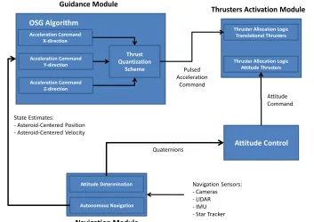
in Fig. 2, it is assumed that the guidance and attitude functions are independent. More specifically, it is assumed that the only function of the attitude module is to maintain the body-fixed spacecraft reference frame aligned with the asteroid-centered frame. In this case, the guidance algorithm can generate three independent acceleration commands along the asteroid fixed directions.

The thrust vector is then quantized and limited to create the commanded thrust

T

𝑻𝐶(𝑖) = {

𝑇𝑚𝑎𝑥 𝑖𝑓 𝑻𝐶(𝑖) > 𝑇𝑡ℎ𝑟𝑒𝑠ℎ𝑜𝑙𝑑 0 𝑖𝑓 𝑇𝑡ℎ𝑟𝑒𝑠ℎ𝑜𝑙𝑑< 𝑻𝐶(𝑖) < 𝑇𝑡ℎ𝑟𝑒𝑠ℎ𝑜𝑙𝑑 −𝑇𝑚𝑎𝑥 𝑖𝑓 𝑻𝐶(𝑖) < −𝑇𝑡ℎ𝑟𝑒𝑠ℎ𝑜𝑙𝑑

} 𝑓𝑜𝑟 𝑖 = 1,2,3 (38)

B. OSG Performance Analysis

The OSG algorithm is shown to theoretically guide the spacecraft to any desired state around the asteroid. The target state is defined as function of the close proximity operations required to accomplish a specific mission (e.g. landing, hovering). To fully test the ability of the algorithm to execute the assigned tasks, a realistic simulation environment describing the guided spacecraft dynamics around a selected asteroid of our choice is defined and implemented in MATLAB®. The simulation environment describes the 3-D spacecraft motion in an asteroid body-fixed reference frame (see Eq. (1)-(9)). Moreover, the following modeling assumptions have been considered:

1. The asteroid is assumed to wobble around its axis with a known nutation angle and spin rate.

2. The asteroid parameters (spin rate, nutation angle, density and dimensions) are assumed to be known.

3. The spacecraft thrusters have a response to the guidance signal described by a first order dynamicswith a known time constant.

4. Mass flow rate errors are statistical in nature and modeled with a uniform distribution.

5. Sensor errors are assumed to be described by a Gaussian distribution with a known standard deviation. Acceleration Command

Z-direction

Acceleration Command

Y-direction Acceleration Command

X-direction

Guidance Module

OSG Algorithm

Thrust Quantization

Scheme

Thruster Allocation Logic Translational Thrusters

Thruster Allocation Logic Attitude Thrusters

Autonomous Navigation Attitude Determination

Attitude Control

Thrusters Activation Module

State Estimates:

- Asteroid-Centered Position - Asteroid-Centered Velocity

Quaternions

Attitude Command Pulsed

Acceleration Command

Navigation Module

Navigation Sensors: - Cameras - LIDAR - IMU - Star Tracker

6. Gravity field is computed assuming the asteroid is described by a tri-axial ellipsoid of known dimensions. The known gravity field is perturbed by a Gaussian noise with a 10% standard deviation.

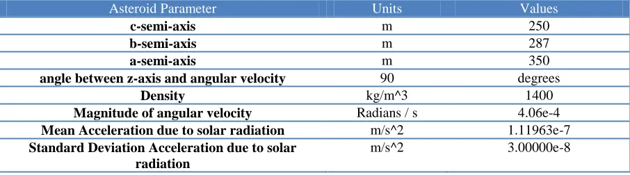
A set of Monte Carlo simulations have been executed to test the performance of the OGS algorithm in close-proximity operations scenarios typically planned during asteroid exploration missions. More specifically, we considered 1) a powered equatorial soft landing, where the spacecraft lands on a specified equatorial site of the selected asteroid and 2) a TAG maneuver, where the spacecraft touches the asteroid surface for a very short time. TAGs may be generally required to acquire an asteroid sample16_{.The guided maneuvers are assumed to be executed} white operating around 1999 RQ36 “Bennu”. Table 1 shows the nominal asteroid parameters describing the environment around Bennu. Table 2 shows the spacecraft parameters employed in the Monte Carlo simulations. Table 3 show the spacecraft initial conditions (the spacecraft is assumed to be in a terminator orbit) and final equatorial target state.

1. OSG AsteroidSoft Landing

In the first set of Monte Carlo tests for the OSG algorithm, we considered a scenario where the spacecraft executes a guided autonomous landing in the equatorial region of Bennu. The spacecraft is assumed to leave a nominal terminator orbit and autonomously employs OSG to navigate toward the desired state. A waypoint navigation approach is employed. More specifically, the spacecraft targets an initial state (waypoint) located at an intermediate position between the initial state and final target state. The OSG targets the waypoint first and, once achieved it within a specified tolerance switches to the final target as desired target. Table 4 shows the initial, intermediate waypoint and final state.

A set of 1000 Monte Carlo simulations has been executed to analyze the guidance performances. Importantly, the spacecraft’s mass is varied randomly between its nominal value and 10% less than this nominal value (uniform

Table 1: 1999 RQ36 “Bennu” Nominal parameters

Asteroid Parameter Units Values

c-semi-axis m 250

b-semi-axis m 287

a-semi-axis m 350

angle between z-axis and angular velocity 90 degrees

Density kg/m^3 1400

Magnitude of angular velocity Radians / s 4.06e-4

Mean Acceleration due to solar radiation m/s^2 1.11963e-7

Standard Deviation Acceleration due to solar radiation

m/s^2 3.00000e-8

Table 2: Spacecraft Nominal Parameters

Spacecraft Parameter Units Values

Mass Kg 750

Engine mass flow rate variation Kg/sec 10%

Engine actuator delay Sec 0.25

Estimation errors (position and velocity) meters , m/sec 5%

Table 3: Initial and Target States

Trajectory Parameter Units Values

Position where spacecraft leaves orbit m (1500, 0, 0) + U(-100,100) Velocity where spacecraft leaves orbit m/s (-0.04, -0.047, -0.079) +U(-0.02, 0.02)

Landing Position m (0, -287,0)

distribution). The asteroid’s nutation angle, density, and angular velocity are also varied +/- 10% from their nominal values (uniform distribution). The latter reflects possible modeling errors in the measurement of the asteroid’s dynamics. To further stress the proposed OSG algorithm we increased the mean and standard deviation of the acceleration due to solar radiation pressure to 0.0001 m/s2 _{and 0.00001 m/s}2 _{respectively. A statistical model that} accounts for navigation error have been considered (5% standard deviation, 1-sigma, see Table 2). The guidance algorithm has been implemented and pulsed with 10 Hz frequency.

Figure 3 shows the results of the OSG-guided Monte Carlo simulations, reporting 3-D trajectories, the landing error ellipse (1-sigma) and the statistics associated with the landing errors. OSG is shown to perform very well in spite of the uncertain environment. Position and velocity errors are shown to be extremely low, which is an indication of the ability of the guidance algorithm to drive the spacecraft to the desired target with pinpoint accuracy.

Table 4: Initial and Target States

Leave Orbit

Position (m) Velocity (m/s) Time of flight (s)

(1500, 0, 0) + U(-100,100) (-0.04, -0.047, -0.079) +U(-0.02, 0.02) 4000

First Waypoint

Position (m) Velocity (m/s) Time of flight (s)

(150, -350, 0) (0.05, 0.05, 0.0) 1000

Landing

Position (m) Velocity (m/s) Time of flight (s)

(0, -287, 0) (0, 0, 0) N/A

2. OSG for TAG Maneuvers

The second set of Monte Carlo simulations has been implemented to simulate an autonomous TAG maneuver similar to the one designed for the upcoming NASA OSIRIS REx asteroid sample return mission. Touch-And-Go (TAG) maneuvers have been specifically conceived to touch the asteroid surface for a very short time required to collect a sample via the acquisition mechanism. Importantly, the trajectory includes a final unpowered terminal descent necessary to minimize sample contamination. The OSIRIS REx Flight Dynamics Team designed a set of three open-loop maneuvers aiming at satisfying the currently projected landing error requirement (< 25 meters). The sequence includes a) an initial burn required to leave the terminator (parking) orbit, b) an intermediate burn (checkpoint) at 125m altitude that target a point approximately 30 meters above the desired site with a vertical (descent) velocity less than 10 cm/sec and c) a final burn (matchpoint) that matches the asteroid angular velocity and initiates the vertical descent toward the asteroid surface. Importantly, thrusters are activated after the sample acquisition to escape the asteroid surface. The TAG maneuver sequence is designed on the ground and command uploaded after careful testing in a comprehensive simulation environment. Nevertheless, a limited level of autonomy is implemented on-board16_{.Indeed, the on-board GNC LIDAR is activated for asteroid limb detection which} provides range-to-go information and altitude measurements. Range-to-go and one single altitude sample are fed to an algorithm that adjusts burn magnitude, direction and timing to reduce further the TAG error ellipse16_.

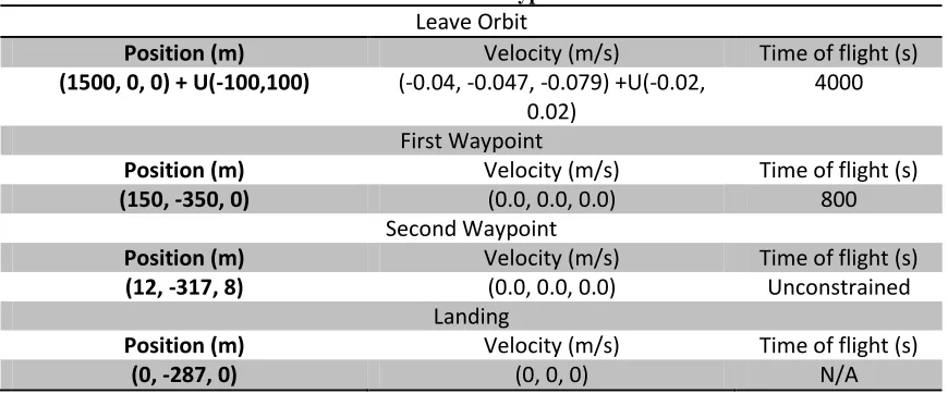
A similar a TAG maneuver scenario around Bennu has been implemented in our simulation environment to test the proposed guidance algorithm. In this case OSG is designed to target a set of two waypoints (checkpoint and matchpoint) defined to implement a TAG sequence for an equatorial landing. Table 5 shows the initial, intermediate and final target states. Importantly, the two intermediate waypoints have been designed such that the waypoint prior to the landing is located 30m above the intended sampling site. Once the 30m altitude is achieved, the spacecraft is allowed to fall toward the surface in an un-powered fashion. Note that the waypoint is selected to be not exactly above the desired landing point but somewhat offset to allow for drift caused by the asteroid’s rotation and the solar radiation pressure (estimated via modeling).

Table 5: TAG waypoints

Leave Orbit

Position (m)

Velocity (m/s)

Time of flight (s)

(1500, 0, 0) + U(-100,100)

(-0.04, -0.047, -0.079) +U(-0.02,

0.02)

4000

First Waypoint

Position (m)

Velocity (m/s)

Time of flight (s)

(150, -350, 0)

(0.0, 0.0, 0.0)

800

Second Waypoint

Position (m)

Velocity (m/s)

Time of flight (s)

(12, -317, 8)

(0.0, 0.0, 0.0)

Unconstrained

Landing

Position (m)

Velocity (m/s)

Time of flight (s)

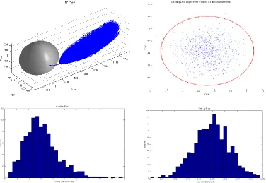
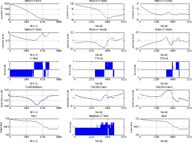
A set of 1000 Monte Carlo simulations has been executed to analyze the guidance performances. As in the precious case, the spacecraft’s mass is varied randomly between its nominal value and 10% less than this nominal value (uniform distribution). The asteroid’s nutation angle, density, and angular velocity are also varied +/- 10% from their nominal values (uniform distribution). The latter reflects possible modeling errors in the measurement of the asteroid’s dynamics. To further stress the proposed OSG algorithm we increased the mean and standard deviation of the acceleration due to solar radiation pressure to 0.0001 m/s2 _{and 0.00001 m/s}2 _{respectively. A statistical model that} accounts for navigation error have been considered (5% standard deviation, 1-sigma, see Table 2). The guidance algorithm has been implemented and pulsed with 1 Hz frequency. Figure 4 shows the 3-D Monte Carlo guided trajectories, the sampling error ellipse (1-sigma) and the histograms for the position and velocity errors. Table 6 reports details of the sampling error statistics. Figure 5 reports selected telemetry data for the case where the engine actuator delay time constant is 0s. This is equivalent to viewing the commanded thrust as opposite to the real thrust delayed by the time-response of the thruster.

The results indicate that the proposed OSG algorithm is capable of implementing pinpoint accuracy (<1m, 1-sigma) way beyond conventional open-loop TAG requirements.

Table 6: TAG sampling statistics

Figure 4. Monte Carlo simulations for the TAG maneuver. Top Left: 3-D guided trajectories. Top Right: TAG surface sampling spots and TAG error ellipse (1-sigma). Bottom Left: Histogram of the position error norm.

IV.

Conclusions and Future Efforts

In this paper, the theoretical development of a class of non-linear guidance algorithm for autonomous asteroid close-proximity operations has been discussed. The guidance design approach is based on a combination of optimal control theory and sliding control theory, yielding what has been named Optimal Sliding Guidance (OSG). Indeed, the generalized ZEM/ZEV feedback guidance is augmented by a sliding mode to ensure global stability. Importantly, the guidance law is naturally derived from the definition of an appropriate sliding surface that includes a combination of ZEM and ZEV. OSG has been tested in a set of realistic scenarios representing situations typically encounters in close-proximity operations around small bodies in general and asteroids in particular. The guidance algorithm is shown to perform well in a pulsed mode achieving pinpoint accuracy. Importantly, such class of algorithms may be functional to future mission where stringent sampling or landing requirements are required. Integration and testing of OSG with navigation algorithms (e.g. optical and LIDAR-based navigation) is currently underway.

V.

Appendix

A. Derivation of the ZEM/ZEV guidance law from Calculus of Variations

In this section, we apply optimal control theory to derive the optimal guidance equations (OGL, Eq. (21)). The optimal control problem can be formulated as follows:

Find the spacecraft acceleration command aCOMM(t) that minimizes the performance index J

𝐽 =1₂∫ 𝑎𝐶𝑂𝑀𝑀𝑇 _(𝜏)𝑎

𝐶𝑂𝑀𝑀(𝜏) 𝑡_𝑓

𝑡 (A1)

Subject to

{_{𝑣̇𝐿= 𝑎𝐿= 𝑔(𝑟𝐿, 𝑡) + 𝑎𝐶𝑂𝑀𝑀(𝑡)}𝒓̇𝐿= 𝒗𝐿 (A2)

With boundary conditions described as

{ 𝒓_𝐿(𝑡)=𝒓𝐿 𝒓𝐿(𝑡𝑓)=𝒓𝐿𝑓

𝒗_𝑳(𝑡)=𝒗𝐿 𝒗𝑳(𝑡𝑓)=𝒗𝐿𝑓

(A3)

Here, we apply calculus of variations to determine the necessary conditions for an extremal. Define the admissible functions as follows:

{

𝒓𝐿(𝑡, 𝛼) = 𝒓𝐿(𝑡) + 𝛼𝒉(𝑡) 𝒗𝐿(𝑡, 𝛼) = 𝒗𝐿(𝑡) + 𝛼𝒉̇(𝑡) 𝒂𝐿(𝑡, 𝛼) = 𝒂𝐶𝑂𝑀𝑀(𝑡) + 𝛼𝒉̈(𝑡)

(A4)

Where

{

𝒉(𝑡) = 𝒉(𝑡𝑓) = 𝟎 𝒉̇(𝑡) = 𝒉̇(𝑡𝑓) = 𝟎 𝒉̈(𝑡) = 𝒉̈(𝑡𝑓) = 𝟎

(A5)

The cost function is now a function of α

𝐽(𝛼) = 1₂∫ 𝒂𝐶𝑂𝑀𝑀𝑇 _(𝜏)𝒂

𝐶𝑂𝑀𝑀(𝜏)𝑑𝜏 𝑡_𝑓

𝑡 + 𝛼 ∫ 𝒂𝐶𝑂𝑀𝑀𝑇 (𝜏)𝒉̈(𝜏)𝑑𝜏 + 𝛼2

2 ∫ 𝒉̈

𝑇_{(𝜏)𝒉̈(𝜏)𝑑𝜏} 𝑡_𝑓

𝑡 𝑡_𝑓

𝑡 (A6)

The necessary condition for J(α) to be a minimum is written as 𝑑𝐽

𝑑𝛼|_𝛼=0= ∫ 𝒂𝐶𝑂𝑀𝑀

𝑇 _{(𝜏)𝒉̈(𝜏)𝑑𝜏 = 0} 𝑡𝑓

𝑡 (A7)

Integrating by parts twice we obtain: ∫ 𝒂𝐶𝑂𝑀𝑀𝑇 _{𝒂𝐶𝑂𝑀𝑀𝑑𝜏 = −}𝑑

𝑑𝑡𝒂𝐶𝑂𝑀𝑀

𝑇 _{(𝜏)𝒉̇(𝜏)|} 𝑡 𝑡_𝑓

+ ∫𝑡𝑓_𝑑𝜏𝑑2₂𝒂𝐶𝑂𝑀𝑀𝑇 _{(𝜏)𝒉(𝜏)𝑑𝜏} 𝑡

𝑡_𝑓

𝑡 = ∫

𝑑2

𝑑𝜏2𝒂𝐶𝑂𝑀𝑀𝑇 (𝜏)𝒉(𝜏)𝑑𝜏 𝑡_𝑓

𝑡 (A8)

Consequently:

𝑑𝐽

𝑑𝛼= 0 => ∫ 𝑑2

𝑑𝜏2𝒂𝐶𝑂𝑀𝑀𝑇 (𝜏)𝒉(𝜏)𝑑𝜏 = 0 𝑡_𝑓

𝑡 (A9)

We now use the fundamental lemma of calculus of variations 𝑑2

𝒗𝐿(𝑡) = 𝒗𝐿_𝑓− 𝑨₂1(𝑡𝑓+ 𝑡)𝑡𝑔𝑜+ 𝑨2𝑡𝑔𝑜+ ∫ 𝒈(𝒓𝐿, 𝜏)𝑑𝜏_𝑡𝑡𝑓 (A11)

𝒓𝐿(𝑡) = 𝒓𝐿𝑓− 𝒗𝐿(𝑡)𝑡𝑔𝑜− 𝑨1

6 (2𝑡 + 𝑡𝑓)𝑡𝑔𝑜 2 ₊𝑨2

2 𝑡𝑔𝑜

2 _{− ∫ ∫ 𝒈(𝒓}

𝐿, 𝜏′)𝑑𝜏′𝑑𝜏 𝑡_𝑓

𝜏′ t_f

t (A12)

Eq. (A11) and Eq. (A12) can be inverted to determine 𝑨1and 𝑨2. Remembering the definition of ZEM and ZEV (Eq. (17-18)) we have:

𝑨1= −_𝑡12 𝑔𝑜

3 (𝒁𝑬𝑴 − 1

2𝑡𝑔𝑜𝒁𝑬𝑽) (A13)

𝑨2= −_𝑡6

𝑔𝑜3 [(𝑡 + 𝑡𝑓)𝒁𝑬𝑴 − 1

3𝑡𝑔𝑜(2𝑡 + 𝑡𝑓)𝒁𝑬𝑽] (A14)

The OGL, i.e. the optimal acceleration command is determined by replacing Eq. (A13) and Eq. (A14) into Eq. (A10):

𝒂𝐶𝑂𝑀𝑀(𝑡) = − 12

𝑡𝑔𝑜3 (𝒁𝑬𝑴 − 1

2𝑡𝑔𝑜𝒁𝑬𝑽) 𝑡 + 6

𝑡𝑔𝑜3 [(𝑡 + 𝑡𝑓)𝒁𝑬𝑴 − 1

3𝑡𝑔𝑜(2𝑡 + 𝑡𝑓)𝒁𝑬𝑽] =

= −_𝑡2

𝑔𝑜𝒁𝑬𝑽 + 6

𝑡_𝑔𝑜2 𝒁𝑬𝑴 (A15)

Finally, setting 𝑘_𝑣= −2and 𝑘_𝑅= 6, we get: 𝒂𝐶𝑂𝑀𝑀(𝑡) = 𝑘𝑅

𝑡_𝑔𝑜2 𝒁𝑬𝑴(𝑡) + 𝑘_𝑣

𝑡𝑔𝑜𝒁𝑬𝑽(𝑡) (A16)

B. Sliding Surface Non-linear Dynamics

Consider a sliding surface with the following non-linear, first-order dynamics (see also Eq.(29)): 𝑑

𝑑𝑡𝒔 = −𝐾(𝑡)𝒔 = − 4 𝑡_𝑔𝑜𝒔 = −

4

𝑡_𝑔𝑜𝒔 (B1)

By using Eq.(29), Eq.(30) and Eq.(31) and remembering that kR = 6 and kV = -2, Eq.(B1) becomes an explicit function of the time-to-go or 𝑡_𝐹− 𝑡:

𝑑 𝑑𝑡𝒔 = −

4 𝑡𝑔𝑜𝒔 = −

4

𝑡𝐹−𝑡𝒔 (B2)

Here, we show that the system reaches the sliding surface in a finite time and exactly when 𝑡 = 𝑡_𝐹. Assume that the initial conditions are stated as (0) = 𝒔𝟎 . By applying the separation of variables we obtain:

𝑑𝑠_𝑖 𝑠_𝑖 = −

4𝑑𝑡

𝑡_𝐹−𝑡 (B3)

Where i = 1,2,3 are the components of the sliding surface vector. Eq.(B3) can be integrated to obtain:

𝑙𝑜𝑔(𝑠𝑖) = 4𝑙𝑜𝑔(𝑡𝐹− 𝑡) + 𝐶𝑖 (B4)

By imposing the initial conditions and taking the exponential of both sides, the solution becomes:

𝑠𝑖(𝑡) = 𝑠𝑖0(𝑡𝐹− 𝑡)4 (B5)

𝒔(𝑡) = 𝒔𝟎(𝑡𝐹− 𝑡)4 (B6)

𝒔̇(𝑡) = 4𝒔𝟎(𝑡𝐹− 𝑡)3 _(B7)

Eq.(B5)-(B7) are analytical expressions for the sliding surface vector and its derivative. Since the exponent of the RHS of both Eq.(B6) and Eq.(B7) is greater than zero, the surface will approach zero as 𝑡 → 𝑡𝐹 . More specifically, the surface is reached exactly when 𝑡 = 𝑡_𝐹 .

C. Global Stability Analysis of the OSG

ReferencesTo analyze the global stability of the proposed OSG algorithm, we rely on the following Lyapunov’s stability theorem [21]:

Uniform Global Asymptotic Stability for Non-Autonomous Systems: If in the whole state space, there exists a function 𝑉(𝒔, 𝑡) with continuous partial derivatives such that the following conditions are satisfied:

1. 𝑉(𝒔, 𝑡) is positive definite 2. 𝑉̇(𝒔, 𝑡) is negative definite 3. 𝑉(𝒔, 𝑡) is decrescent 4. 𝑉(𝒔, 𝑡) is radially bounded

Then the origin is uniformly globally asymptotically stable.(For the proof, see Slotine and Li [21] page 107). In our case, the system reaches the origin in a finite time 𝑡𝐹 and no switching (and consequently no chattering) is possible during the motion, i.e. the sliding surface is reached for the first time at the landing point (end of the flight). One of the key point is to show that the selected Lyapunov function (Eq.(34)) is decrescent. Using the analytical result obtained in Appendix B, it is possible to obtain an analytical expression for both the selected Lyapunov function and its derivative. Inserting Eq.(B6)-(B7) into Eq.(34) and Eq.(37) and ignoring the perturbations, we obtain:

𝑉 =1₂‖𝒔𝟎‖2(𝑡𝐹− 𝑡)8 (C1)

𝑉̇ = − 4 𝑡𝐹− 𝑡‖𝒔𝟎‖

2_(𝑡

𝐹− 𝑡)8— 2

𝑡𝐹− 𝑡Φ(|𝑠10| + |𝑠20| + |𝑠30|)(𝑡𝐹− 𝑡) 4₌

= −4‖𝒔𝟎‖2_(𝑡

𝐹− 𝑡)7— 2Φ(|𝑠10| + |𝑠20| + |𝑠30|)(𝑡𝐹− 𝑡)3 (C2)

The Lyapunov function is obviously decrescent with time and goes to zero as 𝑡 → 𝑡_𝐹 . However, the statement can be formally proven by finding a uniform function that bounds 𝑉̇ :

𝑉̇ = −4‖𝒔𝟎‖2_(𝑡

𝐹− 𝑡)7— 2Φ(|𝑠10| + |𝑠20| + |𝑠30|)(𝑡𝐹− 𝑡)3≤ −4‖𝒔𝟎‖2(𝑡𝐹− 𝑡)7 (C3)

The uniform global asymptotic stability follows with 𝑊(𝒔) = 4‖𝒔_𝟎‖2(𝑡_𝐹− 𝑡)7

VI.

References

1_{F. J. Ciesla, S. B. Charnley, The physics and chemistry of nebular evolution, in: Lauretta, D.S., McSween, H.Y. (Eds.),}

Meteorites and the Early Solar System II. University of Arizona Press, Tucson, pp.209–230, 2006.

2_{J. S. Kargel, Metalliferous asteroids as potential sources of precious metals, J. Geophys. Res. 99, (1994) pp. 21-129}

3_{National Research Council, Defending Planet Earth: Near-Earth Object Surveys and Hazard Mitigation Strategies, Final Report,}

4_{Lauretta, Dante et al., “An Overview of the OSIRIS-REx Asteroid Sample Return Mission” [#2491], 42th Lunar and Planetary}

Science Conference Abstracts, Lunar and Planetary Institute, Houston, Texas, 2012

5_{Lara, M., and Scheeres, D. J., “Stability Bounds for Three-Dimensional Motion Close to Asteroids,” Journal of the Astronautical}

Sciences, Vol. 50, No. 4, (2002), pp. 389–409.

6_{Miso, T., Tatsuaki Hashimoto, and KeikenNinomiya."Optical guidance for autonomous landing of spacecraft." Aerospace and}

Electronic Systems, IEEE Transactions on 35.2 (1999): 459-473.

7_{Shuang, Li, and Cui Pingyuan. "Landmark tracking based autonomous navigation schemes for landing spacecraft on asteroids."}

ActaAstronautica 62.6 (2008): 391-403.

8_{Bhaskaran, Shyam, et al. "Small Body Landings Using Autonomous Onboard Optical Navigation." The Journal of the}

Astronautical Sciences 58.3 (2011): 409-427.

9_{Furfaro, Roberto, Dario Cersosimo, and Daniel R. Wibben."Asteroid Precision Landing via Multiple Sliding Surfaces Guidance}

Techniques." Journal of Guidance, Control, and Dynamics (2013): 1-18.

10_{Levant, Arie. "Principles of 2-sliding mode design." Automatica 43.4 (2007): 576-586.}

11_{Guo, Yanning, Matt Hawkins, and Bong Wie."Applications of Generalized Zero-Effort-Miss/Zero-Effort-Velocity Feedback}

Guidance Algorithm." Journal of Guidance, Control, and Dynamics 36.3 (2013): 810-820.

12_{Battin, Richard H.An introduction to the mathematics and methods of astrodynamics.Aiaa, 1999.}

13_{D’Souza, Christopher N. "An optimal guidance law for planetary landing." Paper No. AIAA (1997): 97-3709.}

14_{Hawkins, Matt, YanningGuo, and Bong Wie. "ZEM/ZEV Feedback Guidance Application to Fuel-Efficient Orbital Maneuvers}

Around an Irregular-Shaped Asteroid." AIAA Guidance, Control, and Navigation Conference, Minneapolis, Minnesota. 2012.

15_{Slotine, Jean-Jacques E., and Weiping Li. Applied nonlinear control.Vol. 199.No. 1. New Jersey: Prentice hall, 1991.}