Data-driven adaptive model-based predictive control with application in wastewater systems

Wahab, Lisa and Katebi, Reza (2010) Data-driven adaptive model-based predictive control with application

to wastewater systems. IET Control Theory and Applications . ISSN 1751-8644

http://strathprints.strath.ac.uk/

27489

/

This is an author produced version of a paper published in

IET Control Theory and Applications .

ISSN 1751-8644

. This version has been peer-reviewed but does not include the final publisher proof

corrections, published layout or pagination.

Strathprints is designed to allow users to access the research output of the University of

Strathclyde. Copyright © and Moral Rights for the papers on this site are retained by the

individual authors and/or other copyright owners. You may not engage in further

distribution of the material for any profitmaking activities or any commercial gain. You

may freely distribute both the url (

http://strathprints.strath.ac.uk

) and the content of this

paper for research or study, educational, or not-for-profit purposes without prior

permission or charge. You may freely distribute the url (

http://strathprints.strath.ac.uk

)

of the Strathprints website.

Data-driven Adaptive Model-Based Predictive Control with

Application to Wastewater Systems

Journal: IET Control Theory & Applications Manuscript ID: CTA-2010-0068.R2

Manuscript Type: Regular Paper Date Submitted by the

Author: n/a

Complete List of Authors: Abdul Wahab, Norhaliza; Universiti Teknologi Malaysia, Electrical Engineering

Keyword: Adaptive Control, Model Predictive Control, Process Control, System Identification

[image:3.612.165.461.90.268.2]

Fig. 1: Comparison between direct and indirect methods

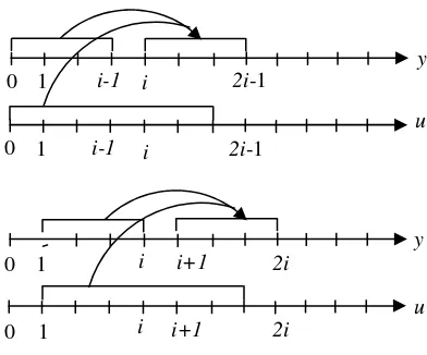
Fig. 2: Sliding window for i=4 y

u i-1 2i-1

y

u

0 1 i i+1 2i

0 1 i i+1 2i

0

0 1

1 i-1 _i i

2i-1

INPUT-OUTPUT DATA

System matrices (A,B,C,D) State estimate

Controller parameters

Direct method Indirect method

QR-

decomposition Least square

[image:3.612.196.392.359.522.2]

S, X, Q+Qr S, Xe, Q-Qw

S, Xr, Qr+Qw Settler Aerated

tank

Sin, Xin, Q

S, Xr, Qw

S, Xr, Qr

Fig. 3: Direct Adaptive Control

[image:4.612.169.445.102.235.2]

Fig. 4: Indirect Adaptive Control

Fig. 5: Activated Sludge Reactor MPC

design

Controller Plant

u y

uc

MPC parameters

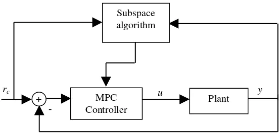
Subspace algorithm System

specification A,B,C,D,x0 MPC

Controller

Plant

u y

rc

Subspace algorithm

1200 1250 1300 1350 1400 40.8 41 41.2 41.4 41.6 S u b s tr a te ( m g /l )

1200 1250 1300 1350 1400

0.079 0.08 0.081 0.082 0.083 0.084 D ilu ti o n r a te ( 1 /h r)

1200 1250 1300 1350 1400

89 89.5 90 90.5 91 91.5 Time (hr) A ir f lo w r a te ( m 3 /h r)

1200 1250 1300 1350 1400

6.08 6.1 6.12 6.14 6.16 Time (hr) D O ( m g /l )

[image:5.612.111.499.77.375.2]

DAMBPC Ref IAMBPC

Fig. 6 : Performance comparison between DAMBPC and IAMBPC: set point tracking

Fig. 7: Performance comparison between DAMBPC and IAMBPC: disturbance rejection

1200 1250 1300 1350 1400

40.8 41 41.2 41.4 41.6 S u b s tr a te ( m g /l )

1200 1250 1300 1350 1400

0.079 0.08 0.081 0.082 0.083 0.084 D ilu ti o n r a te ( 1 /h r)

1200 1250 1300 1350 1400

6.08 6.1 6.12 6.14 6.16 Time (hr) D O ( m g /l )

1200 1250 1300 1350 1400

89 89.5 90 90.5 91 91.5 Time (hr) A ir f lo w r a te ( m 3 /h r)

[image:5.612.123.510.413.705.2]

1200 1250 1300 1350 1400 -1.5

-1 -0.5 0 0.5 1

1.5x 10

-3

∆

U

1

1200 1250 1300 1350 1400

-4 -2 0 2 4

Time (hr)

∆

U

2

DAMBPC IAMBPC

∆U1≤0.001

∆U2≤3

(a) Set point tracking

1200 1220 1240 1260 1280 1300 1320 1340 1360 1380 1400

-1.5 -1 -0.5 0 0.5 1 1.5x 10

-3

∆

U

1

1200 1220 1240 1260 1280 1300 1320 1340 1360 1380 1400

-4 -2 0 2 4

Time (hr)

∆

U

2

DAMPC IAMPC

∆U1≤0.001

∆U2≤3

DAMBPC IAMBPC

(b) Disturbance rejection

IET Control Theory & Applications

Data-driven Adaptive Model-Based Predictive Control with Application

to Wastewater Systems

Norhaliza A Wahaba*, Reza Katebib , Jonas Balderudc, M. Fuaad Rahmata

a _{Department of Control and Instrumentation Engineering, Faculty of Electrical Engineering, Universiti}

Teknologi Malaysia, Johor, Malaysia

b _{Industrial Control Centre, Dept of Electronic and Electrical Engineering, University of Strathclyde,}

Glasgow, UK

c_{Outokumpu Stainless AB, SE-693 81 Degerfors, Sweden}

Abstract: This paper is concerned with the development of a new data-driven adaptive model-based predictive controller (MBPC) with input constraints. The proposed methods employ subspace identification technique and a Singular Value Decomposition (SVD) based optimisation strategy to formulate the control algorithm and incorporate the input constraints. Both Direct Adaptive Model-Based Predictive Controller (DAMBPC) and Indirect Adaptive Model-Based Predictive Controller (IAMBPC) are considered. In DAMBPC, the direct identification of controller parameters is desired to reduce the design effort and computational load whilst the IAMBPC involves a two-stage process of model identification and controller design. The former method only requires a single QR decomposition for obtaining the controller parameters and uses a receding horizon approach to process input/output data for the identification. A suboptimal SVD-based optimisation technique is proposed to incorporate the input constraints. The proposed techniques are implemented and tested on a 4th order nonlinear model of a wastewater system. Simulation results are presented to compare the direct and indirect adaptive methods and to demonstrate the performance of the proposed algorithms.

Keywords: Activated sludge process, Adaptive control, Model-based predictive control, Subspace

2

1. Introduction

The classical control design problem is to start with building a model of the systems using physical laws to derive a presentation of the system in forms such as transfer function, matrix fraction, state space, impulse response, etc. While this approach works well for many systems, it has several disadvantages. The process of model building is expensive and cumbersome. Moreover, the models are valid only for a limited operating range and hence cannot capture the time varying or nonlinear behavior of many dynamic systems. As a consequence, many solution methods and algorithms were developed to design more effective controllers. The gain scheduling controllers were formally introduced in the sixties [1], followed by adaptive control approach in the seventies [2], neuro-fuzzy controllers in the eighties [2] and H-infinity robust control design in the nineties [3]. Most of these methods were however model-based and hence requires expensive effort to develop accurate models. Data driven methods use the process input/output data to design a stabilizing controller with satisfactory performance. This can include many of the adaptive control algorithms as well as neuro-fuzzy control design techniques. The data driven approach allows the controller to be designed using data from the actual system to be controlled under realistic operating conditions. Hence, the controller will stabilize the actual system instead of a model of that system. This procedure avoids the needs for modeling the plant under all hypothetical disturbances, and operating conditions, but considers only those that actually occur. A good background and application of data driven control are presented in [4] and [5], respectively.

This paper demonstrates the use of subspace-based techniques for the implementation of indirect and direct adaptive model-based predictive controller with input constraints. Subspace identification techniques have emerged as one of the more popular identification methods for the estimation of state space models. Using these techniques, subspace matrices, which obtained directly from input/output data, are used to obtain prediction of the process outputs. These predictions can subsequently serve as a basis for MBPC design. By continuously updating these predictions models, an adaptive predictive control method can be obtained. In IAMBPC, the controller is designed in two separate steps of model identification and control design. A more attractive alternative to the two-step method is to estimate the control parameters directly from the measurements (i.e. DAMBPC). The direct adaptive control method was developed in the early 70s

3

Some previous work has been reported on the design of MBPC using data driven control design method such as model-free Linear Quadratic Gaussian (LQG) and subspace predictive controller [7; 8; 9; 10], or controller designs using the state space model identified through subspace approach [11; 12]. It is shown in [7; 8] that the system identification and the calculation of controller parameters may be replaced by a single QR decomposition and hence a data driven controller can be formulated. Although the idea of combined subspace methods and MBPC as a data driven control design method has been around for few years, designing an adaptive subspace-based MBPC is still an open area of research. Existing methods in subspace- based adaptive MBPC does not include constraints [10], and hence one of the main attraction of predictive control design technique is missing from these methods. Therefore, the objective of this paper is to develop subspace based adaptive MBPC, which includes input constraints, as well as soft nonlinear dynamics. Wang et al. [14] have also employed similar approach but their work differs in term of the identification approach for the design of subspace controller, (e.g. the prediction of the future outputs presented by the past available measurements and past input signals.). Moreover, this paper highlights the advantage of using a suboptimal SVD-based optimisation technique to incorporate the input constraints as compared to QP method. Other approaches for dealing with these types of processes include nonlinear MBPC [13] and neural network based MBPC approaches [14]. The latter method has made few inroads in practice due to its complexity and computational load typically associated with these methods. For industrial applications, however, multiple model linear MBPC approaches tend to be more favoured [15; 16].

The proposed direct adaptive MBPC method can offer an attractive alternative to existing methods for slowly time-varying and nonlinear systems. The method combines the simplicity of linear MBPC with the power of a self-tuning controller to incorporate the hard input constraints. The main advantages are that the usually tedious and time-consuming modelling task can be relaxed and the controller can adapt to changing process conditions while the physical constraints are satisfied. The use of an SVD based method for optimisation reduces the computation burden and ensures that a solution can be found in a desired sampling time. The performance of DAMBPC is compared with IAMBPC using a 4th order nonlinear model of a wastewater system. Simulation results are presented to investigate the effect of prediction horizon on the tracking and disturbance rejection properties of the proposed algorithms.

4

simulation results where the performances of the proposed control strategies are compared. The paper ends with some conclusion.

2. The subspace identification method

A linear discrete time-invariant state space system can be represented as:

( 1) ( ) ( ) ( )

x k+ =Ax k +Bu k +Kv k (1)

( ) ( ) ( ) ( )

y k =Cx k +Du k +v k (2)

where u k( ), y k ( ) and x k( ) are the inputs, outputs and states respectively and ( )v k is a white noise

sequence with zero-mean and variance E v v[ p qT]=S

δ

pq. A B C D, , , and K are system matrices with

appropriate dimensions. We assume that

(

A B,

)

is controllable and

(

C A,

)

is observable. The following

matrix input-output equations [17] play an important role in the problem treated in linear subspace identification and it can be obtained by recursive substitution of Eq. (1) into Eq. (2):

f i f i f

Y = ΓX +H U and/or Yp = ΓiXp+H Ui p (3)

where the data block Hankel matrices for ( )u k represented as Upand Uf defined as:

              = − + − − 2 1 2 1 1 1 0 j i i i j j p u u u u u u u u u U L M O M M L L (4)               = − + − + + + − + + 2 2 2 1 2 2 1 1 1 j i i i j i i i j i i i f u u u u u u u u u U L M O M M L L (5)

The subscripts p and f represent ‘past’ and ‘future’ time. The outputs block Hankel matrices Yp and Yf

can also be defined in the same way. i is the prediction horizon (or so called Hp). Then, the data set is

broken into j prediction problem. The following shorthand notation is used for the past input-output data:

p p p U W Y   = _ _

  (6)

The future state sequence is defined as:

(

1 1

)

T

f i i i j

X = x x₊ K x_{+ −} (7)

5

1 i i C CA CA−      

Γ =  

      M , 1 2 0 0 0 i i i CB CAB CB H

CA B− CA− B CB

      =_{ }       L L

M M O M

L

(8)

The basic idea of subspace identification method is that, from the previously defined matrix

input-output Eq. (3), it can be observed that the block data Hankel matrix containing the future input-outputs, Yf is

linearly related to the future state sequences, Xi and the future inputs, Uf. Therefore, the main framework

of subspace model identification is to recover the termΓiXf , whereby from the knowledge of either Γi or

f

X , the state space system matrices can be retrieved in a least square sense [18]. Once the system

parameters are obtained, they can be used to design the controller.

This identification method is implemented for IAMBPC where the state space system matrices are

obtained using online subspace identification algorithm, i.e. Numerical algorithms for Subspace State Space

System IDentification (N4SID). For the DAMBPC controller parameters (subspace matrices) are directly

derived from the input-output measurement. The difference between two approaches is schematically shown

in Fig. 1. The following derivation is focused only for identifying the subspace matrices for the DAMBPC

method. The detail derivation on the subspace identification and the use of projection in subspace

identification are not presented here. They can be found in [18].

In the case when no noise is present, the actual future output Y_f lies in the combined row space

and the linear predictor equation can be written as:

ˆ

f w p u f

Y =L W +L U (9)

where W_p and U_f are the past inputs and outputs and future inputs, respectively. L_w and L_u are subspace

matrices corresponding to the states and inputs, respectively. By solving the following least square problem,

the output prediction, ˆYf can be extracted:

(

)

2 , , min F f p u w f Lu Lw U W L L

Y _

     

− (10)

The orthogonal projection of the row space of Yf into the row space spanned by Wpand Uf applied in Eq.

6

ˆ p f f f W Y Y U   = _ _

  (11)

ˆ _{/ /}

f

u f w p

f f U p f Wp f

L U L W

Y =Y W +Y U

14243

14243 (12)

from which we have two projections involved in the right hand side in the above equations. The first

projection of /

f

f U p

Y W relates to Kalman filter state of the system and the second projection of

/

p

f W f

Y U relates to Toeplitz matrix. Now, Eq. (12) can be solved efficiently via QR decomposition:

11 1

21 22 2

31 32 33 3

0 0 0 T p T f T f

W R Q

U R R Q

Y R R R Q

          ₌            _{  }     (13) By posing:

(

)

† 11 31 32 21 22 0 R

L R R

R R

 

= _{ }

  (14)

where L=

(

Lw Lu

)

and † denotes the Penrose-Moore pseudo inverse, Eq. (12) can be written as:

ˆ p p

f f

f f

W W

Y Y L

U U

   

= _{ }= _{ }

    (15)

where Lw and Luin Eq. (12) can be obtained by partitioning Lin Eq. (15):

[

]

p

w u f

f

W

L L Y

U

+

 

= _{ }

  (16)

[

]

1

p

T T T T

w u f p f p f

f

W

L L Y W U W U

U −        = _{ }_  _{ }_     (17)

where Nuand Ny denote the number of input and output, respectively. It can be observed that, the

subspace matrices L_w and L_ucan be retrieved directly from matrix R. The system matrices A, B, C, D

do not have to be calculated explicitly. To enable an adaptive sliding window, QR-updating is

performed. A combination of updating and down dating the QR decomposition is performed making

use of the rank-one modification [19]. The subspace matrices are updated online throughout the

updated R factor from the implemented QR updating.

As mentioned previously, the most interesting part in subspace model identification is that we can

7

parameters. The link between Kalman filtering and the projection of the future outputs Y_f into the

combined row space of the past inputs and outputs W_p and the future inputs U_f is demonstrated in Eq.

(12). We can now exploit the duality between Kalman filter and MBPC controller. For ,i j→ ∞, we

obtain:

ˆ /

f

f U p w p i f

Y W =L W = ΓX (18)

u i

L =H (19)

In general, L_w correspond to the determination of Kalman filter state and L_u represents the controller

parameters. It can be seen that there is a link between subspace projection and the Kalman filter

estimates, ˆXf of the state sequence Xf given by Eq. (18). When Lw is approximated to a lower order

matrix using singular value decomposition, it would be a rank deficient matrix of order n if there were

no noise. This description gives 1 1 1

T w

L ≈UΣV . Therefore, for 1/ 2 1 1

i U

Γ ≈ Σ and ˆ 1/ 21 1

T

f p

X ≈ Σ V W :

1/ 2 1/ 2 1 1 1 1

1 1 1

ˆ _. T

i f p

T p

w p

X U V W

U V W

L W

Γ = Σ Σ

= Σ

=

(20)

where Xˆf =xˆ1 is the steady state Kalman filter estimate and Γi is the extended observability matrix.

To obtain offset-free tracking, an integral action is included. Previous works that include integrator in the design of subspace controller are given in [9; 11]. The matrix input-output in Eq. (3) can be changed to include an integrator in the predictor and this can be expressed as follows:

f i f i f

Y S H U

∆ = Γ% + % ∆ ₍₂₁₎

ˆ

f i f i f

Y S H U

∆ = Γ% + % ∆ ₍₂₂₎

and ˆ

f w p u f

Y L W L U

∆ = % ∆ + ∆% ₍₂₃₎

where L%wand L%u are obtained directly from the previous identification of Lw and Lu. Thus:

ˆ

f t w p u f

Y =Y +L% ∆W + ∆L% U (24)

8

[

]

T

t t t t

Y = y y L y (25)

It should be noted that in any closed-loop parameter identification scheme, the input signal should be persistently exciting to perturb the main dynamics of the system. This can be usually achieved by injecting a Pseudo Random Binary Sequence Signal (PRBS) at the process set points. In practice for adaptive control algorithm, a degree of perturbation and excitation are also achieved during the identification and control design as the controller parameters changes as the control design is updated.

3. Adaptive Model-Based Predictive Control

The adaptive control scheme investigated here uses subspace identification technique described above. The measured data is collected over a sliding (receding) window. The procedure of using a sliding window for identification is illustrated in Fig. 2. Note that, data window used to identify subspace predictor parameters

should be expressed in term of future inputs uf =

(

ui−₁ K u₂i−₂

)

Tand measurement (past) inputs

(

0 1

)

T

p i

u = u K u₋ and outputs

(

0 1

)

T

p i

y = y K y₋ as described in Eq. (9). Here, the two prediction

problems should be solved at current time instant i and i+1 as shown in Fig. 2. The first prediction problem

(t=i) represents the case for obtaining the optimal prediction of i future outputs yˆ_f =

(

yˆ_i K yˆ_2i−1

)

Tusing

the information given in the previously stated data window up, yp and uf. The second prediction problem shows that the time instant slides (t=i to t=i+1) and similar meaning can be observed, only difference is the data window (up, yp and uf), which is, now slides from left to right. At every time step, for the new input-output data obtained, the subspace predictor parameters are updated online and the new control action is computed. Note that, the linear predictor in Eq. (24) is directly driven by input-output data and contains an integral action. The main advantage of this approach is that the controller parameters are updated at each sample time, which usually means a quicker response to process changes. The main drawback of this method is that a QR-decomposition needs to be computed at each sample instance, which increases the computation load.

9

performance index is exploited using SVD analysis within the context of subspace adaptive frameworks. We Two methods of subspace adaptive control scheme (DAMBPC and IAMBPC) are developed for the constrained case using SVD analysis

3.1. Direct method (DAMBPC)

A possible structure for direct adaptive control using MBPC is depicted in Fig. 3. To implement the DAMBPC, consider the linear predictor equation given in Eq. (24):

ˆ_{f w p u f}

y =L w% +L% ∆u (26)

The following MBPC performance index is minimised to calculate the control input increment, ∆u_f :

(

)

(

)

(

)

(

(

)

(

)

)

(

)

(

)

(

) (

)

1

1 0

ˆ ˆ

p c

H H

T T

i i

T _T

f f f f f f

J r k i y k i Q r k i y k i u k i R u k i

r y Q r y u R u

−

= =

= + − + + − + + ∆ + ∆ +

= − − + ∆ ∆

∑

∑

(27)

where Hpand Hcdenote the prediction horizon and control horizon, respectively. The output and input

weighting matrices are

Q=diag(Q1L QHp)>0 and R=diag(R1L RHc −1)≥0. Substituting Eq. (26) into Eq. (27) gives:

(

) (

T

)

_T

f w p u f f w p u f f f

J = r −L w% −L% ∆u Q r −L w% −L% ∆u + ∆u R u∆ (28)

where rf −L w%w p =e is the tracking error, thus:

2

T T T T

f u f f

J=e Qe− ∆u L Qe% + ∆ Ω∆u u (29)

where T H Nc u H Nc u

u u

L QL R ×

Ω = % + ∈_{R . To find the minimum of J, its derivative is set to zero:}

0

f

J u

∂ ₌

∂∆ (30)

The DAMBPC control law is therefore defined as:

1 T

f u

u

−

L Qe

∆

= Ω

%

₍₃₁₎

Eq. (31) gives the unconstrained optimal solution and the controller parameter L%_u is directly obtained from

10

The implementation of SVD based optimisation for the constrained case is discussed next. This makes the adaptive control scheme considerably faster and easier to implement as compared to QP method, since the Hessian Ω can be formed directly from the identification step. At each sampling instant, a feasible control sequence is determined by selecting a variable subset of the SVD basis representation. This sequence defined as ∆u satisfies the gain and rate input constraints of the optimisation problem (Eq. (29)) defined as

min max

( ) ( ) ( )

u k ≤u k ≤u k and ∆u k( )min ≤ ∆u k( )≤ ∆u k( )max.

To calculate the control input, let the SVD of Ωbe defined as [18]:

T T T

U V U U V V

Ω = Σ = Σ = Σ (32)

where Σ∈ H Nc u×H Nc u _{is given as:}

1

2

0 0

0 0

0 0

c u

H N σ

σ

σ

 

 

 

Σ =  

 

 

 

K K

M M O M

K

(33)

and σ1≥σ2≥K≥σH Nc u ≥0. The σi are the singular values of Σ and the vectors ui and vi are the

th

i

left singular vector and the ith right singular vector, respectively. In this case, since Ω is symmetric, the left

and right singular vectors are identical. This in turn, yields an important property that is the singular vector

matrix V is orthogonal i.e.

c u

T T

H N

V V=VV =I . If

(

₁, ,

)

c u

H N

V = v K v is orthogonal, then the vi form an

orthonormal basis vector for H Nc u

. Therefore, the following control input increment vectors:

(

( ) ( 1) ( _c 1)

)

T

u u k u k u k H

∆ = ∆ ∆ + K ∆ + − (34)

can be expressed as a linear combination of the singular vectors, v_i of Ωgiven as:

1

c u

H N

i i

i

u V u v u

=

∆ = ∆ =%

∑

∆% (35)

where vi =

(

v1, K, vH Nc u

)

are the columns of V, and ∆u%iare the entries of the input increment vector ∆u%.

The performance index, J, can now be written in terms of the new increment input vectors as:

2

T T T T T

u

J=e Qe− ∆u V L Qe% % + ∆ Σ∆u% u% (36)

This gives the optimal unconstrained control input increment sequence:

1 T T

uc u

u −V L Qe

11

The increment input vectors for the constrained case can be constructed by considering the modification of

the unconstrained solution, ∆u%uc in Eq. (37). Let us first define the performance index, J as:

(

,

)

2

1

min

c u

H N

uc i i uc i

u

i

J J σ u u

∆

=

= +

∑

∆ − ∆% % (38)

where ∆u%_{uc i,} is the ith entry of vector ∆u%_uc. From Eq. (38), it can be observed that whenever ∆ = ∆u%_i u%_{uc i,} ,

we obtain J=J_uc, which is the unconstrained value. Note that the entries of ∆u in Eq. (38) are arranged in

decreasing order of magnitude, sinceσ1≥σ2≥K≥σH Nc u ≥0, which starting from the one that influences

the performance index the most and ending with the one that influences the performance index the least. Therefore, to find a feasible solution to the constrained optimisation problem J, we need to consider

the components in the entries of vector ∆u%ucwith highest contribution in reducing the magnitude of J, i.e.

use those elements of ∆u%_uc with the biggest singular values. ∆u%_ucfor the unconstrained solution is:

, 1

c u

H N

uc uc i uc i

i

u V u v u

=

∆ = ∆% =

∑

∆% (39)

The vector ∆u%ucin Eq. (37) will be ordered from the highest to the smallest singular values and progressively

discarding smaller components, until the constraints are satisfied, i.e.:

(

1, , 0 0

)

T

uc uc m uc

u V u u

∆ = ∆% K ∆% K (40)

where

{

1

}

c u

H N c u

m∈I K H N . This does not necessarily gives the best control performance, hence the

following control increment vector is defined:

(

)

, 1 1,

1

m

svd i i uc m m uc

i

u v u v ₊α u ₊

=

∆ =

∑

∆% + ∆% (41)

where 0≤ ≤

α

1 and

{

1

}

c u

H N c u

m∈I K H N . To obtain the best solution

α

should be as large as

possible while the constraints are satisfied. For m=H N_{c u},

α

=0and the solution is unconstrained. The

proposed SVD-based DAMBPC is summarised here:

Algorithm 3.1 (Direct method)

Step 1: Construct data block Hankel matrix, i.e. Uf, Up, Yp, Yf from a given input-output data.

Step 2: Compute L by using Eq. (14), then partitioning L into L_w and L_u using Eqs. (16) and (17).

Step 3: Compute unconstrained solution, i.e. uuc 1V L QeT uT

−

∆_% = Σ %

12

(

1, , 1, 0 0

)

T

svd svd uc m uc m uc

u V u V u u α u ₊

∆ = ∆% = ∆% K ∆% ∆% K

lies on the boundary of the constraint set in H Nc u _and

svd

u

∆ ∈ ∆ . The parameters

m

and

α

are tuned

for the best performance whilst the constraints are satisfied

Step 5: At time k, only ∆u_svd(1) is implemented and the calculation is repeated at each time instant, i.e.

( )

u k is implemented as: ( )u k =u k( − + ∆1) u k( )

Step 6: Update the Hankel matrix using the newest data and go to step 2 and repeat.

3.2. Indirect method (IAMBPC)

For IAMBPC, the classical two-step of system identification and control design is performed. Firstly, a suitable model is estimated using subspace algorithm and then the controller parameters are calculated from a design method as shown in Fig. 4. The Numerical Algorithm for Subspace State Space System IDentification (N4SID) [20] is employed here for process identification.

By iterating the model in Eq. (1) - (2), the prediction output is defined as: ˆ_f

y = Γ + ∆x H u (42)

The quadratic performance index can be expressed as follows:

2

T T T T

J=e Qe− ∆u H Qe+ ∆u ∆u (43)

where =_{H QH}T + ∈_R H Nc u×H Nc u _and

f

e=r − Γx. The IAMBPC control law can be found by making the

gradient of J zero, therefore:

1 T

u −H Qe

∆ = (44)

By using SVD-based strategy, the performance index, J can now be rewritten as:

2

T T T T T

J=e Qe− ∆u V H Qe% + ∆ Σ∆u% u% (45)

Thus, the unconstrained optimal ∆uis:

1

u T T

uc V H Qe

−

∆% = Σ (46)

The derivation of the constrained solution using SVD-based optimisation strategy is similar to the one described in Section 3.1 and it is not repeated here. The IAMBPC algorithm is summarised here.

Algorithm 3.2: Indirect method

Step 1: Construct data block Hankel matrix, i.e. Uf, Up, Yp, Yf from a given input-output data.

13

Step 3: Compute the optimal unconstrained solution 1 T T uc

u −V H Qe

∆% = Σ

Step 4 – 6: Similar to Algorithm 3.1

4. Control of Activated Sludge Processes (ACT)

In this study, the proposed methods are applied to control a nonlinear activated sludge wastewater treatment plant. This process comprises an aerated tank and a settler as shown in Fig. 5. The bioreactor includes a secondary clarifier that serves to retain the biomass in the system while producing a high quality effluent. Part of the settled biomass is recycled to allow the right concentration of microorganisms in the aerated tank. A component mass balance that yields the following set of nonlinear differential equations was used [22]:

X t&( )=

µ

( ) ( )t X t −D t( )(1+r X t) ( )+rD t X t( ) _r( ) (47) ( ) ( ) ( ) ( )(1 ) ( ) ( ) in

t

S t X t D t r S t D t S

Y µ

= − − + +

& ₍₄₈₎

( ) o ( ) ( ) ( )(1 ) ( ) ( ( ) ( ) )

La s in

K t X t

C t D t r C t K C C t D t C

Y µ

= − + + − +

(49)

( ) ( ).(1 ). ( ) ( ).( ) ( )

r r

X t& =D t +r X t −D t

β

+r X t (50)

where the state variables, X(t), S(t), C(t) and Xr(t) represent the concentrations of biomass, substrate, dissolved oxygen (DO) and recycled biomass respectively. D(t) is the dilution rate, while Sin and Cin correspond to the substrate and DO concentrations of influent stream. The parameters r and β represent the ratio of recycled and waste flow to the influent flow rate, respectively. The kinetics of the cell mass production is defined in terms of the specific growth rate µ and the yield of cell mass Y. The term Ko is a constant. Cs and KLa denote the maximum DO concentration and the oxygen mass transfer coefficient, respectively. The quantity (W) appears in Eq. (49) through the oxygen transfer rate coefficient KLa:

La

K =ρW (51)

where

ρ

>0. The Monod equation gives the growth rate related to the maximum growth rate, to the

substrate concentration, and to DO concentration:

max

( ) ( ) ( )

( ) ( )

s c

S t C t

t

K S t K C t

µ =µ

+ + (52)

14

An adaptive control design scheme is required for this process as the dynamic is nonlinear and time varying. This is usually caused by the variation in the concentration and composition of the influent to the plant as well as 24-hrs changes in the influent flow. The process exhibits different dynamic under varying weather of dry, rain or storm conditions as well as variation in the daily temperature.

5. Evaluation and simulation results

Simulations were carried out for the two proposed control strategies that is, DAMBPC and IAMBPC methods. Both control methods use sliding identification window to update the parameters. The objective of the control algorithm is to regulate the substrate and DO concentrations from a steady state operating point at outputs 41.23 mg/l and 6.11 mg/l, respectively. For a fair comparison of both methods, the

horizons are set to H_p =20 and H_c=5. The weighting matrices were chosen as Q=diag 1,10

(

)

and

(

4 4

)

diag 10 ,10

R= − . The length of window is set to n=400. The constraints on the input change were

allowed to be ∆U1 ≤0.001and ∆U2 ≤3.0 .

Fig. 6 compares the set point tracking performance of the two control strategies. It can be seen that both methods exhibit similar response to set point changes as expected but the first control strategy has a slight overshoot. To be able to see that the controller achieves good disturbance rejection, the measurements of substrate and DO are corrupted with step input disturbance (Amp=0.01) at t=1285 and the performance of both design methods are compared as shown in Fig. 7.

It can be clearly seen that the DAMBPC design method is able to track back to the set point quickly. The controller also rejects the disturbance in a reasonable time. The IAMBPC design method takes longer to reach the set point. This is also evident from large peak in the first output signals (Substrate) before it is slowly track back to the set point. The control signals are also given as shown in Fig. 8. Both control methods can handle constraint effectively, as shown in Fig. 8.

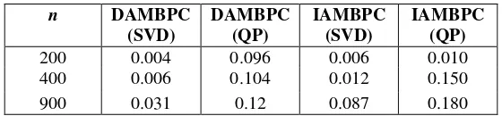
15

controller parameters, the summary of computation times (in sec) per sampling instant for different n and Hp for both methods is presented in Table 1 and Table 2, respectively. It can be clearly seen that the computation time required for SVD-based strategy is much lower (10 to 15 times) than the QP method. The SVD-based method shows an excellent performance, both for varying n and Hp. The tables also show the DAMBPC is faster than IAMBPC as expected.

5.1 Closed-loop Stability

The closed-loop stability of the proposed methods was extensively tested using simulation studies. The critical parameter to ensure the local stability when a local linear model is identified is the prediction horizon, Hp, and hence this must be selected carefully. Longer Hp will lead to better stability but this will also increase the computation load, and hence a trade-off should be made. Using the size of overshoot as an indication of stability, simulation results presented in Figs. 6 to 8 demonstrates that the DAMBPC has better stability robustness is than IAMBPC.

The overall closed-loop loop stability should also be analyzed for the nonlinear plant as stable linear local controllers are designed at each new operating condition. For the nonlinear process studied here, no global instability was observed as the system can in practice be stabilized by a set of PID controllers. Assuming the nonlinear plant is piecewise controllable and observable, the local MBPC controllers can then be designed to stabilize the nonlinear plant locally by choosing appropriate values for Hp. This does not, however, guarantee the global stability of the nonlinear plant. Johansson [23] shows that piecewise quadratic Lyapunov can be used for rigorous stability analysis of smooth nonlinear systems as well as quadratic stabilization of piecewise linear systems. The application of these techniques to the current problem is however out of scope of this paper.

6. Conclusions

The SVD- based data driven direct and indirect adaptive MBPC with input constraints were developed and tested in this paper. The derivation of DAMBPC control law only requires calculation of the subspace matrices Luand Lw. There is no need for explicit calculation of system matrices A, B, C, D. The

16

better tracking properties as well as disturbance rejection when applied to a nonlinear process. On the other hand, the use of SVD-based strategy in the optimisation structure significantly reduces the online computational time associated with the solution of standard QP method. In this case, the DAMBPC outperform the IAMBPC and it can provide an attractive alternative. For fast dynamical systems such as aircraft or vehicle dynamics, it may still be necessary to develop a version of these algorithms that uses the recursive subspace model identification such as R4SID.

Acknowledgments: The first author is supported financially by Malaysian Government and Universiti Teknologi Malaysia. This support is gratefully acknowledged.

References

[1] Leith _{D. J.} and W. E. Leithead: _{‘Survey of gain-scheduling analysis and design’, Int. J. Control, 2000,} Vol. 73, No. 11, pp. 1001-1025.

[2] Literature Survey, ‘Adaptive Control and Signal Processing Survey (No. 17)’, Int. J. Adapt. Control Signal Process. 2010, 24, pp. 337-342.

[3] Francis B. A., J. C. Doyle, ‘Linear control theory with an H-infinity optimality criterion’, SIAM J. Control and Opt., 25, 1987, pp. 815–844.

[4] Van Helvoort J. J., ‘ Unfalsified Control: Data-Driven Control Design for Performance Improvement’, Dissertation, Technische Universiteit Eindhoven, ISBN: 978-90-386-1167-9, 2007, ISBN 90-386-2975-32004.

[5] Kostic, D, ‘Data-driven robot motion control design’, Dissertation, Technische Universiteit Eindhoven, ISBN 90-386-2975-3, 2004.

[6] Aström K. J. and Björn Wittenmark, 1995: ‘Adaptive control’ (second ed., Addison Wesley). [7] Favoreel W., B. De Moor, P. Van Overschee, and M.Gevers.: ‘Model-free subspace based LQG design’. Proceedings of the American Control Conference, San Diego, CA, 1998.

[8] Favoreel W., B. De Moor and M.Gevers.: ‘Subspace Predictive Control’. Proceedings of the 14th IFAC, Beijing, China, 1999.

[9] Kadali R. B. Huang and A. Rossiter: ‘A data driven subspace approach to predictive controller design’, Control Engineering Practice, 2003, 7 (3), pp. 261-278.

17

[11] Ruscio D.D.: ‘Model based predictive control and identification: A linear state space model approach’ Proceedings of the 36th Conference on Decision and Control, San Diego, CA, 1997b.

[12] Wang X., B.Huang, and T. Chen.: ‘Data driven predictive control for solid oxide fuel cells’, Journal of process control, 2007 (17), pp. 103-114.

[13] Piotrowski R., M.A. Brdys, K. Konarczak, K. Duzinkiewicz, W. Chotkowski.: ‘Hierachical dissolved oxygen control for activated sludge processes’, Control Engineering Practice, 2007, 16, pp.114-131. [14] Wang, D. and J. Huang.: ‘Adaptive neural network control for a class of uncertain nonlinear systems in pure-feedback form’, Automatica, 2002, 38 (8), pp. 1365-1372.

[15] Krishnan, K., and K.A.Kosanovich.: ‘Batch reactor control using a multiple model-based controller design’, Canadian Journal of Chemical Engineering, 1998, 76, pp. 806-815.

[16] Narenda, K.S. and C.Xiang.: ‘Adaptive control of discrete-time system using multiple models’, IEEE Transactions on Automatic Control, 2000, 45 (9), pp. 1669-1686.

[17] De Moor B.: ‘Mathematical concepts and techniques for modelling of static and dynamic systems’. PhD thesis, Department of Electrical Engineering, Katholieke Univeriteit Leuven, Belgium, 1988. [18] Overschee P.V and De Moor B.: ‘N4SID: Subspace identification for linear systems: theory, implementation, applications’ (Kluwer Academic Publishers. Dordrecht, 1996)

[19] Golub, Gene H. and Charles F. Van Loan: ‘Matrix Computation’. (The Johns Hopkins University Press. Baltimore, Maryland, USA, 1996)

[20] Rojas O.J., G.C. Goodwin, M.M. Serón and A. Feuer.: ‘An SVD based strategy for receding horizon control of input constrained linear systems’, International Journal of Robust and Nonlinear Control, 2004, 14, (13-14), pp. 1207-1226.

[21] Overschee P.V. and De Moor B.: ‘N4SID: Subspace algorithms for the identification of combined deterministic-stochastic systems’, Automatica, 1994, 30 (1), pp. 75-93.

[22] Takács I., G.G.Patry, D.Nolasco.: ‘A dynamic model of the clarification thickening process’, Water Research, 1991, 25, pp. 1263-1271.

[image:24.612.166.446.103.168.2]

Table 1: CPU average times per sampling instant for different n

n DAMBPC

(SVD)

DAMBPC (QP)

IAMBPC (SVD)

IAMBPC (QP)

200 0.004 0.096 0.006 0.010

400 0.006 0.104 0.012 0.150

900 0.031 0.12 0.087 0.180

Table 2: CPU average times per sampling instant for different Hp

Hp DAMBPC

(SVD)

DAMBPC (QP)

IAMBPC (SVD)

IAMBPC (QP)

35 0.015 0.108 0.018 0.193

20 0.006 0.104 0.012 0.165

15 0.004 0.102 0.009 0.172

[image:24.612.168.445.245.322.2]