Modelling the fair value of annuities contracts: the impact of interest rate risk and mortality risk

City, University of London Institutional Repository

Citation

:

Ballotta, L., Esposito, G. and Haberman, S. (2006). Modelling the fair value of annuities contracts: the impact of interest rate risk and mortality risk (Actuarial Research Paper No. 176). London, UK: Faculty of Actuarial Science & Insurance, City University London.

This is the unspecified version of the paper.

This version of the publication may differ from the final published

version.

Permanent repository link:

http://openaccess.city.ac.uk/2308/

Link to published version

:

Actuarial Research Paper No. 176

Copyright and reuse:

City Research Online aims to make research

outputs of City, University of London available to a wider audience.

Copyright and Moral Rights remain with the author(s) and/or copyright

holders. URLs from City Research Online may be freely distributed and

linked to.

City Research Online: http://openaccess.city.ac.uk/ publications@city.ac.uk

Faculty of Actuarial

Science

and

Insurance

Modelling the Fair Value of

Annuities Contracts: The

Impact of Interest Rate Risk and

Mortality Risk

Laura Ballotta, Giorgia Esposito and

Steven Haberman

Actuarial Research Paper

No. 176

December 2006

ISBN 1 905752 05 9

Modelling the fair value of annuities contracts: the impact of

interest rate risk and mortality risk

Laura Ballotta, Giorgia Esposito

∗

and Steven Haberman

Faculty of Actuarial Science and Insurance Cass Business School, City University London

December 2006

Abstract

The purpose of this paper is to analyze the problem of the fair valuation of annuities contracts. The

market consistent valuation of these products requires a pricing framework which includes the two main

sources of risk affecting the value of the annuity, i.e. interest rate risk and mortality risk. As the IASB has

not set any specific guidelines as to which models are the most appropriate for these risks, in this note we

consider a range of different models calibrated with historical data. We calculate the fair value of the annuity

as a portfolio of zero coupon bonds, each with maturity set equal to the date of the annuity payments; the

weights in the portfolio are given by the survival probabilities. Moreover, we focus on the additional

information provided by stochastic simulations in order to define a suitable risk margin. The nature of the

risk margin is one of the main key issues concerning the IASB and Solvency project.

Keywords: annuity contracts, fair value, market value margin, stochastic mortality

1. Introduction

Following the difficult economic climate that over the past few years has affected the financial

stability of the insurance industry, regulators have focussed their attention on the need for

risk-sensitive supervision and for transparent financial reporting. These two issues have been taken

forward respectively by the IASB European Insurance Project, withthe intention of originating a set

of international standards for comparable and transparent financial reporting, and by the EU

Solvency II Review, which is aimed at reforming the existing solvency rules, thereby improving the

Union, as other countries like Switzerland and the USA have already adopted (or are in the process

of adopting) similar reporting and solvency requirements.

Both projects support the valuation and management of risks in line with an economic

approach, by encouraging firms to adopt a market consistent valuation of assets and insurance

liabilities. According to this approach, in order to define the market value of assets and liabilities,

observable inputs from deep and liquid markets should be used, whilst the remaining elements

should be modelled.

Insurance liabilities are in general not fully traded in the secondary markets, and therefore,

according to the regulators’ directives, insurance companies need to develop suitable models which

incorporate both financial risk and insurance risk, and are market consistent, i.e. are based on the

up-to-date information available at the time of valuation. Thus, the financial risk should be

quantified using either observable market prices (if available), or sound market valuation models;

this information should then be used to generate a distribution for the future cash flows originated

from the relevant liabilities. The insurance risk, instead, should be valued by applying a mark to

model approach which needs judgement and experience: some assumptions can be set by

considering the market view on future trends, but also by taking into account exercise of company

judgement. On the basis of the model developed, the unbiased estimate, represented by an expected

present value, of the market price of the insurance liabilities can be finally extracted. There is

agreement among the regulators on the use of the “risk free” rate of interest as a discount factor.

Due to the fact that the resulting unbiased estimate is clearly affected by model risk and

parameter risk, and due to the unavoidable uncertainty of the insurance business, the discussion of

both the IASB project and the Solvency II recognises the necessity for an adjustment to the current

estimate – this is referred to as the risk margin. Although the concept of a risk margin has

theoretical justification, its quantification is difficult. The risk margin for insurance liabilities should

be as consistent as possible with observable market prices; however, it is acknowledged that the risk

margin includes components related to market variables and non market variables. Practitioners,

academics and regulators have proposed various approaches that might be used in estimating risk

margins like the percentile and the standard deviation approach.

In the light of these considerations, the purpose of this paper is to analyse some of these

aspects for the case of annuity contracts, by extending the work of Ballotta et al. (2006) with

specific emphasis on the nature of the risk margin. Hence, in this paper, we develop a pricing

late 1990s have caused solvency problems to many UK insurance companies, requiring the setting

up of extra reserves.

We note that, although for pricing purposes insurance companies use the current yield curve,

in order to quantify the financial risk for projection purposes, the development of a suitable model

for the evolution of the interest rate is of key importance. Hence, we consider two alternative

pricing frameworks based respectively on the CIR (Cox et al., 1995) model and the HJM model

(Heath et al., 1992) for the term structure of interest rates. The parameters of the models are

calibrated using the estimates of the UK yield curves published by the Bank of England. Further,

mortality risk is taken into consideration by calculating survival probabilities using a modified

version of the stochastic mortality model developed by Cox and Lin (2005), which allows for the

possible perturbation by mortality shocks of the UK standard mortality tables used by practitioners

(for example, the PA90, the PMA80 and PMA92-C20 mortality tables). The risk margin is then

calculated using both the percentile approach and the standard deviation method.

In order to assess the reliability of the models for both interest rate risk and mortality risk,

we test the proposed framework for the case of a hypothetical contract issued in 1979 to a 65 year

old male, and using historical values for both mortality and interest rates. For this contract, we also

obtain the evolution over time, until the present day of the “market” value, by using the market

yield to maturity of the zero coupon bonds with maturities corresponding to the annuity payment

date (Bank of England, 2005) and the mortality tables in force over this period of time.

Numerical results show how critical is the choice of the stochastic model for both sources of risk

and, once the structure of the model is chosen, how much its calibration can affect the fair value of

insurance liabilities. Consequently, a common reference framework becomes a crucial point in

order to promote transparency and comparability.

The paper is organised as follows. Section 2 describes the fair valuation approach for the

annuity focusing the attention on the financial models for the dynamic of the term structure. In

section 3, we present the stochastic mortality model adopted in this analysis. In sections 4 and 5, we

discuss the numerical evidence and we introduce the concept of the risk margin. In section 6, we

offer some concluding remarks.

2. A fair valuation approach for the annuity: focus on the models for financial

market

If the policyholder is aged x at time t when the contract is started, the expected present value at time

t of a life annuity which pays £1 per year can be expressed as

( )

_∑

− −

(

)

= +

= w x t

k k x

x t p Pt t k

a

1 ,

where w is the largest survival age, P

(

t,t+k

)

is the market price at time t of a zero coupon bond with unit face value and maturity t+k, whilst k px denotes the probability that a person aged x survives k.

Hence, an annuity can be regarded as a portfolio of zero coupon bonds, in which the weights are

represented by the future stream of annuity payments, and each bond maturity t+k is set equal to the

date of a potential annuity payment. The payments are contingent upon the survival of the

policyholder. Further, we assume that the mortality risk is independent of the financial risk

In the remaining of this section, we focus on the modelling of the financial risk, whilst the mortality

risk is discussed in section 3.

2.1. The models for the financial market

As mentioned in the previous section, annuities can be considered as a portfolio of zero coupon

bonds; therefore, their market price depends on the term structure of interest rates. Hence, in order

to obtain a market consistent value of these contracts, insurance companies can use the yield curve

available at the time of valuation. However, if the aim of the model is not only to price the annuity

contract, but also to set up consistent risk margins and suitable capital requirements, the insurance

company needs to implement a stochastic model for the dynamics of the interest rate, which can be

used for projection purposes.

Interest modelling has been examined by many authors over the past 30 years, and available

models can be classified into two families: the short-term rate models, like the Vasicek model

(Vasicek, 1977) or the CIR model (Cox et al., 1985), and the instantaneous forward rate models, i.e.

the so-called HJM paradigm (Heath et al., 1992). Short-term rate models require calibration in order

to fit the observed term structure of interest rates and volatilities. The HJM framework instead is

based on an exogenous specification of the dynamics of the instantaneous, continuously

compounded forward rate, in the sense that the initial conditions in the model are given by the

current term structure. In this way, the need for a full calibration procedure is removed. In fact, it

can be shown that, if we use a deterministic volatility coefficient, the dynamics of the forward rate,

Since the choice of a suitable framework is crucial for the type of application discussed in

this paper, we consider two alternative models for interest rates and compare their performance

against the market term structure. Specifically, we choose the CIR short-term rate model, and the

HJM model with exponentially decaying volatility structure.

In the following, consider, as given, a filtered probability space

(

Ω,F,

( )

F_{t t≥0},P

)

; assume a frictionless market, with continuous trading and perfectly divisible securities; further, assume that

the full continuum of bond prices for any maturity date is available.

CIR model The general equilibrium approach to term structure modelling developed by Cox et al. (1985) leads to a mean-reverting square root diffusion process for the short rate, of the

form

dr

( )

t =κ

(

θ −r

( )

t

)

dt+ν r

( ) ( )

t dZ t

(1)

where θ∈R++is the long-run mean interest rate level, κ∈R++is the speed of mean-reversion and ν_∈R++

is the volatility parameter. Moreover,

(

Z

( )

t :t ≥0

)

is a standard one-dimensional P -Brownian motion. Due to the presence of the square root in the diffusion coefficient, the CIR short

rate takes only positive values. Cox et al. (1985) found closed-form solution for the price of a zero

coupon bond by a PDE approach; in particular

_{P t}

( )

,τ =_{A t}

( )

,τ _e−B t( ),τrt ₍₂₎

with

( )

₍

(

₎

₍

( )_{( )}

)

₎

γ η κ γ

τ γ τ_{γ τ}

2 1 1 2 , + − + + −

= −t _−t

e e t

B ,

(

)

2 2

2υ

η κ

γ = + + ,

( )

( )( )

(

)

(

( )

)

⎥ ⎥ ⎥ ⎦ ⎤ ⎢ ⎢ ⎢ ⎣ ⎡ + − + + = ₋ − + + γ η κ γ γ

τ _{γ τ}

Based on Cox et al. (1985), η represents the “market risk” parameter; following Hull and

White (1990), it can be shown that the corresponding market price of interest rate risk is

( )

η _υ

λ _t;r = rt _.

HJM model As mentioned above, the HJM framework models the instantaneous, continuously compounded forward rate, whose dynamics for any fixed maturity Τ is given by

( ) ( )

t T t T dt

( ) ( )

t T dW t df , =α , +σ ,

where α and σ are adapted stochastic processes, and

(

W

( )

t :t≥0

)

is a standard one-dimensional P -Brownian motion. The short rate can then be calculated as r

( )

t :=lim_T→t f

( )

t,T . In this paper, we assume a deterministic exponentially decaying structure for σ

( )

t,T the function, which implies that the dynamic of the short rate is Gaussian and given by (see Chiarella and Kwon, 2001)

dr

( )

t =b

(

a

( ) ( )

t −r t

)

dt +σdZ

( )

t

(3)

where

( )

σ

(

)

σ λ

b e

b t

a = ₂ − −2bt +

2

1 2

and λis the market price of interest rate risk. The corresponding price of a T-zero coupon bond is

( )

( )

( )

t e C( ) ( ) ( ) ( )tT tT (rt f ot) P

T P T t

P , , ,

, 0

, 0

, = − −γ − , (4)

( )

( ) ( ) du e b e T t T t t u b t T b

∫

− − − − = − =1 , γ ,

( )

( )

(

bt

)

e T t b T t

C 2 2

2

1 , 4

, =σ γ − − ,

( )

bt

e r t

f 0, = 0 − .

3. A stochastic approach for mortality risk: an extension of the Cox and Lin

model

Given the nature of the insurance contract an adequate stochastic mortality model is necessary in

order to avoid underestimation or overestimation of future benefits in the valuation of the expected

In this section, we propose a simplified stochastic approach to estimate the survivor function

by observing that mortality operates within a complex framework, and is affected by a range of

variables such as socioeconomic, medical and environmental variables (for a comprehensive review

of studies analysing mortality trends, we refer the reader to Cox and Lin (2005) and the references

cited therein).

Our proposed approach is to start with the standard tables produced by the Continuous

Mortality Investigation Bureau for use by practitioners in the UK (for example, PA90, PMA80,

PA92) and to develop adjusted mortality tables, which take into account possible mortality shocks

and an additional source of uncertainty linked to the choice of the table, as proposed by Cox and

Lin (2005). On the basis of this idea, we intend to estimate the expected value of number of

survivors at agex+t+1, E_⎣⎡l x t

(

+ +1

)

⎤_⎦, by analyzing the impact of mortality shocks εt and of the

source of uncertainty νt.

It is shown that the distribution of the number of survivors, l

(

x+t

)

, is approximately normal

with mean equal to l

( )

x _t p_x and variance equal to l

( )

x _t p_x(1−_tp_x) where _tp_x is the survival probability for reaching the age

(

x+t

)

at time t, for a person of aged x at time 0. However, as

underlined by Pollard (1970) and more recently by Jeffery and Olivier (2004), the data for England

and Wales show a variation year by year which is far greater than the statistical fluctuations of a

binomial variation would generate.

Therefore, we assume that our projections need to incorporate the effect of possible

perturbations of future estimates of survival probabilities due to random shocks. Following this line

of reasoning, the survival probabilities adjusted for shocks can be defined as:

( t)

x t x t p p

ε

−

= 1

'

where εt is the mortality shock expressed as a percentage of the force of mortality. Further, we

assume that the mortality shock ε_t at time t follows a beta distribution with parameters a and b. In order to analyze the impact of smaller and greater shocks, we consider the case of different

expected values for εt such as:

[ ]

[ ]

[ ]

0.01

0.05

0.10

t t t

ε ε ε

⎧ =

⎪ ₌

⎨

⎪ ₌

⎩

The assumption that E

[ ]

ε_t =0.01 reflects the mean of the annual percentage mortality improvement based on the most recent UK mortality tables; we also consider the cases in which

[ ]

ε_t =0.05

E and E

[ ]

ε_t =0.10 in order to accommodate also greater shocks.

Further, we assume that the sign of the mortality shock depends on the random number

( )

0,1

t U

κ ∼ . Specifically, we set

( )

( )

( )

( )

if

if ;

t t c

t t c

ε κ

ε κ

<

− ≥ (5)

where the value of the parameter c depends on the expectation of the future mortality trend, and

how it may be affected by future progress in terms of medical, environmental and other factors.

Therefore, by assigning a random sign toεt, the proposed model accommodates both secular

improvements in mortality rates, as well as temporary deteriorations due to exceptional

circumstances. In particular, we consider the following cases for the value of c:

• c = 0, which reflects the situation in which further improvement of an already high life

expectancy is impossible;

• c = 0.5, which models the case in which further improvement of an already high life

expectancy might be difficult, although not impossible;

• c = 0.8, which represents the case in which there is a high probability that the population

would continue to experience declining mortality;

• c = 1, which represents the case of a population which is certain to continue to experience

declining mortality, reflecting a great faith in medicine.

Furthermore, we use an additional source of uncertainty, νt, to capture the risk at time t from

uncertainty in the choice of mortality table; in particular, we assume ν_t to follow a standard normal distribution, although we constrain ν_t to lie on the positive axis. In an extension of this analysis, we are currently considering the effect on the results of different choices for the possible distributions

of the random variablesεt, κt and νt

1

.

It follows that the adjusted expected number of survivors, including mortality shocks and the

uncertainty of the mortality table, is:

l'

(

x+t+1

) (

=l x+t

) (

p' x+t

) ( ) (

+ν t

(

l' x+t

) (

p' x+t

)

(

1− p'

(

x+t

)

)

)

(5)

1

whilst the new survival probability is estimated as:

(

)

(

₍

₎

)

t x l

t x l t x p

+ + + =

+ ' _'

'' 1

3.1 Numerical results and sensitivity analysis

In this section we use the mortality model described in the previous section in order to study the

behaviour of the survival probabilities for males over the age of 65, as the contract under

consideration in the next sections is a hypothetical 25 year annuity contract issued in 1979 to a male

policyholder aged 65 years.

Bearing in mind that our analysis refers to an annuity product, we start oursimulations from

the tables produced by the Continuous Mortality Investigation Bureau in the UK for insurance

companies, considering them as an unbiased position. These tables are the PA90 table, based on

data for the period 1967–1970 projected to 1990, PMA80-C10, based on data for the period 1979–

1982 projected to 2010 and PMA92-C20, based on data for the period 1991–1994 projected to

2020.

In particular, we analyze the behaviour of the adjusted survival probabilities as a function of

the parameters related to the beta distribution, i.e. the mean and variance of the mortality shocks,

and the value of c from which the sign of the mortality shock depends.

Specifically, in Figure 1, we consider the survival probabilities for males over the age of 65

until the age of 89, in relation to a hypothetical 25 year annuity contract issued to a male

policyholder aged 65 years. In particular, we show the results related to the PA90 mortality table

and we provide the difference between this mortality table and the adjusted table reached by

varying the parameters of the beta distribution and the values of c (similar results are obtained for

the other tables and are available from the authors), based on the assumption that the unbiased

position is represented by this mortality table.

By analysing these results, we note that by increasing c the difference between the CMI

table and the adjusted table tends to increase and the difference tends to be negative, as the adjusted

survival probabilities tend to be higher than CMI ones. As expected, considering the same

distribution of the mortality shock, the survival probabilities obtained by assuming c equal to 0.8

and 1 are always higher than those obtained by assuming c = 0.5.In the case of c equal to 0.8 and 1

the survival probabilities generally improve increasing the mean of the mortality shock. We do not

observe this phenomenon when considering c = 0.5 as the probability of a negative mortality shock

The case in which c = 0 requires a different analysis; in this case, in fact, we have a high

probability that the difference between the CMI table and the adjusted table has a positive sign,

since the only factor which can make this difference become negative is the variable νt. According

to the model assumptions (see equation (5)), the mortality shock will surely be negative for c = 0.

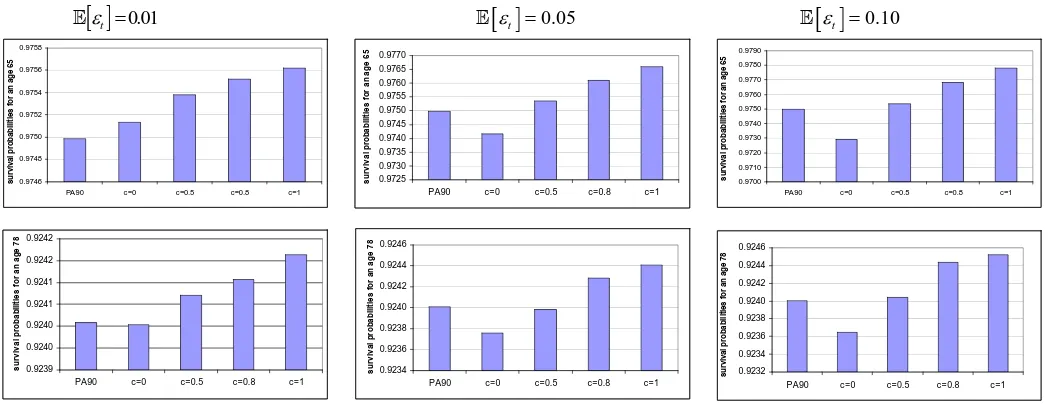
In Figure 2, we also provide the comparison between the CMI PA90 survival probability

values with the adjusted ones referring to ages 65 and 78 years, (similar results apply also for other

ages and for other tables; results are available from the authors).

The results shown in Figure 2 confirm those given in Figure 1: by increasing the parameter

c, the adjusted survival probabilities become higher than those from the CMI mortality table as the

probability that the sign of the mortality shock is negative decreases.

We also observe that, by assuming c = 0, the Continuous Mortality Investigation survival

probabilities can also be higher than the adjusted ones, especially by increasing the mean of the beta

distribution, since the effect of the mortality shock is stronger than that of the variable ν_t .

4.

Historical analysis

In this section in order to assess the goodness of the models set up in sections 2 and 3, we test the

full framework using historical values for mortality and interest rates, in a similar fashion to the

study performed by Ballotta and Haberman (2003) for guaranteed annuity options.

In our analysis we consider a hypothetical 25 year annuity contract issued in 1979 to a male

placeholder aged 65 years. In particular, we start by defining for the annuity contract under

examination the evolution over time until the present day of the historical market value. We then

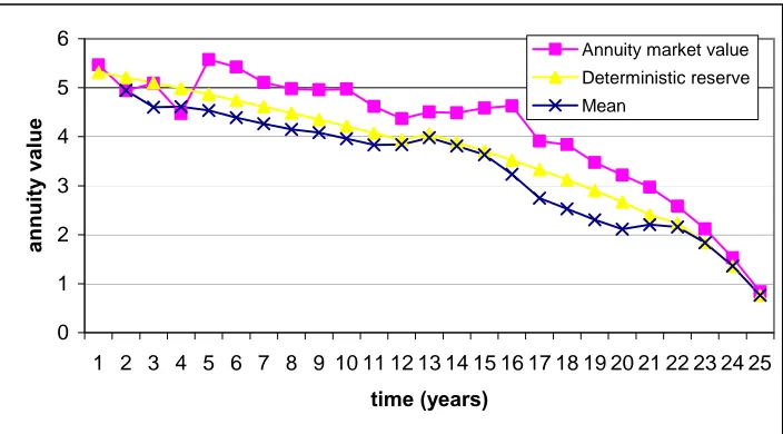
compare this to the deterministic reserve and the value obtained by using our framework.

The market value of the 25 year annuity contract is obtained by using the market value of

the zero coupon bonds with maturities corresponding to the annuity payment dates from 1979 to

2003, and the mortality tables in force over this period of time. Thus, the prices of the zero coupon

bonds in each year and for each maturity have been calculated using the prevailing market rates.

Further, the survival probabilities are calculated using the PA90 mortality table from 1979 to 1990,

the PMA80-C10 over the period 1991-1999, and the PMA92-C20 from year 2000. We also note

that, due to the construction of the contract and the type of analysis carried out, the unexpired term

of the annuity reduces from 25 year by year. The results presented in Figure 3 show how the market

[image:14.595.57.540.111.508.2]

Figure1: Comparison between PA90 table and adjusted tables obtained by varying the parameters of beta

distribution and the values of c.

1st _{case implies a beta distribution with mean equal to 0.01 and variance equal to 0.0081}

2nd _{case implies a beta distribution with mean equal to 0.05 and variance equal to 0.0407}

3rd _{case implies a beta distribution with mean equal to 0.10 and variance equal to 0.0814}

c = 0 c = 0.5

c = 0.8 c = 1

Figure 2: Comparison between CMI tables and adjusted tables by varying c and the parameters of beta

distribution

[ ]

ε_t =0.01

E E

[ ]

ε_t =0.05 E

[ ]

ε_t =0.10

-0.0005 0 0.0005 0.001 0.0015 0.002 0.0025

1 2 3 4 5 6 7 8 9 10111213141516171819202122232425 time (years) Ps90-Ps90new(1°case) Ps90-Ps90new(2°case) Ps90-Ps90new(3°case) -0.001 -0.0008 -0.0006 -0.0004 -0.0002 0 0.0002

1 2 3 4 5 6 7 8 9 10111213141516171819202122232425 time (years) Ps90-Ps90new(1°case) Ps90-Ps90new(2°case) Ps90-Ps90new(3°case) -0.002 -0.0018 -0.0016 -0.0014 -0.0012 -0.001 -0.0008 -0.0006 -0.0004 -0.0002 0

1 2 3 4 5 6 7 8 9 10111213141516171819202122232425 time (years) Ps90-Ps90new(1°case) Ps90-Ps90new(2°case) Ps90-Ps90new(3°case) -0.003 -0.0025 -0.002 -0.0015 -0.001 -0.0005 0

1 2 3 4 5 6 7 8 9 10111213141516171819202122232425 time (years) Ps90-Ps90new(1°case) Ps90-Ps90new(2°case) Ps90-Ps90new(3°case) 0.9746 0.9748 0.9750 0.9752 0.9754 0.9756 0.9758

PA90 c=0 c=0.5 c=0.8 c=1

su rv iv al p ro b ab ilit ie s f o r a n a g e 6 5 0.9240 0.9240 0.9241 0.9241 0.9242 0.9242 u rv iv a l pr oba bilit ie s f o r a n a g e 7 8 0.9725 0.9730 0.9735 0.9740 0.9745 0.9750 0.9755 0.9760 0.9765 0.9770

PA90 c=0 c=0.5 c=0.8 c=1

su rv ival p ro b a b ili ti es f o r an ag e 65 0.9236 0.9238 0.9240 0.9242 0.9244 0.9246 rv iv a l pr oba bilit ie s f o r a n a g e 7 8 0.9700 0.9710 0.9720 0.9730 0.9740 0.9750 0.9760 0.9770 0.9780 0.9790

PA90 c=0 c=0.5 c=0.8 c=1

[image:14.595.57.581.562.766.2]

The corresponding deterministic mathematical reserves are calculated using standard

techniques, i.e. by the expected present value of the future payments, where the discount rate is set

equal to the interest rate prevailing in the market at the inception of the contract, which in 1979 was

13% (source: Bank of England). The choice of this rate is justified by the fact that it can be

considered as the lower bound for any prudential discount rate. For the mortality rates, we adopt

the single-entry mortality tables that were being used in practice over this period of time, as noted

above: using the PA90 mortality table from 1979 to 1990, the PMA80-C10 over the period

1991-1999, and the PMA92-C20 from year 2000.

Finally, we compare the “historical annuity market values” with the central estimate of the

distribution of the annuity fair value, which is calculated using the financial approaches described in

section 2, whose parameters have been calibrated to the estimates of the UK yield curves provided

by the Bank of England (the full set of parameters is provided in the Appendix). Survival

probabilities are calculated using the corresponding mortality tables as described above.

Hence, Figures 4 and 5 show the comparison among the historical annuity market values,

the deterministic reserves and the central estimates of the fair value’s distribution calculated using

the CIR model and the HJM model. We note from the results that the annuity fair value calculated

on the basis of the CIR model provides the closest estimates to the “historical market value”;

however, we recognise that in general the estimated liabilities do not necessarily correspond to the

historical annuity prices.

In order to consider in the analysis the mortality risk as well, in Figures 6-9 we show the

comparison among the historical annuity market values, the deterministic reserves and the central

estimates of the fair value’s distribution calculated using, not only the CIR model and the HJM

model, but also the modified version of the stochastic mortality model developed by Lin and Cox

(2005) and described in section 3. In particular, we show only the results obtained by assuming c =

0 and c = 1 as similar conclusions can be obtained for the other assumptions as well (results are

available from the authors).

Similarly to the case of the results shown in Figures 4 and 5, we note that in general the

estimated liabilities do not reflect the market value. Hence, we conclude that an additional amount

should be added to the estimated mean value of the liabilities, in line with that suggested by the

IASB Insurance Project and the EU Solvency II Review, which define this amount as risk margin.

We observe that the appropriate approach for calculating the MVM is one of the key issues arising

from the IASB Insurance Project and the EU Solvency II Review, and is discussed in more detail in

[image:16.595.91.476.145.329.2]

Figure 3:Historical evolution of the market value of an annuity issued in 1979 to a male policyholder aged 65 years. The market consistent value is calculated in each year using the prices of the corresponding zero coupon bonds for each maturity corresponding to an annuity payment date. (Source for the market yield to maturity: bank of England website).

5.

The risk margin

The results of the previous section suggest how the measurement of insurance liabilities needs to

incorporate an additional amount arising from the uncertainty naturally associated with the

insurance business, and due to the necessary assumptions required in the fair valuation in the

absence of a deep liquid market.

As IASB suggests, the risk margin should reflect all of the risks associated with the liability.

The risk margin should be explicit in order to improve the quality of the estimate and the

transparency of the calculation method, and should consider the risks associated with both market

variables (such as interest rates which can be derived from market prices) and non market variables

(such as mortality). Therefore, the risk margin should be as consistent as possible with market

prices.

The IASB does not prescribe specific techniques in order to estimate the risk margin.

However, it is acknowledged, according to the Groupe Consultatif Actuariel Europeen (2006), that

the risk margin should be set as an addition to the best estimate, that it should capture uncertainty in

parameters, models and trends, that it should be harmonised across Europe and that it should

provide a sufficient level of policyholder protection together with capital requirements. 0

1 2 3 4 5 6

1 2 3 4 5 6 7 8 9 10 11 12 13 14 15 16 17 18 19 20 21 22 23 24 25

time (years)

H

ist

o

ri

c

al

a

n

n

u

it

y

m

a

rket

val

u

[image:17.595.118.478.143.339.2]

Figure 4: Comparison of the “historical annuity market values” with the mathematical reserves and the annuity fair values calculated using the CIR model.

0 1 2 3 4 5 6 7

1 2 3 4 5 6 7 8 9 10 11 12 13 14 15 16 17 18 19 20 21 22 23 24 25

time (years)

annuity value

Annuity market value Deterministic reserve Mean

Figure 5:Comparison of the “historical annuity market values” with the mathematical reserves and the annuity

fair values calculated using the HJM model.

0 1 2 3 4 5 6

1 2 3 4 5 6 7 8 9 10 11 12 13 14 15 16 17 18 19 20 21 22 23 24 25

time (years)

annuity value

[image:17.595.117.479.449.645.2]

Figure 6: Comparison of the “historical annuity market values” with the mathematical reserves and the annuity

fair values calculated using the CIR model and the stochastic mortality model with assumptions c = 0 and a

mean equal to 0.01 for the beta distribution of the mortality shock parameter.

0 1 2 3 4 5 6 7

1 2 3 4 5 6 7 8 9 10 11 12 13 14 15 16 17 18 19 20 21 22 23 24 25

time (years)

annuity value

[image:18.595.118.480.165.363.2]

Annuity market value Deterministic reserve Mean

Figure 7: Comparison of the “historical annuity market values” with the mathematical reserves and the annuity

fair values calculated using the HJM model and the stochastic mortality model with assumptions c = 0 and a

mean equal to 0.01 for the beta distribution of the mortality shock parameter.

0 1 2 3 4 5 6

1 2 3 4 5 6 7 8 9 10 11 12 13 14 15 16 17 18 19 20 21 22 23 24 25

time (years)

a

nnuity value

[image:19.595.119.478.203.400.2]

Figure 8: Comparison of the “historical annuity market values” with the mathematical reserves and the annuity

fair values calculated using the CIR model and the stochastic mortality model with assumptions c = 1 and a

mean equal to 0.01 for the beta distribution of the mortality shock parameter.

0 1 2 3 4 5 6 7

1 2 3 4 5 6 7 8 9 10 11 12 13 14 15 16 17 18 19 20 21 22 23 24 25

time (years)

annuity value

Annuity market value Deterministic reserve Mean

Figure 9: Comparison of the “historical annuity market values” with the mathematical reserves and the annuity

fair values calculated using the HJM model and the stochastic mortality model with assumptions c = 1 and a

mean equal to 0.01 for the beta distribution of the mortality shock parameter.

0 1 2 3 4 5 6

1 2 3 4 5 6 7 8 9 10 11 12 13 14 15 16 17 18 19 20 21 22 23 24 25

time (years)

annuity value

[image:19.595.121.473.510.705.2]

Different approaches are referred to or used by the insurance industry and some insurance

regulators. Examples are the cost of capital approach (see the Swiss Solvency Test (FOPI 2004))

which estimates the cost of holding the future required regulatory capital requirement, the percentile

approach which requires the fixing of an explicit confidence level, and a moments-based approach

which utilises multiples of one or more specific parameters (such as standard deviation, variance

and higher moments) of the estimated probability distribution.

In this section we analyse the percentile approach which was taken up by the EU

Commission and included in the Solvency 2 Roadmap and provided by CEIOPS as a working

hypothesis, and the standard deviation approach which is in line with the Australian Prudential

Regulation Authority (APRA).

In both cases, an insurer would need to simulate different scenarios or derive a formula

reflecting the probability distribution of cash flows.

5.1 The percentile approach

According to the percentile approach, the margin is calculated as the difference between the liability

amount at a prespecified confidence level, and the central estimate of fair value distribution. The

problem is to decide which particular percentile should be set as the standard.

The 75% confidence level is the level which is based on the precedent set in Australia. This

level has also been taken up by the EU Commission, and included in the Solvency 2 Roadmap, and

provided by CEIOPS as a working hypothesis. For completeness, in this study we also consider

other percentiles such as the 90th and 95th ones.

Our aim is to analyse the implication of each percentile in order to assess which confidence

level makes it possible to capture the historical market values.

In Figure 10, for ease of exposition, we only provide the comparison of the “historical

annuity market values” with the 75th, 90th, 95th percentile and the central estimate of the fair value

distribution obtained by using the CIR and HJM model and the adjusted survival probabilities.

Specifically, we consider the adjusted survival probabilities achieved by assuming c equal to 0 and

1 and a mean equal to 0.01 for the mortality shock (similar results are obtained by considering other

mortality assumptions).

From the plots of Figure 10, we note that the closest estimate to the historical market value

the 90th percentile in the case of the HJM model-based framework. By changing stochastic models

and the confidence level, the fair values change significantly.

The results show a strong dependency on the key assumptions for distributions, stochastic

models and input parameters. This is recognised by the industry as the main disadvantage of the

percentile approach and confirms how clear guidelines on the assumptions backing the fair

valuation are necessary in order to guarantee that the results of the percentile approach would be

comparable among insurance companies.

5.2 The standard deviation approach

According to the standard deviation approach, the risk margin is a percentage of the standard

deviation of the estimated reserve distribution. Thus, the overall estimate of the fair value could be

calculated as

σ µ+k

where µ is the liability’s best estimate (represented by the mean value); while k is a percentage of

the standard deviation, σ , of the best estimate’s distribution.

The problem which arises is the identification of what is the appropriate multiple of the

standard deviation capturing effectively the risk. In line with APRA’s approach we need to consider

at least 50% of the standard deviation, (Collings and White (2001)). For completeness, in this study

we also consider other percentages such as 100%, 150% and 200%.

In this section we want to analyse the effect of each percentage in order to assess which

multiple makes it possible to better capture the historical market values.

Hence, in Figure 11 we compare the “historical annuity market values” against the mean

added to different percentages of the standard deviation of the fair value distribution. In detail, we

consider the fair value distribution obtained by using the CIR and HJM model and the adjusted

survival probabilities achieved by assuming c equal to 0 and 1 and a mean equal to 0.01 for the

mortality shock (similar results are obtained by considering other mortality assumptions).

From the plots of Figure 11 we note that the closest estimate to the historical market value is

given by the multiple of standard deviation equal to 0.5 in the case of the valuation framework

based on the CIR model, and equal to 1.5 in the case of the HJM model-based framework. Hence,

with the standard deviation approach, as for the percentile approach shown in the previous section,

we observe that by varying stochastic models, the fair values and the relative risk margin change

[image:22.595.116.538.128.411.2]

Figure 10: Comparison of the “historical annuity market values” with the 75th_{, 90}th_{, 95}th _{percentile and the}

central estimate of the fair value distribution obtained by using the CIR and HJM model and the adjusted

survival probabilities (mean equal to 0.01 for the mortality shock and c = 0 and c = 1).

0 1 2 3 4 5 6 7 8 9 10111213141516171819202122232425 0 1 2 3 4 5 6 7 8 time (years)

CIR model; c = 0 Market value 75th percentile 90th percentile 95th percentile Central estimate

0 1 2 3 4 5 6 7 8 9 10111213141516171819202122232425 0 1 2 3 4 5 6 7 8 time (years)

CIR; c = 1 Market value

75th percentile 90th percentile 95th percentile Central estimate

0 1 2 3 4 5 6 7 8 9 10111213141516171819202122232425 0 1 2 3 4 5 6 7 8 time (years) HJM; c = 0

[image:22.595.118.534.471.753.2]

0 1 2 3 4 5 6 7 8 9 10111213141516171819202122232425 0 1 2 3 4 5 6 7 8 time (years) HJM; c = 1 Market value 75th percentile 90th percentile 95th percentile Central estimate Market value 75th percentile 90th percentile 95th percentile Central estimate

Figure 11: Comparison of the “historical annuity market values” with the mean added of different percentages of the standard deviation of the fair value distribution obtained by using the CIR and HJM model and the

adjusted survival probabilities (mean equal to 0.01 for the mortality shock and c = 0 and c = 1).

0 1 2 3 4 5 6 7 8 9 10111213141516171819202122232425 0 1 2 3 4 5 6 7 8 time (years) CIR; c = 0

0 1 2 3 4 5 6 7 8 9 10111213141516171819202122232425 0 1 2 3 4 5 6 7 8 time (years) CIR; c = 1

0 1 2 3 4 5 6 7 8 9 10111213141516171819202122232425 0 1 2 3 4 5 6 7 8 time (years) HJM; c = 0

0 1 2 3 4 5 6 7 8 9 10111213141516171819202122232425 0 1 2 3 4 5 6 7 8 time (years) CIR; c = 1 Market value

Mean + 0.5*st.d. Mean + st.d. Mean + 1.5* st.d. Mean + 2* st.d.

Market value Mean + 0.5* st.d. Mean + st.d. Mean + 1.5* st.d. Mean + 2* st.d.

Market value Mean + 0.5*st.d. Mean + st.d. Mean + 1.5* st.d. Mean + 2* st.d.

6. Concluding remarks

In this paper, we develop a market consistent valuation approach for the setting up of the reserve of

an annuity contract; the proposed approach incorporates the two main risks affecting the contract:

the interest rate risk and the mortality risk.

The behaviour of the annuity contract is analysed by considering two alternative frameworks for

interest rates based on the CIR model and the HJM model and a modified version of the stochastic

mortality model developed by Cox and Lin. We highlight the importance of the choice of the model

assumptions in the context of fair valuation, while not necessarily trying to identify the most correct

model for mortality and the financial market.

In the light of the analysis presented here, we identify areas where there is scope for further

work such as studying the effect of adopting alternative assumptions for the distributions used in the

mortality model.

Numerical results confirm the need, expressed by the IASB and the Solvency II project, for

a risk margin in the fair valuation in order to take into account the unavoidable uncertainty of the

insurance business and the presence of model risk and parameter risk.

Among the different approaches provided by practitioners, academics and regulators, for the

calculation of the risk margin for technical provisions, we consider both the percentile and the

standard deviation approach.

An important conclusion of the analysis is the sensitivity of the annuity fair values and the

risk margin to the underlying assumptions and choices made as part of calibration.

The results point to the need for clear guidelines and constraints in order to avoid areas of

subjectivity, such as models and calibration, which can lead to a wide variation of values from

company to company. Consequently, with the objective of guaranteeing more transparency,

consistency and comparability, we recognise that a common reference framework for the market

consistent valuation of the technical provisions and its components, such as the best estimate and

the risk margin, becomes a crucial requirement.

Acknowledgements

This project was supported by a research grant from the UK Actuarial Profession. Preliminary

results have been presented at the 10th International Congress in Insurance: Mathematics and

[image:24.595.108.490.155.528.2]

Appendix

Table 1: Parameter set for the interest rate models introduced in section 2.

CIR Model HJM Model

year θ κ ν r(0) σ b r(0)

1979 0.1202 0.10 0.0606 0.14 0.02925 0.10 0.14

1980 0.1226 0.10 0.0588 0.16 0.02925 0.10 0.16

1981 0.1206 0.10 0.0506 0.15 0.02466 0.10 0.15

1982 0.1300 0.10 0.0514 0.11 0.02327 0.10 0.11

1983 0.0768 0.10 0.0549 0.10 0.02424 0.10 0.10

1984 0.0968 0.10 0.0558 0.10 0.02464 0.10 0.10

1985 0.0737 0.10 0.0527 0.13 0.02464 0.10 0.13

1986 0.0977 0.10 0.0513 0.11 0.02320 0.10 0.11

1987 0.1081 0.10 0.0532 0.10 0.02320 0.10 0.10

1988 0.0946 0.10 0.0532 0.10 0.02320 0.10 0.10

1989 0.0414 0.12 0.0418 0.15 0.02118 0.12 0.15

1990 0.0519 0.12 0.0403 0.14 0.02020 0.12 0.14

1991 0.0805 0.12 0.0420 0.12 0.02028 0.12 0.12

1992 0.0877 0.12 0.0456 0.10 0.02085 0.12 0.10

1993 0.1273 0.10 0.0703 0.06 0.02787 0.10 0.06

1994 0.0862 0.08 0.0850 0.06 0.03158 0.08 0.06

1995 0.1370 0.08 0.0896 0.07 0.03386 0.08 0.07

1996 0.1249 0.08 0.0977 0.06 0.03627 0.08 0.06

1997 0.1192 0.08 0.0994 0.07 0.03756 0.08 0.07

1998 0.0579 0.10 0.0770 0.07 0.03143 0.10 0.07

1999 0.0334 0.10 0.0576 0.06 0.02246 0.10 0.06

2000 0.0413 0.12 0.0299 0.06 0.01256 0.12 0.06

2001 0.0409 0.15 0.0142 0.05 0.00628 0.15 0.05

References

1. Ballotta, L., Esposito, G., Haberman, S., (2006). The IASB Insurance Project for Life

Insurance Contracts; impact on reserving methods and solvency requirements. Insurance:

Mathematics and Economics,.39, 356-75.

2. Ballotta, L., Haberman, S., (2003). Valuation of guaranteed annuity conversion options.

Insurance: Mathematics and Economics, 33, 87-108.

3. Bank of England. Estimates of the UK Yield Curves,

http://213.225.136.206/statistics/yieldcurve/index.htm.

4. CEA, (2006). CEA Document of Cost of Capital, http://www.cea.assur.org.

5. Chiarella, C., Kwon O. K. (2001). Classes of interest rate models under the HJM

framework, Asia Pacific Financial Markets, 8, 1-22.

6. Collings, S.,White, G., (2001). APRA Risk Margin Analysis, Trowbridge Consulting.

Presented at the Institute of Actuaries of Australia XIIIth General Insurance Seminar,

November 2001.

7. Cox, J.C., Ingersoll, J.E, Ross, S.A., (1985). A theory of the term structure of interest rates.

Econometrica, 53, 385-407.

8. Cox, S.H., Lin, Y., (2005). Securitization of mortality risks in life annuities. The Journal of

Risk and Insurance,.72, 227-252.

9. FOPI, (2004). White Paper of the Swiss Solvency Test.

10.Group Consultatif Actuariel Europeen, (2006). Solvency II: Risk Margin Comparison.

11.Heath, D., Jarrow, R.A., Morton, A., (1992). Bond pricing and the term structure of interest

rates: a new methodology for contingent claims valuation. Econometrica, 60, 77–105.

12.Hull, J., White, A., (1990). Pricing Interest-Rate-Derivative Securities. The Review of

Financial Studies, 3, 573-592.

13.IAIS, (2006). Issues arising as a result of the IASB’s Insurance Contracts Project – Phase II

Second Set of IAIS Observations.

14.Jeffery, T., Olivier, P., (2004). Stochastic mortality: An Exploration. Presented to the

Society of Actuaries in Ireland.

15.Pollard, A.H. (1970). Random mortality fluctuations and the binomial hypothesis. Journal

of the Institute of Actuaries, 96, 251-264.

16.Vasicek, O., (1977). An equilibrium characterization of the term structure. Journal of

Actuarial Research Papers since 2001

Report Number

Date Publication Title Author

135. February 2001. On the Forecasting of Mortality Reduction Factors.

ISBN 1 901615 56 1

Steven Haberman Arthur E. Renshaw

136. February 2001. Multiple State Models, Simulation and Insurer Insolvency. ISBN 1 901615 57 X

Steve Haberman Zoltan Butt Ben Rickayzen

137. September 2001 A Cash-Flow Approach to Pension Funding. ISBN 1 901615 58 8

M. Zaki Khorasanee

138. November 2001 Addendum to “Analytic and Bootstrap Estimates of Prediction Errors in Claims Reserving”. ISBN 1 901615 59 6

Peter D. England

139. November 2001 A Bayesian Generalised Linear Model for the Bornhuetter-Ferguson Method of Claims Reserving. ISBN 1 901615 62 6

Richard J. Verrall

140. January 2002 Lee-Carter Mortality Forecasting, a Parallel GLM Approach, England and Wales Mortality Projections.

ISBN 1 901615 63 4

Arthur E.Renshaw Steven Haberman.

141. January 2002 Valuation of Guaranteed Annuity Conversion Options.

ISBN 1 901615 64 2

Laura Ballotta Steven Haberman

142. April 2002 Application of Frailty-Based Mortality Models to Insurance Data. ISBN 1 901615 65 0

Zoltan Butt Steven Haberman

143. Available 2003 Optimal Premium Pricing in Motor Insurance: A Discrete Approximation.

Russell J. Gerrard Celia Glass

144. December 2002 The Neighbourhood Health Economy. A Systematic Approach to the Examination of Health and Social Risks at Neighbourhood Level. ISBN 1 901615 66 9

Les Mayhew

145. January 2003 The Fair Valuation Problem of Guaranteed Annuity Options : The Stochastic Mortality Environment Case.

ISBN 1 901615 67 7

Laura Ballotta Steven Haberman

146. February 2003 Modelling and Valuation of Guarantees in With-Profit and Unitised With-Profit Life Insurance Contracts.

ISBN 1 901615 68 5

Steven Haberman Laura Ballotta Nan Want

147. March 2003. Optimal Retention Levels, Given the Joint Survival of Cedent and Reinsurer. ISBN 1 901615 69 3

Z. G. Ignatov Z.G., V.Kaishev

R.S. Krachunov

148. March 2003. Efficient Asset Valuation Methods for Pension Plans.

ISBN1 901615707 M. Iqbal Owadally

V. Kaishev

151. August 2004 Application of Stochastic Methods in the Valuation of Social Security Pension Schemes. ISBN 1 901615 72 3

Subramaniam Iyer

152. October 2003. Guarantees in with-profit and Unitized with profit Life Insurance Contracts; Fair Valuation Problem in Presence of the Default Option1. ISBN 1-901615-73-1

Laura Ballotta Steven Haberman Nan Wang

153. December 2003 Lee-Carter Mortality Forecasting Incorporating Bivariate Time Series. ISBN 1-901615-75-8

Arthur E. Renshaw Steven Haberman

154. March 2004. Operational Risk with Bayesian Networks Modelling.

ISBN 1-901615-76-6

Robert G. Cowell Yuen Y, Khuen Richard J. Verrall

155. March 2004. The Income Drawdown Option: Quadratic Loss.

ISBN 1 901615 7 4

Russell Gerrard Steven Haberman Bjorn Hojgarrd Elena Vigna

156. April 2004 An International Comparison of Long-Term Care

Arrangements. An Investigation into the Equity, Efficiency and sustainability of the Long-Term Care Systems in Germany, Japan, Sweden, the United Kingdom and the United States. ISBN 1 901615 78 2

Martin Karlsson Les Mayhew Robert Plumb Ben D. Rickayzen

157. June 2004 Alternative Framework for the Fair Valuation of

Participating Life Insurance Contracts. ISBN 1901615-79-0

Laura Ballotta

158. July 2004. An Asset Allocation Strategy for a Risk Reserve considering both Risk and Profit. ISBN 1 901615-80-4

Nan Wang

159. December 2004 Upper and Lower Bounds of Present Value Distributions of Life Insurance Contracts with Disability Related Benefits. ISBN 1 901615-83-9

Jaap Spreeuw

160. January 2005 Mortality Reduction Factors Incorporating Cohort Effects.

ISBN 1 90161584 7

Arthur E. Renshaw Steven Haberman

161. February 2005 The Management of De-Cumulation Risks in a Defined Contribution Environment. ISBN 1 901615 85 5.

Russell J. Gerrard Steven Haberman Elena Vigna

162. May 2005 The IASB Insurance Project for Life Insurance Contracts: Impart on Reserving Methods and Solvency

Requirements. ISBN 1-901615 86 3.

Laura Ballotta Giorgia Esposito Steven Haberman

163. September 2005 Asymptotic and Numerical Analysis of the Optimal Investment Strategy for an Insurer. ISBN 1-901615-88-X

Paul Emms Steven Haberman

164. October 2005. Modelling the Joint Distribution of Competing Risks Survival Times using Copula Functions. I SBN 1-901615-89-8

Vladimir Kaishev Dimitrina S, Dimitrova Steven Haberman

165. November 2005.

Excess of Loss Reinsurance Under Joint Survival Optimality. ISBN1-901615-90-1

Vladimir K. Kaishev Dimitrina S. Dimitrova

166. November 2005.

Lee-Carter Goes Risk-Neutral. An Application to the Italian Annuity Market.

Population. ISBN 1-901615-93-6 Maria Russolillo

168. February 2006 The Probationary Period as a Screening Device: Competitive Markets. ISBN 1-901615-95-2

Jaap Spreeuw Martin Karlsson

169. February 2006 Types of Dependence and Time-dependent Association between Two Lifetimes in Single Parameter Copula Models. ISBN 1-901615-96-0

Jaap Spreeuw

170. April 2006 Modelling Stochastic Bivariate Mortality

ISBN 1-901615-97-9

Elisa Luciano Jaap Spreeuw Elena Vigna.

171. February 2006 Optimal Strategies for Pricing General Insurance.

ISBN 1901615-98-7

Paul Emms Steve Haberman Irene Savoulli

172. February 2006 Dynamic Pricing of General Insurance in a Competitive Market. ISBN1-901615-99-5

Paul Emms

173. February 2006 Pricing General Insurance with Constraints.

ISBN 1-905752-00-8

Paul Emms

174. May 2006 Investigating the Market Potential for Customised Long Term Care Insurance Products. ISBN 1-905752-01-6

Martin Karlsson Les Mayhew Ben Rickayzen

175. December 2006 Pricing and Capital Requirements for With Profit Contracts: Modelling Considerations. ISBN 1-905752-04-0

Laura Ballotta

176. December 2006 Modelling the Fair Value of Annuities Contracts: The Impact of Interest Rate Risk and Mortality Risk. ISBN 1-905752-05-9

Laura Ballotta Giorgia Esposito Steven Haberman

Statistical Research Papers

Report Number

Date Publication Title Author

1. December 1995. Some Results on the Derivatives of Matrix Functions. ISBN

1 874 770 83 2

P. Sebastiani

2. March 1996 Coherent Criteria for Optimal Experimental Design.

ISBN 1 874 770 86 7

A.P. Dawid P. Sebastiani

3. March 1996 Maximum Entropy Sampling and Optimal Bayesian

Experimental Design. ISBN 1 874 770 87 5

P. Sebastiani H.P. Wynn

4. May 1996 A Note on D-optimal Designs for a Logistic Regression

Model. ISBN 1 874 770 92 1

P. Sebastiani R. Settimi

5. August 1996 First-order Optimal Designs for Non Linear Models.

ISBN 1 874 770 95 6

P. Sebastiani R. Settimi

6. September 1996 A Business Process Approach to Maintenance:

Measurement, Decision and Control. ISBN 1 874 770 96 4

10. March 1997. Guidelines for Corrective Replacement Based on Low Stochastic Structure Assumptions. ISBN 1 901615 01 4.

M.J. Newby F.P.A. Coolen

11. March 1997 Approximations for the Absorption Distribution and its

Negative Binomial Analogue. ISBN 1 901615 02 2

Martin J. Newby

12. June 1997 The Use of Exogenous Knowledge to Learn Bayesian

Networks from Incomplete Databases. ISBN 1 901615 10 3

M. Ramoni P. Sebastiani

13. June 1997 Learning Bayesian Networks from Incomplete Databases.

ISBN 1 901615 11 1

M. Ramoni P.Sebastiani

14. June 1997 Risk Based Optimal Designs. ISBN 1 901615 13 8 P.Sebastiani

H.P. Wynn

15. June 1997. Sampling without Replacement in Junction Trees.

ISBN 1 901615 14 6

Robert G. Cowell

16. July 1997 Optimal Overhaul Intervals with Imperfect Inspection and

Repair. ISBN 1 901615 15 4

Richard A. Dagg Martin J. Newby

17. October 1997 Bayesian Experimental Design and Shannon Information.

ISBN 1 901615 17 0

P. Sebastiani. H.P. Wynn

18. November 1997. A Characterisation of Phase Type Distributions.

ISBN 1 901615 18 9

Linda C. Wolstenholme

19. December 1997 A Comparison of Models for Probability of Detection (POD)

Curves. ISBN 1 901615 21 9

Wolstenholme L.C

20. February 1999. Parameter Learning from Incomplete Data Using Maximum

Entropy I: Principles. ISBN 1 901615 37 5

Robert G. Cowell

21. November 1999 Parameter Learning from Incomplete Data Using Maximum

Entropy II: Application to Bayesian Networks. ISBN 1 901615 40 5

Robert G. Cowell

22. March 2001 FINEX : Forensic Identification by Network Expert

Systems. ISBN 1 901615 60X

Robert G.Cowell

23. March 2001. Wren Learning Bayesian Networks from Data, using

Conditional Independence Tests is Equivalant to a Scoring Metric ISBN 1 901615 61 8

Robert G Cowell

24. August 2004 Automatic, Computer Aided Geometric Design of

Free-Knot, Regression Splines. ISBN 1-901615-81-2

Vladimir K Kaishev, Dimitrina S.Dimitrova, Steven Haberman Richard J. Verrall

25. December 2004 Identification and Separation of DNA Mixtures Using Peak

Area Information. ISBN 1-901615-82-0

R.G.Cowell S.L.Lauritzen J Mortera,

26. November 2005. The Quest for a Donor : Probability Based Methods Offer

Help. ISBN 1-90161592-8

P.F.Mostad T. Egeland., R.G. Cowell V. Bosnes Ø. Braaten

27. February 2006 Identification and Separation of DNA Mixtures Using Peak

Area Information. (Updated Version of Research Report

28. October 2006 Geometrically Designed, Variable Knot Regression Splines : Asymptotics and Inference. ISBN 1-905752-02-4

Vladimir K Kaishev, Dimitrina S.Dimitrova, Steven Haberman Richard J. Verrall

29. October 2006 Geometrically Designed, Variable Knot Regression

Splines : Variation Diminishing Optimality of Knots.

ISBN 1-905752-03-2

Vladimir K Kaishev, Dimitrina S.Dimitrova, Steven Haberman Richard J. Verrall

Faculty of Actuarial Science and Insurance

Actuarial Research Club

The support of the corporate members

•

CGNU Assurance

•

English Matthews Brockman

•

Government Actuary’s Department

is gratefully acknowledged.

Copyright 2006 © Faculty of Actuarial Science and Insurance, Cass Business School

106 Bunhill Row, London EC1Y 8TZ.