Transporting functions across ornaments

Transporting Functions across Ornaments

Pierre-Evariste Dagand Inria

Conor McBride University of Strathclyde

(e-mail:[email protected],[email protected])

Abstract

Programming with dependent types is a blessing and a curse. It is a blessing to be able to bake invariants into the definition of datatypes: we can finally write correct-by-construction software. However, this extreme accuracy is also a curse: a datatype is the combination of a structuring medium together with a special purpose logic. These domain-specific logics hamper any attempt to reuse code across similarly structured data.

In this article, we capitalise on the structural invariants of datatypes. To do so, we first adapt the notion of ornament to our universe of inductive families. We then show how code reuse can be achieved by ornamenting functions. Using these functional ornaments, we capture the relationship between functions such as the addition of natural numbers and the concatenation of lists. With this knowledge, we demonstrate how the implementation of the former informs the implementation of the latter: the user can ask the definition of addition to be lifted to lists and she will only be asked the details necessary to carry on adding lists rather than numbers.

Our presentation is formalised in a type theory with a universe of datatypes and all our constructions have been implemented as generic programs, requiring no extension to the type theory.

1 Introduction

Imagine designing a library for an ML-like language. For instance, we start with natural numbers and their operations, then we move to binary trees, then rose trees,etc.It is the garden of Eden: datatypes are data-structures, each coming with its unique and optimised set of operations. If we move to a language with richer datatypes, such as a dependently-typed language, we enter the Augean stables. Where we used to have binary trees, now we have complete binary trees, red-black trees, AVL trees, and countless other variants. Worse, we have to duplicate code across these tree-like datatypes: because they are defined upon this common binarily branching structure, a lot of computationally identical operations will have to be duplicated for the type checker to be satisfied.

Since their first introduction in ML, datatypes have evolved: besides providing an organisingstructure for computation, they are now offering morecontrolover what is a valid result. With richer datatypes, we can enforce invariants on top of the data-structures. In such a system, programmers strive to express the correctness of their programs in the types: a well-typed program is correctby construction.

Refinement types (Freeman & Pfenning, 1991; Swamyet al., 2011) are another technique to equip data-structures with rich invariants. In a dependently-typed setting, refinement types are expressible in terms of Σ-types. As such, they offer a clear-cut separation between the data (what is predicated upon, i.e. the first projection of theΣ-type) and the logic (the predicate,i.e.the second projection of theΣ-type). This approach benefits from a straightforward compilation strategy, which simply erases the refining predicates. Atkeyet al.(2012) have shown how refinement types relate to inductive families.

1.1 Ornaments?

However, these carefully crafted datatypes are a threat to any library design: the same data-structureis used for logically incompatible purposes. This explosion of specialised datatypes is overwhelming: these objects are too specialised to fit in a global library. Yet, because they share this common structure, many operations on them are extremely similar, if not exactly the same. To address this issue, McBride (2013) developedornaments, describing how one datatype can be enriched into anotherwith the same structure. Such structure-preserving transformations take two forms. First, we canextendthe initial type with more information.

1.1 Example(Ornament: Extending the Booleans to the option type). We can extend the Booleans to the option type by attaching ana:Ato the constructortrue:

dataBool:SETwhere

Bool 3true

| false

Maybe-OrnA

⇒

dataMaybe[A:SET]:SETwhere

MaybeA 3just(a:A) | nothing

4

1.2 Example(Ornament: Extending numbers to lists). Or we can extend natural numbers to lists by inserting ana:Aat each successor node:

dataNat:SETwhere

Nat 30

| suc(n:Nat)

List-OrnA

⇒

dataList[A:SET]:SETwhere

ListA 3nil

| cons(a:A)(as:ListA)

4

Second, we canrefine the indexing of the initial type, following a finer discipline. By refining the indices of a datatype, we make it logically more discriminating.

1.3 Example(Ornament: Refining numbers to finite sets). We refine natural numbers to finite sets by indexing the number with an upper-bound:

dataNat:SETwhere

Nat 30

| suc(n:Nat)

Fin-Orn ⇒

dataFin(n:Nat):SETwhere

Fin(n=sucn0)3f0(n0:Nat)

| fsuc(n0:Nat)(k:Finn0)

Put otherwise, the datatypeFinnis a type of cardinalityn.

4

1.4 Example(Ornament: Extending and refining numbers to vectors). We extend natural numbers to lists while refining the index to represent the length of the list thus constructed:

dataNat:SETwhere

Nat 30

| suc(n:Nat)

VecOA =⇒

dataVec[A:SET](n:Nat):SETwhere

VecA (n=0) 3nil

VecA(n=sucn0)3cons(n0:Nat)(a:A)(vs:VecA n0)

Note that we declare datatype parameters in brackets –e.g.,[A:SET]– and datatype indices in paren-theses –e.g.,(n:Nat). We make equational constraints on the latter only when needed, and explicitly – e.g.,(n=sucn0). We come back to the notation for inductive definitions in Section 3.3.

4

Because of their constructive nature, ornaments are not merely identifying similar structures: they give an effective recipe to build new datatypes from old, guaranteeing by construction that the structure is preserved. Hence, we can obtain a plethora of new datatypes with minimal effort.

1.2 Functional ornaments!

Whilst we have a good handle on the transformation of individual datatypes, we are still facing a major reusability issue: a datatype often comes equipped with a set of operations. Ornamenting this datatype, we have to entirely re-implement many similar operations. For example, the datatypeNatcomes with operations such as addition and subtraction. When defining lists as an ornament of natural numbers, it seems natural to transport the structure-preserving functions of NattoListA, such as moving from addition of natural numbers to concatenation of lists:

(m:Nat)+(n:Nat) : Nat

0 + n 7→n

(sucm) + n 7→suc(m+n)

⇒

(xs:ListA)++(ys:ListA) : ListA

nil ++ ys 7→ys

(consa xs)++ ys 7→consa(xs++ys)

or, from subtraction of natural numbers to dropping a prefix:

(m:Nat)−(n:Nat) : Nat

0 − n 7→0

m − 0 7→m

(sucm) − (sucn) 7→m−n

⇒

drop(xs:ListA) (n:Nat) : ListA

drop nil n 7→nil

drop xs 0 7→xs

drop(consa xs) (sucn) 7→dropxs n

More interestingly, the function we start with may involve several datatypes, each of which may be ornamented differently. In this paper, we develop the notion offunctional ornamentas a generalisation of ornaments to functions:

• We manually transport the comparison of numbers to the list lookup function in Section 2. This example provides the impetus for the rest of this article: we aim at explaining the structure behind it, generalise, and automate it;

• For this article to be self-contained, we recall the type theoretic foundations (Chapmanet al., 2010) upon which this article builds in Section 3. We strive to provide an intuition for our universe-based presentation of datatypes, and describe a convenient notation for inductive definitions;

• We describe how functions can be transported through functional ornaments. We formalise the concept of functional ornament by a universe construction in Section 5. Based on this universe, we establish the connection between a base function (such as addition and subtraction) and its ornamented version (such as, respectively,−++−anddrop). Within this framework, we redevelop the example of Section 2 with all the automation offered by our framework;

• In Section 6, we provide further support to drive the computer into lifting functions. As we can see from our examples above, the lifted functions often follow the same recursion pattern and return similar constructors: with a few smart constructors, we shall remove further clutter from our libraries.

This article is an exercise in constructive mathematics: upon identifying an isomorphism, we shall look at it with our constructive glasses and obtain an effective procedure to cross it. It is crucial to note that this article is built entirelywithintype theory. No change or adaptation to the meta-theory is required. In particular, the validity of our constructions is justified by mere type checking.

1.5 Remark (Notations). We shall write our code in a syntax inspired by the Epigram programming language (McBride & McKinna, 2004). For an optimal experience, we recommend reading the colour version of this article, available on Dagand’s webpage. Colours are used to classify the terms of the type theory. We also make use of theby(⇐) andreturn(7→) programming gadgets, further extending them to account for the automatic lifting of functions. For brevity, we write pattern-matching definitions when the recursion pattern is evident and unremarkable.

As in ML, unbound variables in type signatures are universally quantified, further abating syntactic noise. For higher-order functions, we indicate the implicit arguments with the quantifier∀x.(. . .)– or its annotated variant∀x:T.(. . .)– as follows:

example(op:∀n.VecA n→1) (xs:VecA k) (ys:VecA l):op xs=op ys

· · ·

Because we implicitly quantify over unbound type variables, these variables are not explicitly bound in the definition. We rely on the convention that these implicit arguments are automatically in scope of the definition, using the same variable name. For example, in the following definition,nis universally quantified in the type declaration and is in scope in the definition oflengthVec:

lengthVec(vs:VecA n) : Nat lengthVec vs 7→n

The syntax of datatype definitions draws upon the ML tradition as well: its novelty will be presented by way of examples in Section 3. Following mathematical usage, we shall extensively use mixfix operators, i.e.operators in prefix, infix, postfix, or closed form.

All the constructions presented in this article have been modelled in Agda, using only standard induc-tive definitions and two levels of universes. Rather than presenting the machine-checked code, we have chosen to use an high-level notation. This notation relies on the reader’s ability to cope with ambiguity. We shall therefore indulge in many abuse of language, as is common in mathematics. This allows us to focus on conveying ideas to the reader, rather than on satisfying a type checker. Throughout this article, we relate the high-level definitions to their Agda counterparts using a MODELfootnote indicating their location. For an absolutely formal treatment, we therefore refer the reader to the companion formalisation. The formalisation is available on Dagand’s website.

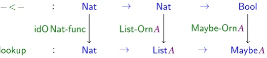
(m:Nat)<(n:Nat) : Bool m < 0 7→false 0 < (sucn) 7→true

(sucm) < (sucn) 7→m<n

?

=⇒

lookup(m:Nat) (xs:ListA) : MaybeA lookup m nil 7→nothing lookup 0 (consa xs)7→justa lookup (sucn) (consa xs)7→lookupn xs

Fig. 1: Implementation of−<−andlookup

A shorter version of this article has appeared in the proceedings of ICFP 2012 (Dagand & McBride, 2012). This version benefits from several presentational modifications to include significantly more ex-amples (in particular, in Section 3 and Section 4). The running example – lifting the comparison function of natural numbers – is also complemented by another example, lifting the addition of natural numbers. Worked out examples, throughout the paper, shall help the reader build a strong intuition of the generic constructions at play. We have also extended the original paper with new material. In Section 4.2, we cast the forcing and detagging transformations of Brady et al. (Bradyet al., 2003) in our universe of datatypes. Using these intuitions, we have streamlined the definition of reornaments and discuss the limits of iterating reornaments (Section 4.5). We have extended the lifting of recursion patterns to handle induction and case analysis (Section 6). Our treatment of the lifting of constructors (Section 6) has also treated in more details and its underlying mechanisms has been thoroughly illustrated.

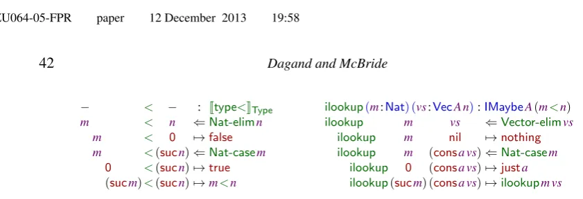
2 From Comparison to Lookup, Manually

There is an astonishing resemblance between the comparison function−<−on numbers and the list

lookupfunction (Fig. 1). Interestingly, the similarity is not merely at the level of types. It is also in their implementation: their definition follows the same pattern of recursion (first, case analysis on the second argument; then induction on the first argument) and they both return a failure value (respectively,false andnothing) in the first case analysis and a success value (respectively,trueandjust) in the base case of the induction.

This raises the question: whatexactlyis the relation between−<−andlookup? Also, could we use the implementation of−<−to guide the construction oflookup? First, let us work out the relation at the type level. To this end, we use ornaments to explain how each individual datatype has been promoted when going from−<−tolookup:

−<− Nat Nat Bool

lookup Nat ListA MaybeA

idO Nat-func List-OrnA Maybe-OrnA

: → →

: → →

Note that the first argument is ornamented to itself, or put differently, it has been ornamented by the identity ornamentidO(Definition 4.9, p.20).

Each of these ornaments come with a forgetful map:

length(as:ListA) : Nat length nil 7→0

length(consa as)7→suc(lengthas)

isJust(m:MaybeA) : Bool isJust nothing 7→false

As we shall see in Section 4.3, the forgetful maps can be automatically derived from the ornament definition.

Using these forgetful maps we deduce a relation, at the operational level, between−<−andlookup. This relation is uniquely determined by the ornamentation of the individual datatypes. Thiscoherence propertyis expressed as follows

(n:Nat)(xs:ListA)→isJust(lookupn xs)=n<lengthxs

or, equivalently, using a commuting diagram:

Nat×ListA MaybeA

Nat×Nat Bool

−<− lookup

id×length isJust

2.1 Remark(Vocabulary). We call the function we start with thebase function(here,−<−), its type be-ing thebase type(here,Nat→Nat→Bool). The richer function type built by ornamenting the individual pieces is called thefunctional ornament1of the base type (here,Nat→ListA→MaybeA). A function inhabiting this type is called alifting(here, lookup). A lifting is said to becoherent if it satisfies the coherence property.

♦ 2.2 Remark(Coherence and functional ornament). It is crucial to understand that the coherence of a lifting is relative to a given functional ornament: the same base function ornamented differently would give rise to a different coherence property.

For example, the base typeNat→Nat→Natcan be functionally ornamented to

Nat→ListA→ListA

for whichdropis a coherent solution with respect to−−−. However, it can also be functionally orna-mented to

ListA→ListA→ListA

for which −++− is a coherent solution with respect to −+−. Nonetheless, the two solutions are exclusive:dropis not coherent with respect to−+−, nor is−++−coherent with respect to−−−.

♦ We now have a better grasp of the relation between the base function and its lifting. However,lookup

remains to be implemented while making sure that it satisfies the coherence property. Traditionally, one would stop here: we would implementlookupand prove the coherence as a theorem. This works rather well in a system like Coq since it offers a powerful theorem proving environment. It does not work so well in a system like Agda that does not offer tactics to its users, forcing them to write explicit proof terms. It would not work at all in an ML language with GADTs, which has no notion of proof.

Historically, Coq has been engineered to specify (simply-typed) programs using (dependently-typed) propositions (Paulin-Mohring, 1989). This paradigm started shifting with languages such as Epigram,

Cayenne, or Agda: these systems offer an environment for dependently-typed programming. In this setting, the approach that consists in writing a simply-typed programming to prove it correct after the factfeels utterly laborious. If we have dependent types, why should we use them only forproofs, as an afterthought? A dependently-typed programming environment lets us write a lookup functioncorrect by construction: by implementing a more finely indexed version oflookup, the user drives the type checker into verifying the necessary invariants. This article is an exploration of this paradigm, in which we develop techniques to relieve the dependently-typed programmer from the burden of proofs.

To get the computer to work for us, we would rather implement the functionilookup

ilookup(m:Nat) (vs:VecA n) : IMaybeA(m<n)

ilookup m nil 7→nothing

ilookup 0 (consa vs) 7→justa

ilookup (sucm) (consa vs) 7→ilookupm vs

whereIMaybeAis the option type indexed by the truth value computed byisJust. It is defined as follows

dataIMaybe[A:SET](b:Bool):SETwhere

IMaybeA(b=true)3just(a:A) IMaybeA(b=false)3nothing

and it comes with a forgetful map:

forgetIMaybe(ima:IMaybeA b) : (ma:MaybeA)×isJustma=b

forgetIMaybe (justa) 7→(justa,refl)

forgetIMaybe nothing 7→(nothing,refl)

2.3 Remark. We overload the constructors ofMaybeandIMaybe: for a bi-directional type checker, there is no ambiguity as constructors are checked against their type.

♦ The rationale behindilookupis toindexthe types oflookupby their unornamented version. In effect, we index the types of its arguments by the (respective) argumentsm:Natandn:Natof−<−and we index the type of its result bym<n. By doing so, we can make sure that the result computed byilookup

respects the output of−<−on the unornamented indices: the result is necessarily correct,by indexing! The type ofilookupis naturally derived from the ornamentation of−<−intolookupand is uniquely determined by the functional ornament we start with. We shall automate its construction in Section 5.3 with the notion ofpatch(Definition 5.15).

2.4 Remark (Vocabulary). Expanding further our vocabulary, such a finely indexed function that is coherent by construction is called acoherent liftings.

We had separately introduced the notion ofliftingandcoherencein Remark 2.1, with the idea that a lifting is not necessarily coherent. Here, we are defining thecoherent liftingas those liftings that are coherent by construction. In fact, we shall establish in Theorem 5.19 that a lifting satisfying the coherence condition is isomorphic to a coherent lifting. There is therefore no ambiguity in identifying both notions of a “coherent lifting” and of a “lifting satisfying the coherence condition”.

♦ Ko and Gibbons (2011) use ornaments to specify the coherence requirements for functional liftings, but we work the other way around. Fromilookup, we extract thelookupfunction

lookup(m:Nat) (xs:ListA) : MaybeA

and its proof of correctness

cohLookup(n:Nat) (xs:ListA) : isJust(lookupn xs)=n<lengthxs

cohLookup m xs 7→π1(forgetIMaybe(ilookupm(makeVecxs)))

wheremakeVec:(xs:ListA)→VecA(lengthxs)turns a list into a vector of the corresponding length. Operationally, it is an identity. In Section 4.4, we show that it can be automatically derived from the ornament of lists.

The construction oflookupandcohLookupfeels automatic: we shall see in Section 5.4 howlookup

can automatically be obtained bypatching(Definition 5.22), whilecohLookupis merely an instance of a genericcoherenceresult (Definition 5.23).

2.5 Remark(ilookupvs. vlookup). The functionilookup is very similar to the more familiarvlookup

function:

vlookup(m:Finn) (vs:VecA n) : A

vlookup f0 (consa xs) 7→a

vlookup (fsucn) (consa xs) 7→vlookupn xs

These two definitions are actually equivalent, thanks to the isomorphism

(m:Nat)→IMaybeA(m<n) ∼= Finn→A

where we silently lift the boolean predicatem<n at the type-level, as is common practice in SSRE-FLECT (Gonthieret al., 2008) for instance.

Intuitively, we can move the constraint “m<n” from the result – where we return an object of type

IMaybeA(m<n)– to the premise – where we expect an object of typeFinn. Indeed, we can think of the typeFinnas the combination of a numberm:Nattogether with a proof thatm<n.

♦ With this example, we have manually unfolded the key steps of the construction of a lifting of−<−. Let us recapitulate each steps:

• Start with abase function, here−<−:Nat→Nat→Bool;

• Ornament its inductive components as desired, hereNattoListAandBooltoMaybeAin order to describe the lifting of interest, herelookup:Nat→ListA→MaybeAsatisfying

(n:Nat)(xs:ListA)→isJust(lookupn xs)=n<lengthxs

• Implement a carefully indexed version of the lifting, here

ilookup:(m:Nat)(vs:VecA n)→IMaybeA(m<n)

• Derive the lifting, herelookup, and its coherence proof, withoutwritinga proof!

Besides,ilookupis a useful addition to our library: it corresponds to the familiar vector lookup function, a function that one would have implemented anyway. Thus,ilookupis not just some scaffolding necessary to definelookup, it is a purposeful operation on its own.

This manual unfolding of the lifting is instructive: it involves many constructions on datatypes (here, the datatypesListAandMaybeA) as well as on functions (here, the type ofilookup, the definition of

3 A Universe of Datatypes

In dependently-typed systems such as Coq or Agda, datatypes are an external entity: each datatype definition extends the type theory with new introduction and elimination forms. The validity of a datatype definition is guaranteed by a positivity-checker that is part of the meta-theory of the proof system. A consequence is that, from within the type theory, it is not possible to create or manipulate inductive definitions, since they belong to the meta-theory.

In previous work (Chapmanet al., 2010), we have shown how to internalise inductive families into type theory. The practical outcome of this approach is that we can manipulate datatype declarations as first-class objects. We can program over the grammar of datatypes and, in particular, we can compute new datatypes from old. This is particularly useful to formalise the notion of ornament entirely within type theory. This also has a theoretical outcome: we do not need to prove meta-theoretical properties of our constructions, we can work in our type theory and use its logic as a formal system.

3.1 Remark(Theoryvs.meta-theory). The constructions described in this article arealsoapplicable in a setting where datatype definitions arenot internalised: all our constructions could be justified at the meta-level and then be syntactically presented in a language, such as, say, Agda, Coq, or an ML with GADTs. Working with an internalised presentation, we can simply avoid these two levels of logic and work in the logic provided by type theory.

Our requirements on the ambient type theory are boxed in a TYPE THEORY frame (e.g., Fig. 2, p.10), whilst constructions within that type theory are boxed in a DEFINITIONframe (e.g., Fig. 3, p.17). Because our work is grounded in an intensional reading of extensional isomorphisms, we box the original, extensional results in META-THEOREMframes (e.g., Equation 4.20, p.24). The proof of these results are absent from our (intensional) Agda model. Examples illustrating the various concepts are left unboxed.

♦

3.1 The type theory

Following our previous work, our requirements on the type theory are minimal: we will needΣ-types, Π-types, the unit set1, and at least two universes,SETandSET1.Σ-types are denoted(a:A)×B, introduced by pairs(x,y)and eliminated by first and second projections, respectivelyπ0andπ1.Π-types are denoted

(a:A)→B, introduced byλx.band eliminated by function application. The unit set is (uniquely) inhabited by∗. For convenience, we require theη-laws for the unit set,Σ-types (i.e.surjective pairing), andΠ-types to hold definitionally. Whenxis not free inB, we use the following abbreviations:

(x:A)→B_,A→B

(x:A)×B_,A×B

Hence obtaining the (non dependent) implication and conjunction from the dependent quantifiers. For convenience, we ask for our type theory to supportenumerationsof tags. We shall not dwell on their type theoretic definition, which can be found elsewhere (Dagand, 2013). We declare a (finite) enumeration of tags ’a,’b, and ’c by writing {’a’b’c}. Similarly, we define functions from such a collection by exhaustively enumerating the returned values, using the notation

{’a 7→ea,’b7→eb,’c7→ec}

When the cases are vertically aligned, we shall skip the separating commas.

dataIDesc[I:SET]:SET1where IDescI3var(i:I)

| 1

| Π(S:SET) (T:S→IDescI)

| Σ(S:SET) (T:S→IDescI)

J(D:IDescI)K(X:I→SET):SET JvariK X7→X i

J1K X7→1

JΠS TKX7→(s:S)→JT sKX JΣS TKX7→(s:S)×JT sKX TYPE THEORY

Fig. 2: Universe of inductive families

indexed datatypes, we also require our equality to satisfy the K rule (McBride, 1999),i.e.reflis the unique inhabitants of a propositional equality.

3.2 Universe of descriptions

We internalise inductive families by a universe construction. The role of this universe is todescribe signature functors overSETindexed byI,i.e.functors fromSETItoSETI. However, up to some currying-uncurrying, this type is subject to the isomorphism

SETI→SETI,(I→SET)→(I→SET)

∼

=I→(I→SET)→SET

that lets us focus on describing functors fromSETI→SET, with theI-indexing being pulled away in the exponential. Following this remark, we focus first on describing signature functors of typeSETI_→SET (Definition 3.2). Then, to capture signature functors between slices of SET, we simply introduce an exponential (Definition 3.3), a construction akin to theReadermonad.

3.2 Definition(Universe of descriptions2). The universe of descriptions is defined in Fig. 2. The meaning of codes – the inhabitants ofIDesc– is given by their interpretation inSET:

• ΣcodesΣ-types – to build sums-of-products;

• ΠcodesΠ-types – to capture higher-order arguments; • 1codes the unit type – to terminate codes;

• varcodes the recursive arguments of inductive definitions, taken at an indexi.

O

3.3 Definition(Descriptions2). We obtain the universe of descriptionsfuncby simply pulling theI-index to the front. The interpretation_J−_Kextends pointwise tofunc:

func(I:SET):SET1

funcI7→I→IDescI

J(D:funcI)K(X:I→SET):I→SET JDKX 7→λi.JD iKX

TYPE THEORY

Because it describes functors, this universe offers a generic map operator:

J(D:funcI)K →

:(f:∀i.X i→Y i)(xs:JDKX i)→JDKY i TYPE THEORY

Inhabitants of thefunctype are calleddescriptions.

O

3.4 Remark(Overloaded notation). We overload the symbolJ−Kto denote both the interpretation of a description code to a functor fromSETItoSET(Definition 3.2), and the interpretation of a description to an endofunctor fromSETI_toSETI_{(Definition 3.3). Indeed, the latter is merely of pointwise lifting of the} former.

♦ Descriptions, by interpreting to strictly positive functors on slices of SET, admit a least fixpoint3 construction:

dataµ[D:funcI](i:I):SETwhere µD i3in(xs:JDK(µD)i)

TYPE THEORY

The inductive types thus formed are eliminated by a generic elimination principle4:

induction:∀P:∀i:I.µD i→SET.

(α:(i:I)(xs:JDK(µD)i)→DP xs→P(inxs))

(x:µD i)→P x

TYPE THEORY

that corresponds to transfinite induction over tree-like structures. A formal description ofinductioncan be found elsewhere (Dagand, 2013). Intuitively,_DP xs asserts that all sub-trees ofxssatisfyP: this captures precisely the inductive hypothesis. The argumentαtherefore corresponds to the inductive step: given that the induction hypothesis holds for sub-elements ofxs, we must prove thatPholds for the whole. In the categorical literature (Hermida & Jacobs, 1998; Fumex, 2012),_Dis called the canonical lifting5 ofD.

Well-founded recursive definitions by pattern-matching can be expressed in terms of the induction principle (McBride, 2002). For conciseness, we adopt a pattern-matching style when the recursive pattern is unsurprising, with the confidence that it can be expressed in terms of to induction.

3 _M

ODEL: IDesc.IDesc.InitialAlgebra

4 _M

ODEL: IDesc.IDesc.Induction

3.3 Inductive definitions

Whilst we couldcodeour inductive families directly in this universe, let us introduce aninformal notation to declare datatypes. Our purpose here is to relate the reader’s intuition for inductive definitions with our encodings. By relying on a more intuitive notation, we wish to make our examples more palatable. Our notation is strongly inspired by Agda’s datatype declarations.

As witnessed by the Agda model, all the inductive definitions given in this article can be translated into descriptions. For a datatypeT, we writeT-functhe code it elaborates to. Similarly, we callT-elim

the elimination principle ofT, andT-casethe case analysis over T. These operations can be reduced generically derived frominduction(McBrideet al., 2004; Dagand & McBride, 2013b).

We also write datatype constructors (in expressions) and constructor patterns (in pattern-matching clauses) using the high-level notation. In fact, they correspond to (low-level) terms built from the generic inconstructor and a tuple of arguments. This elaboration mechanism is described elsewhere (Dagand, 2013).

3.5 Example. For Peano numbers (i.e.natural numbersNat), these induction principles amount to – after suitable currying and simplification – the propositions:

Nat-elim:∀P:Nat→SET.P0→((m:Nat)→P m→P(sucm))→(n:Nat)→P n

Nat-case:∀P:Nat→SET.P0→((m:Nat)→P(sucm))→(n:Nat)→P n

4

A formal presentation of the elaboration of inductive definitions to code will be found elsewhere (Dagand & McBride, 2013b). However, it is intuitive enough to be understood with a few examples. Three key ideas are at play:

• Constructors are presented as sums of products, `a la ML (Example 3.6);

• Indices can be constrained by equality, `a la Agda (Example 3.7);

• Indices can be matched upon (Examples 3.8).

3.6 Example(Sums of products, following the ML tradition). We name the datatype and then comes a choice of constructors. Each constructor is then defined by aΣ-telescope of arguments. For example, the list datatype6is defined by

dataList[A:SET]:SETwhere

ListA 3nil

| cons(a:A)(as:ListA)

List-func(A:SET):func1

List-funcA7→λ∗.Σ

’nil ’cons

’nil 7→1

’cons7→ΣAλ−.var∗

Ordinals7_{also follow this pattern:}

dataOrd:SETwhere

Ord 30

| suc(o:Ord) | lim(l:Nat→Ord)

Ord-func:func1

Ord-func7→λ∗.Σ  



’0 ’suc ’lim

 

 





’0 7→1 ’suc7→var∗

’lim7→ΠNatλ−.var∗ 





Note the use of the higher-orderΠcode to express the limit ordinal.

The datatypesBool– the Booleans8– andNat– the natural numbers9– fall in this category too. They elaborate to descriptions indexed by1, respectivelyBool-funcandNat-func, following a similar sums-of-products pattern. We leave it as an exercise to compute their code, guided by the following remarks:

• Nat-funcis a degenerate case ofList-func: it is a list taking noA-argument;

• Bool-funcis a degenerate case ofNat-func: it offers two constructors, but no recursive argument.

4

3.7 Example(Indexing, following the Agda convention). Indices can beconstrainedto some particular value. For example, vectors can be defined by constraining the index to be0in thenilcase andsucn0for somen0:Natin theconscase10_:

dataVec[A:SET](n:Nat):SETwhere

VecA (n=0) 3nil

VecA(n=sucn0)3cons(n0:Nat)(a:A)(vs:VecA n0)

Vec-func(A:SET):funcNat

Vec-funcA7→λn.Σ

_’nil

’cons

_’nil

7→Σ(n=0)λ−.1

’cons7→ΣNatλn0.Σ(n=sucn0)λ−.ΣAλ−.varn0

The constraint notation(n=t)reads “for any indexn, as long asnequalst”, following the Henry Ford principle (McBride, 1999). In particular, it mustnotbe confused with a definition pattern-matching on the index.

7 _{MODEL: IDesc.Examples.Ordinal} 8 _M

ODEL: IDesc.Examples.Bool

9 _M

ODEL: IDesc.Examples.Nat

In the same vein, finite sets11_{can be defined by constraining the upper-boundnto always be strictly} positive, and indexing the argument offsucby the predecessor:

dataFin(n:Nat):SETwhere

Fin(n=sucn0)3f0(n0:Nat)

| fsuc(n0:Nat)(k:Finn0)

Fin-func:funcNat

Fin-func7→λn.Σ

’f0 ’fsuc

’f0 7→ΣNatλn0.Σ(n=sucn0)λ−.1

’fsuc7→ΣNatλn0.Σ(n=sucn0)λ−.varn0

4

Note that elaboration captures the constraints on indices by using propositional equality. In the case of

Vec, we first abstract over the indexn, introduce the choice of constructors with the firstΣand then, once

the constructors have been chosen, we restrictnto its possible value(s):0in the first case andsucn0for somen0in the second case. Hence the placement of the equality constraints in the elaborated code: after the constructor is chosen, we first introduce a fresh variable and then constrain the index with it. If no fresh variable needs to be introduced, we directly constrain the index.

3.8 Example(Computing over indices). We can also use the crucial property that a datatype definition is, in effect, afunctionfrom its indices to a choice of datatype constructors. Our notation should reflect this ability. For instance, inspired by Bradyet al.(2003), we give an alternative presentation of vectors that matches on the index to determine the constructor to be presented12, hence removing the need for constraints:

dataVec[A:SET](n:Nat):SETwhere

VecA n ⇐Nat-casen

VecA 0 3 nil

VecA(sucn) 3 cons(a:A)(vs:VecA n)

Vec-func(A:SET):funcNat Vec-func A n ⇐Nat-casen

Vec-funcA 0 7→Σ{’nil}λ−.1

Vec-funcA(sucn)7→Σ{’cons}λ−.ΣAλ−.varn

In order to be fully explicit about computations, we use the “by” (⇐) gadget, which lets us appeal to any elimination principle. For simplicity, we shall use a pattern-matching style when the recursion pattern is unremarkable.

11 _M

ODEL: IDesc.Examples.Fin

Using pattern-matching, we define the computational counterpart of finite sets by matching onn13, offering no constructor in the0case, and the two expected constructors in thesucncase:

dataFin(n:Nat):SETwhere

Fin 0 3

Fin(sucn)3f0

| fsuc(k:Finn)

Fin-func:funcNat

Fin-func 0 7→Σ00-elim

Fin-func(sucn)7→Σ

’f0 ’fsuc

’f0 7→1 ’fsuc7→varn

Note the pattern used here to providenoconstructor when the index is0: we ask for a witness of the empty set, effectively preventing any constructor to be introduced.

4

3.9 Remark (Forcing and detagging (Brady et al., 2003)). This technique of extracting information by case analysis on the indices applies to descriptions exactly where Brady’s forcing and detagging optimisations apply in compilation. They eliminate just those constructors, indices and constraints which are redundant even inopencomputation.

Detagging amounts to restricting the choice of constructors by matching on the index. For detagging to apply, constructors must be in injective correspondence with the indices. Our presentation of vectors above is obtained by detagging. By noticing whether the index is 0 or suc, we deduce the vector’s constructor.

Forcing amounts to computing the argumentx:Xof a constructor from its indexi:I. Hence, for forcing to apply, we must have a function f – ideally, the identity – fromItoXsuch that f i7→x. Our alternative presentation ofFinabove is obtained by forcing: instead of storing an indexn0, we pattern-match on the indexnand directly use its predecessor in the recursive argument.

♦ This last definition style departs radically from the one adopted by Coq, Agda, or GADTs. While it is possible toencode these definitions in Coq and Agda (through a large elimination), we have to step outside the realm of inductive definitions. Doing so, we lose access to the system’s machinery for handling inductive reasoning. For instance, one would have to manually provide an elimination principle for the resulting object.

It is crucial to understand that this notation is but reflecting the actual semantics of inductive families as functors of type I→(I→SET)→SET. By using the function space I→−to its full potential, we cancomputeover indices, not merely constrain them. With our syntax, we give the user the ability to write thesefunctions: the reader should now understand a datatype definition as a special kind of function definition, taking indices as arguments, potentially computing over them, and eventually emitting a choice of constructors.

The original definition of ornaments was based on a universe following the Agda convention, which could only capture the indexing disciplines through equality constraints. Our ability to compute over

indices has far-reaching consequences on ornaments. First, it enables the definition of a noveldeletion or-nament (Section 4), which uses the indexing information to delete redundant arguments in an oror-namented datatype. Second, it enables a better structured and, consequently, more space-efficient definition of the algebraic ornament by the ornamental algebra (Section 4.5).

3.10 Example. We can sensibly mix these definition styles. An example that benefits from this approach is the presentation of minimal logic14 – i.e., from the other side of Curry-Howard, the simply-typed lambda calculus (Bentonet al., 2012) – given as an inductively-defined inference system. We express the judgementΓ`T through an inductive family indexed by a contextΓof typed variables and a typeT:

data(Γ:Context)`(T:Type):SETwhere

Γ` T 3var(v:T∈Γ)

| app(S:Type)(f:Γ`S⇒T)(s:Γ`S)

Γ` unit 3∗

Γ`S⇒T 3lam(b:Γ;S`T)

where, for simplicity, we have restricted the language of types to the unit and the exponential:

dataType:SETwhere

Type 3unit

| (S:Type)⇒(T:Type)

dataContext:SETwhere

Context 3ε

| (Γ:Context);(T:Type)

and for which we can define (inductively, in fact) a predicateT∈Γthat indexes a variable of typeT in contextΓ.

Crucially, the variable and application rules take the indexas is, without constraint or computation. The remaining rules depends on the index: if it is an exponential, we give the abstraction rule; if it is the unit type, we give the (only) inhabitant of that type.

4

3.11 Remark(Constraints and equality). We have been careful in using equality tointroduceconstraints here: our definition of datatypes is absolutely agnostic in the notion of propositional equality offered by the underlying type theory. For instance, our universe of inductive families cannot be used todefine equality through the identity type: the identity type would onlyexposethe underlying notion of equality to the user.

This is unlike systems such as Coq or Agda, where propositional equality is introduced by the identity type

dataId[a1:A](a2:A):SETwhere Ida1(a2=a1)3refl

whose elimination principle gives the J-rule (Hofmann & Streicher, 1994).

In our system, this definition15would elaborate to a descriptionpackagingthe propositional equality:

Id-func(a1:A) : funcA

Id-func a1 7→λa2.Σ{’refl}{Σ(a2=a1)λ−.1}

♦

14 _M

ODEL: IDesc.Examples.STLC

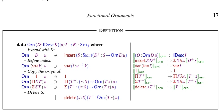
dataOrn(D:IDescK)[u:I→K]:SET1where – Extend with S:

Orn D u 3 insert(S:SET)(D+:S→OrnD u)

– Refine index:

Orn(vark)u 3 var(i:u−1k)

– Copy the original:

Orn 1 u 3 1

Orn(ΠS T)u 3 Π(T+:(s:S)→Orn(T s)u)

Orn(ΣS T)u 3 Σ(T+:(s:S)→Orn(T s)u)

– Delete S:

| delete(s:S)(T+:Orn(T s)u)

J(O:OrnD u)Korn : IDescI JinsertS D

+

Korn 7→ΣSλs.JD

+_s

Korn Jvar(invi)Korn 7→vari

J1Korn 7→1 JΠT

+

Korn 7→ΠSλs.JT

+_s

Korn JΣT

+

Korn 7→ΣSλs.JT

+ sKorn

Jdeletes T

+

Korn 7→JT

+

Korn DEFINITION

Fig. 3: Universe of ornaments

4 A Universe of Ornaments

Originally, McBride (2013) presented the notion of ornament for a universe where the indexing discipline couldonlybe enforced by equality constraints. As a result, the deletion ornament was not expressible in that setting. We shall now adapt the original definition to our system.

4.1 Definition(Universe of ornaments16). The grammar of ornaments (Fig. 3) is similar to the original one. It is defined over a base datatypeDindexed byKand ornaments it to a datatype indexed byI. The (forgetful) functionu:I→Kspecifies a refinement of theK-indices intoI-indices. We cancopythe base datatype (with the codes1,Π, andΣ),extendit by inserting sets (with the codeinsert), and refinethe indexing subject to the relation imposed byu(with the codevar). Also, following Brady’s insight that inductive families need not store their indices(Bradyet al., 2003), we candeleteparts of the datatype definition as long as we can provide a witness. This witness will typically be provided by the index, here in the context.

The extension of ornaments computes the description of the extended datatype. This amounts to travers-ing the ornament code, packtravers-ing the freshlyinsert-ed data intoΣcodes. In thedeletecase, noΣcode is

generated: we use the witness to compute the extension of the rest of the ornament. TheΠandΣornament codes simply duplicate the underlying datatype definition: we retrieve the setSfrom the index ornament D(which is equal toΣS Tfor aΣornament, and toΠS T for aΠornament).

O

4.2 Remark(Inverse image17). The inverse of a function f is defined by the following inductive type

data[f:A→B]−1_{(b:B):SETwhere} f−1(b=f a)3inv(a:A)

DEFINITION

16 _M

ODEL: Orn.Ornament

Equivalently, it can be defined with aΣ-type:

(f:A→B)−1(b:B) : SET

f−1_{b 7→(a:A)×f a=b}

♦

4.3 Definition(Ornament18). An ornament is defined upon a base datatype – specified by a description D:funcK – and a refined set of indices – specified by a function u:I→K. The ornament ofDis an I-familyof ornament codes for eachD(u i), withi:I:

orn(D:funcK) (u:I→K):SET1

ornD u7→(i:I)→Orn(D(u i))u

J(o:ornD u)Korn:funcI JoKorn7→λi.Jo iKorn DEFINITION

In effect, ornamenting a descriptionfuncconsists merely inliftingthe ornamentation ofIDesccodes to a family indexed byI.

O

4.4 Remark(Overloaded notation). We overload the symbol _J−_Korn to denote both the interpretation of an ornament code to a description code (Definition 4.1), and the interpretation of an ornament to a description (Definition 4.3). As for descriptions (Remark 3.4), the latter is merely of pointwise lifting of the former.

♦

4.1 Notation

As for inductive definitions, we adopt an informal notationto succinctly define ornaments. The idea is to simply mirror ourdatadefinition, addingfromwhich datatype the ornament builds upon. When specifying a constructor, we can then extend it with new information – using[x:S]– or delete an argument originally namedxby providing a witness – using [x_,s]. We require the order of constructors to be preserved across ornamentation, as their name might change from the original to the ornamented version. This high-level notation enables us to succinctly specify ornaments. It provides an abstraction over the code of ornament, in the same manner that inductive definitions let us abstract over the code of description (Section 3.3). From the definition of an ornamented typeT, we conventionally callT-Ornits ornament code. A formal description of the translation is beyond the scope of this article. Nonetheless, a few examples are enough to illustrate our notation and shall help us build some intuition for ornaments.

In an effort to reduce the syntactic noise, our notation for ornaments does not specify the forgetful function relating the indices of the ornamented type to its base type. For the examples given in this article, these functions can be inferred from the context. If in doubt, the reader should consult the corresponding definitions in the Agda model. In an actual implementation, the user would have to provide this information.

4.5 Example (Ornament: from Booleans to the option type19_{). We obtain the option type from the} Booleans by inserting an extraa:Ain thetruecase:

dataMaybe[A:SET]fromBoolwhere

MaybeA 3just[a:A] | nothing

Maybe-Orn(A:SET) : orn Bool-func id

Maybe-Orn A 7→λ∗.insert

’just ’nothing

’just 7→delete’true(insertAλ−.1) ’nothing7→delete’false1

We leave it to the reader to verify that the interpretation of this ornament (by J−Korn) followed by the interpretation of the resulting description (by _J−_K) yields the signature functor of the option type X7→1+A:

JJMaybe-OrnAKornKX∼=1+A

4

4.6 Remark(Notation). To reduce the notational burden, we overload the interpretation of ornaments

J−Kornto denote both the description and the interpretation of that description. For instance, we write the above isomorphism as follows:

JMaybe-OrnAKornX∼=1+A

♦

4.7 Example(Ornamenting natural numbers to lists20). We obtain lists from natural numbers with the following ornament:

dataList[A:SET]fromNatwhere

ListA 3nil

| cons[a:A](as:ListA)

List-Orn(A:SET) : orn Nat-func id

List-Orn A 7→λ∗.insert

’nil ’cons

’nil 7→delete’0 1

’cons7→delete’suc(insertAλ−.var(inv∗))

Unfolding the interpretations, we check that we obtain the signature functor of listsX7→1+A×X:

JList-OrnAKornX∼=1+A×X

4

19 _M

ODEL: Orn.Ornament.Examples.Maybe

4.8 Example(Ornamenting natural numbers to finite sets21_{). We obtain finite sets by inserting a number} n0:Nat, constraining the indexntosucn0, and – in the recursive case – indexing atn0:

dataFin(n:Nat)fromNatwhere

Finn3f0[n0:Nat][q:n=sucn0]

| fsuc[n0:Nat][q:n=sucn0](k:Finn0)

Fin-Orn : orn Nat-func(λn.∗)

Fin-Orn7→λn.insert

_’f0

’fsuc



  

  

’f0 7→delete’0

(insertNatλn0.insert(n=sucn0)λ−.1) ’fsuc7→delete’suc

(insertNatλn0.insert(n=sucn0)λ−.var(invn0))



  

  

Again, we leave it as an exercise to unfold the interpretations of this ornament and verify that it is indeed describing the signature of finite sets.

4

4.9 Example(Identity ornament22). In Section 2, we have introduced theidentity ornamentidOas the (trivial) ornament that merely duplicates the definition of its base type. This construction is a straightfor-ward generic program over description codes:

idO(D:IDescI) : OrnDid idO (vari) 7→var(invi)

idO 1 7→1

idO (ΠS T) 7→Πλs.idO(T s) idO (ΣS T) 7→Σλs.idO(T s)

which lifts then pointwise to ornaments:

idO:(D:funcI)→ornDid

4

In Section 3.3, we had to adapt the original presentation of ornaments to our universe. In the process, we have discovered a new ornamental operation, namely the “deletion ornament”. In Section 4.2, we explore some of the possibilities offered by having such a code in our system. However, we shall also verify that the ornamental constructions presented in the original framework still apply: this shall be the topic of Section 4.3 – where we recast theornamental algebrain our setting – and Section 4.4 – where we recast thealgebraic ornamentconstruction. Finally, we revisit thealgebraic ornament by the ornamental algebrain Section 4.5, making crucial use of the deletion ornament and of the optimisations discussed in the following section.

21 _M

ODEL: Orn.Ornament.Examples.Fin

4.2 Brady optimisations, internalised

In Example 3.8, we have seen an example of Brady’s forcing and detagging optimisations, respectively on finite sets and vectors. We have explained how, thanks to our definition of descriptions as functions, we could (manually) craft datatypes in this form. Instead of a presentation based on constraints, we gave an equivalent but less redundant definition. Seen as a datatype transformation, this operation is (obviously) structure-preserving. In fact, these transformations are an instance of ornamentation. The key ingredient is thedeletecode that lets us delete parts of a definition, using a witness extracted from the index. We can therefore craft our own Brady-optimised datatypes by ornamentation and benefit from this optimisation as early as at type checking.

To illustrate this approach, we give an example of detagging (Example 4.10) and forcing (Exam-ple 4.11). To focus solely on the Brady optimisations, we define these ornaments on the naive indexed family we wish to optimise. In practice, we wouldcompose(Dagand & McBride, 2013a) the ornament of natural numbers (Example 1.4 (p.2) for vectors, and Example 4.8 for finite sets) with these optimisations. The composition would directly give the optimised version of, respectively, vectors and finite sets, thus avoiding an unnecessary duplication of isomorphic datatypes.

4.10 Example(Detagging, by ornamentation23_{). The definition of vectors in Example 3.7 mirrors Agda’s} convention of constraining indices with equality. Our definition of ornaments lets us define a version of

Vecthat does not store its indices. Indeed, we can describeVecby an ornament that matches the indexn to determine which constructor to offer:

dataVec’[A:SET](n:Nat)fromVecA nwhere

Vec’A 0 3nil

Vec’A(sucn)3cons[n0_,n](a:A)(vs:Vec’A n)

Vec’-Orn (A:SET) : orn Vec-func id

Vec’-Orn A 0 7→insert{’nil}λ−.delete’nil(deleterefl1)

Vec’-Orn A (sucn)7→insert{’cons}λ−.

delete’cons(deleten(deleterefl(Σλ−.var(invn))))

Such a definition was unavailable in the original presentation of ornaments (McBride, 2013). We have internalised detagging: the constructors of the datatype are determined by the index.

4

4.11 Example(Forcing, by ornamentation24). The definition of finite sets given in Example 3.7 is also subject to an optimisation: by matching the index, we can avoid the duplication ofnby deletingn0with the matched predecessor and trivialising the proofs. Hence,Fincan be further ornamented to the optimised

23 _M

ODEL: Orn.Ornament.Examples.Vec

Fin’, which makes crucial use of deletion:

dataFin’(n:Nat)fromFinnwhere

Fin’ 0 3[b:0] Fin’(sucn)3f0[n0_,n]

| fsuc[n0,n](k:Fin’n0)

Fin’-Orn : orn Fin-func id Fin’-Orn 0 7→insert00-elim

Fin’-Orn(sucn)7→Σ

’f0 7→deleten(deleterefl1)

’fsuc7→deleten(deleterefl(var(invn)))

Note that whennis 0, there is in fact no constructor: we insert the empty set0 to account for the absence of constructor at this index.

Again, this definition was previously unavailable to us. We have internalised forcing: the content of the constructors – heren0– are retrieved from the index, instead of being needlessly duplicated.

4

4.12 Remark(Non-generic transformations). The above transformations aread-hoc: we have to manually give the ornament that performs the detagging and/or forcing. Because of the higher-order nature of our universe of descriptions, we cannot analyse the link between the indices, and the constructor choice and the constructor’s contents. To achieve this from within type theory, we would need a first-order language for describing (a sufficiently expressive fragment of) the function spaceI→IDescI. This is left to future work.

♦

4.3 Ornamental algebra

Every ornament induces anornamental algebra(McBride, 2013): an algebra that forgets the extra infor-mation introduced by the extensions, mapping the ornamented datatype back to its original form.

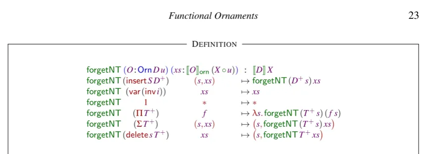
4.13 Definition(Cartesian morphism25). For an ornamentO:OrnD u, there is a function – actually, a natural transformation (Dagand & McBride, 2013a) – projecting the ornamented functor down to the non-ornamented one (Fig. 4). This function then lifts pointwise to ornaments:

forgetNT:(o:ornD u)→JoKorn(X◦u)i→JDKX(u i) DEFINITION

O

forgetNT(O:OrnD u) (xs:JOKorn(X◦u)) : JDKX

forgetNT(insertS D+) (s,xs) 7→forgetNT(D+s)xs forgetNT (var(invi)) xs 7→xs

forgetNT 1 ∗ 7→∗

forgetNT (ΠT+) f 7→λs.forgetNT(T+s) (f s)

forgetNT (ΣT+) (s,xs) 7→ s,forgetNT(T+s)xs forgetNT(deletes T+) xs 7→ s,forgetNTT+xs

DEFINITION

Fig. 4: Cartesian morphism

4.14 Definition (Ornamental algebra26 ). Applied withµDfor X and post-composed with the initial algebrain, this Cartesian morphism induces the ornamental algebra:

forgetAlg(o:ornD u) : JoKorn(µD◦u)i→µD(u i)

forgetAlg o 7→in◦(forgetNTo) DEFINITION

O

4.15 Definition(Forgetful map26 ). In turn, this algebra induces a forgetful map from the ornamented type to its original form:

forget(o:ornD u) : µJoKorni→µD(u i)

forget o 7→_LforgetAlgoM DEFINITION

where_L(α:∀i.JDKX i→X i)M:∀i.µD i→X idenotes the catamorphism, which can be implemented in terms ofinduction(Chapmanet al., 2010).

O

4.16 Example(From lists back to natural numbers27). Applied to the ornamentList-Orn, the Cartesian morphism removes the extra information added through insert, i.e.the inhabitant of A. The resulting algebra thus takesnilto0, andconsatosuc. In turn, the forgetful map computes the length of the list. We have (automatically) constructed thelengthfunction from Section 2.

4

26 _M

ODEL: Orn.Ornament.Algebra

4.17 Example(From the option type back to Booleans28_{). Applied to the ornamentMaybe-Orn, the} Cartesian morphism removes thea:Awe attached to the constructortrue. The forgetful map corresponds exactly to the functionisJust(Section 2).

4

4.18 Example (From finite sets back to natural numbers 29 ). Applied to the ornament Fin-Orn, the Cartesian morphism removes the equations introduced by insert and forgets the indexing discipline enforced by the varcode. The resulting forgetful map computes the cardinality – a natural number – of a finite set. It corresponds to the following function:

forget Fin-Orn(k:Finn) : Nat forget Fin-Orn f0 7→0

forget Fin-Orn (fsuck) 7→suc(forget Fin-Ornk)

4

4.19 Example(From optimised finite sets to na¨ıve finite sets29). When an ornament relies on adelete operation, theforgetfulmap has the – perhaps counter-intuitive – task to re-introduce the deleted informa-tion into the base datatype. To do so, it simply uses the informainforma-tion obtained from the index to fill-in the deleted arguments. For example, the forgetful map obtained fromFin’-Orncorresponds to the following function:

forget Fin’-Orn(n:Nat) (k:Fin’n) : Finn

forget Fin’-Orn (sucn) f0 7→f0nrefl

forget Fin’-Orn (sucn) (fsuck) 7→fsucnrefl(forget Fin’-Ornn k)

where, to be explicit about the origin of the recovered data, we pass the indexnas an explicit argument.

4

4.4 Algebraic ornaments

An important class of datatypes is constructed byalgebraic ornamentationof a base datatype. An alge-braic ornament30 indexes an inductive type by the result of a catamorphism over its elements. From the codeD:funcK and an algebraα:∀k.JDKX k→X k, we define the algebraic ornament, denotedD

α_{, as}

the signature indexed by(k:K)×Xkthat satisfies the following coherence property:

For allk:Kandx:µD k, we have:

µJD

α

Korn(k,x) ∼= (t:µD k)×LαMt=x (4.20) META-THEOREM

Seen as a refinement type, this states that µJD

α

Korn(k,x)is an inductive definition equivalent to the refinement type31{t∈µD k|_Lα_Mt=x}. A categorical presentation is given by Atkeyet al.(2012), who explore the connection between refinement types and inductive families.

28 _{MODEL: Orn.Ornament.Examples.Maybe} 29 _M

ODEL: Orn.Ornament.Examples.Fin

30 _M

ODEL: Orn.AlgebraicOrnament

The type-theoretic construction ofDα_{was originally given by McBride (2013). We shall not reiterate}

it here, the implementation being essentially the same.The idea is to define – by ornamentation ofD– a description whose fixpoint will satisfy the above coherence property.

4.21 Remark(Computational interpretation). Constructively, the coherence property (4.20) gives us two (mutually inverse) functions,coherentOrnandmakeDα_.

The directionµJD

α

Korn(k,x)→(t:µD k)×LαMt=xrelies on the generic forgetful mapforgetD

α _to

compute the first component of the pair and gives us the following theorem32:

coherentOrn:(t+:µJD

α

Korn(k,x))→LαM(forgetD

α_t+_)=x DEFINITION

This corresponds to theRecomputationtheorem of McBride (2013). We shall not reprove it here, the construction being similar.

In the other direction, the isomorphism (4.20) gives us a function of type

(t:µD k)×LαMt=x→µJD

α

Korn(k,x)

which, after simplifying the equation, gives a function that lifts a datatype to its algebraic version33, at the index computed by the predicate:

make(D:funcI)(α:∀i.JDKX i→X i)_:(t:

µD k)→µJD

α

Korn(k,LαMt) DEFINITION

This corresponds to therememberfunction of McBride (2013). Again, we will assume this construction here.

♦

4.22 Example(Algebraic ornament: vectors). Ornamenting natural numbers to lists, we obtain an orna-mental algebra: the algebra computing the length of a list. We can therefore build the algebraic ornament of lists by the length algebra34_{. This correspondsexactlyto the datatype of vectors (Example 3.7): the} resulting signatures are isomorphic, and both rely on constraints to enforce the indexing discipline.

Note that this operation generalises to all ornaments: any ornament induces an ornamental algebra. Therefore, we can always build the algebraic ornament by the ornamental algebra. We shall study this operation in more details in Section 4.5.

4

32 _M

ODEL: Orn.AlgebraicOrnament.Coherence

33 _M

ODEL: Orn.AlgebraicOrnament.Make

4.23 Example(Algebraic ornament: less-than-or-equal relation35). For a given natural numberm:Nat, the additionm+−:Nat→Natis obtained by folding the algebra

plusAlg(m:Nat) (xs:JNat-funcKNat∗) : Nat

plusAlg m (’0,∗) 7→m

plusAlg m (’suc,n) 7→sucn

By algebraically ornamentingNatby this algebra, we obtain the relationm≤−:Nat→SET that is characterised by the isomorphism

m≤n ∼= (k:Nat)×m+k=n

Put explicitly, the datatype computed by the algebraic ornament corresponds to

data[m:Nat]≤(n:Nat):SETwhere

m≤(n=m) 30

m≤(n=sucn0) 3suc(k:m≤n0)

4

4.24 Example(Algebraic ornament: indexing by semantics36_{). A typical use-case of algebraic ornaments} is the implementation of semantic-preserving operations (McBride, 2013). For example, let us consider arithmetic expressions, whose semantics is given by interpretation toNat:

dataExpr:SETwhere

Expr 3const(n:Nat) | add(d:Expr)(e:Expr)

evalAlg(es:_JExpr-func_KNat∗) : Nat evalAlg (’const,n) 7→n

evalAlg (’add,(m,n)) 7→m+n

Using the algebraevalAlg, we construct the algebraic ornament ofExprand obtain expressions indexed by their semantics:

dataExprevalAlg(k:Nat):SETwhere

ExprevalAlg (k=n) 3const(n:Nat)

ExprevalAlg(k=m+n)3add(m n:Nat)(d:ExprevalAlgm)(e:ExprevalAlgn)

We can now enforce the preservation of semantics by typing. For example, let us optimise away all additions of the form “0+e”:

optimise-0+ (e:ExprevalAlgn) : ExprevalAlgn

optimise-0+ (constn) 7→constn

optimise-0+ (add 0n d e) 7→optimise-0+e

optimise-0+(add(sucm)n d e)7→add(sucm)n d e

Because the type checker accepts our definition, we have that, by construction, this operation preserves the semantics. We can then prune the semantics from the types using the forgetful map and retrieve the transformation on raw syntax trees. Themake function (Remark 4.21) lets us lift raw syntax trees to semantically-indexed ones, while thecoherentOrntheorem (Remark 4.21) certifies that the pruned tree satisfies the invariant we enforced by indexing.

4

35 _M

ODEL: Orn.AlgebraicOrnament.Examples.Leq

4.5 Reornaments

In this article, we are particularly interested in a sub-class of algebraic ornaments. In Definition 4.14, we have constructed, for an ornament o, its ornamental algebraforgetAlgo that forgets the extra in-formation introduced by the ornament. As hinted at in Example 4.22, given an ornament o, we can always algebraically ornament _Jo_Korn using the ornamental algebra forgetAlgo. McBride (2013) calls this construction thealgebraic ornament by the ornamental algebra.

4.25 Remark(Notation). We writedoeto denote the algebraic ornament ofoby the ornamental algebra. For brevity, we call it thereornamentofo.

♦

4.26 Example(Reornament: vectors). Paraphrasing Example 4.22, we have that vectors are a reornament ofList-Orn. Explicitly, a vector is the algebraic ornament ofListby the algebra computing its length,i.e. the ornamental algebra fromListtoNat.

4

4.27 Example (Reornament: indexed option type). In Example 4.5, we ornamented Booleans to the option type. We can thus reornament the option type with its Boolean status. Unfolding the definition of the reornament, we obtain the IMaybeA datatype that was introduced in Section 2. The function

forgetIMaybecorresponds to the left-to-right reading of the isomorphism (4.20) specialised to theMaybe

ornament.

4

Reornaments are thus straightforwardly obtained through a two steps process: first, compute the orna-mental algebra and, second, construct the algebraic ornament by this algebra. However, such a simplistic construction introduces a lot of spurious equality constraints and duplication of information. For instance, using this naive definition of reornaments, a vector indexed bynis constructed asanylistas long asit is of lengthn.

4.28 Example(Reornamenting vectors, efficiently). Let us consider the ornamentList-Orn, taking natu-ral numbers to lists. We gave its code in Example 4.7. Here, for simplicity, we shall work on the following variant

List-Orn(A:SET) : orn Nat-func id

List-Orn A 7→λ∗.Σ

’0 7→1

’suc7→insertAλ−.var(inv∗)

which does not update the constructor names, allowing us to focus on the essential transformations. We can adopt a more fine-grained approach yielding an isomorphic but better structured datatype. In our setting, where we can compute over the index, a finer construction of the reornament ofList-Ornis as follows:

• We retrieve the index, hence obtaining a numbern:Nat;

• By inspecting the ornamentList-Orn, we obtain theexactrelationship between the indexnand its ornament describing lists

• Ifn=0, we are in the first branch of theΣcode, and the ornamentation of nis necessarily the

empty list. The corresponding reornament can therefore delete the choice of constructor (since it is entirely determined by the index), set it to’0, and terminate immediately:

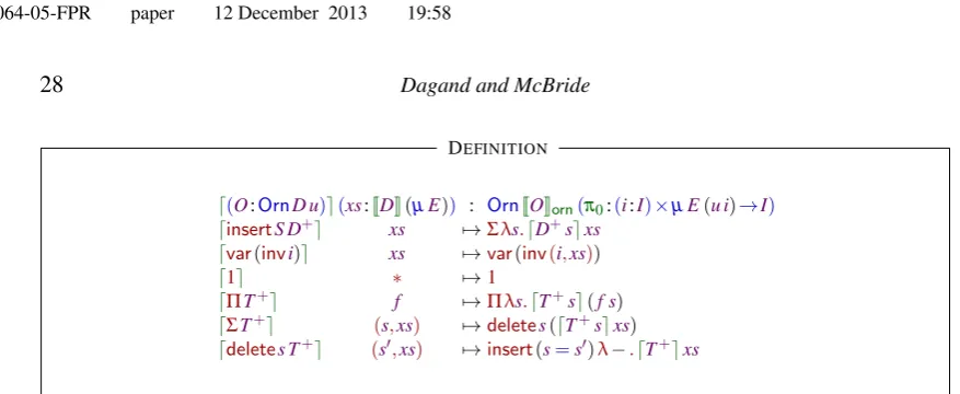
d(O:OrnD u)e(xs:JDK(µE)) : OrnJOKorn(π0:(i:I)×µE(u i)→I) dinsertS D+e xs 7→Σλs.dD+sexs

dvar(invi)e xs 7→var(inv(i,xs))

d1e ∗ 7→1

dΠT+e f 7→Πλs.dT+se(f s) dΣT+e (s,xs) 7→deletes(dT+_sexs) ddeletes T+e (s0,xs) 7→insert(s=s0)λ−.dT+_exs

DEFINITION

Fig. 5: Reornament

• Ifn=sucn0, we are in the second branch of theΣcode, and the ornament ofsucn0is a necessarily

non-empty list. Again, the corresponding reornament deletes the choice of constructor, by deducing from the index that it must be ’cons. Since the list ornament extends natural numbers with an argument of typeA(through theinsertcode), we must preserve this information in the reornament (through aΣcode). Finally, we index the recursive argument of the reornamented datatype byn0:

dList-OrnA∗e ’suc,n0 delete’suc(Σλa.var(inv ∗,n0))

Altogether, we have ornamented lists by their length: when the index is0, the ornamented list is empty; when the index issucn0, the ornamented list is non-empty and takes an argument indexed byn0. We have effectively described the datatype of vectors.

4

4.29 Definition(Reornament37_{). A reornament (Fig. 5) is thus defined over an ornament codeO:OrnD u} (for some descriptionD:IDescI) and an index belonging to the base datatypexs:_JD_K(µD). On the1 andΠcodes, the reornament simply mirrors the underlying ornament, while peeling off the index: the

structureof the three datatypes is identical. On avarcode, the reornament also duplicates the underlying structure by pairing the index of the ornament (provided by the indexi) with the recursive argument of the base datatype (provided by the argumentxs). On aninsertcode, the reornament preserves the extra-information introduced by the ornament since it is absent from the index. However, on aΣcode, the

ornament is merely duplicating information already provided byxs: in this case, we delete the argument, filling in the gap with the data provided by the indexxs. On adeletecode, we make sure – through an equality constraint – that the indexxsis in sync with the data deleted by the ornament.

This definition over codes then lifts pointwise to ornaments:

d(o:ornD u)e : orn_Jo_Korn(π0:(i:I)×µD(u i)→I)

doe 7→λ(i,inxs).do iexs

DEFINITION

O

4.30 Example(Reornament: vectors38_{). Applied to the ornamentList-Orn(Example 4.7), this} construc-tion gives the fully Brady-optimised – detagged and forced – version of vectors (Example 3.8). That is, we determine which constructor ofVecis available by pattern-matching on the index. This is unlike the naive reornament (Example 4.26), which relies on constraints to enforce the indexing discipline.

4

4.31 Example(Reornament: indexed option type39). Under this definition, the reornament ofMaybe-Orn

(Example 4.5) describes the datatype

dataIMaybe[A:SET](b:Bool):SETwhere

IMaybeAtrue3just(a:A) IMaybeAfalse3nothing

where, similarly, constraints are off-loaded by pattern-matching on the indices (Example 3.8). Again, this must be compared with the definition obtained through the naive construction (Example 4.27), where we relied on constraints.

4

Note that our ability tocomputeover indices is crucial for this construction to work. Also, the datatypes we obtain are isomorphic to the datatypes one would have obtained by the algebraic ornament of the ornamental algebra,i.e.:

For all ornamento:ornD u, we have

JdoeKorn ∼= JJoKorn forgetAlgo

Korn META-THEOREM

4.32 Remark(Computational interpretation). Consequently, the coherence property of algebraic orna-ments (Equation 4.20) is still valid. Constructively, this isomorphism gives thecoherentOrntheorem40in one direction and themake function41in the other.

♦

4.33 Remark (Iterating reornamentation42). Every ornament induces a reornament. A reornament is itself an ornament: it therefore induces yet another reornament. We are naturally led to wonder if this process ever stops, and if so when. For example, the ornament of natural numbers into lists reornaments to vectors. Reornamenting vectors, we obtain an inductive predicate representing the length function

Length:Nat→ListA→SET. ReornamentingLengthleads to an object with no computational content: all its information has been erased and is provided by the indices.

The same pattern arises in general: every chain of reornaments is bound to end with a computationally trivial object. We deduce this from our massaged definition of reornaments (Definition 4.29). To illus-trate our reasoning, we simultaneously iterate the reornamentation of the following (artificial) ornament

38 _M

ODEL: Orn.Reornament.Examples.List

39 _{MODEL: Orn.Reornament.Examples.Maybe} 40 _M

ODEL: Orn.Reornament.Coherence

41 _M

ODEL: Orn.Reornament.Make

indexed byn:Nat

o : ornD(λn.∗)

o7→λn.Σλa.insertCλc.Πλb.delete true(var(sucn))

which ornaments the description

D : func1

D7→λ∗.ΣAλa.ΠBλb.ΣBoolλx.var∗

whereA,B, andCare sets.

We proceed by case analysis on the ornament. On a1,Π, andvarcode, the reornamentation proceeds

purely structurally, merely duplicating the ornament’s code and introducing no information (Defini-tion 4.29, first 3 cases). The reornamenta(Defini-tiondeletesΣcodes, using the indexing information (Defini-tion 4.29, fourth case). On adeletecode, the reornament inserts an equality constraint (Definition 4.29, sixth case), which contains no information per se: it is only enforcing the indexing discipline. Only on an insertcode does the reornament introduce new information through aΣcode (Definition 4.29, fifth case).

On our example, the first reornament is defined by

o+ : orn(_Jo_Korn:funcNat)π0 o+7→doe

and unfolds to

o+ λ(n,in(a,f)).deletea(ΣCλc.Πλb.insert(true=π0(f b))λ−.var(inv(sucn,π1(f b))))

In the subsequent iteration, theseΣcodes in the reornament are in turn deleted by the re-reornament.

On our example, the second reornamentation is defined by

o++ : orn(_Jo+Korn:Nat×µD∗)π0 o++ 7→do+_e

and unfolds to

o++ λ((n,in(a,f)),in(a0,(c,f+))).insert(a0=a)λ−.deletec(Πλb.Σλq.

var(inv((sucn,π1(f b)),f+b))

where theΣcode duplicates the (computationally trivial) equation onx(true=x) that was inserted in the

previous step.

In the third iteration, there is nothing left in the code but equations and structural scaffoldings (in the form ofvar,1, andΠcodes): the resulting datatype is computationally trivial and is entirely determined

by its indices. On our example, the third reornamentation is defined by

o+++ : orn(_Jo++Korn:func(n:Nat)×µD∗×µJoKornn)π0 o+++7→do++_e

and unfolds to

o+++ λ(((n,in(a,f)),in(a,(c,f+))),in(c0,f++)).

Σλq1.insert(c0=c)λq2.Πλb.deleterefl(var(inv(((sucn,π1(f b)),f+b),π1(f++b))))

where theΣcode duplicates the (computationally trivial) equation ona(a0=a) that was inserted in the