Dimensional analysis of yielding and pounding structures for records without distinct pulses

City, University of London Institutional Repository

Citation

:

10.1016/j.soildyn.2009.02.006

This is the accepted version of the paper.

This version of the publication may differ from the final published

version.

Permanent repository link:

Link to published version

:

Copyright and reuse:

City Research Online aims to make research

outputs of City, University of London available to a wider audience.

Copyright and Moral Rights remain with the author(s) and/or copyright

holders. URLs from City Research Online may be freely distributed and

linked to.

City Research Online: http://openaccess.city.ac.uk/ [email protected]

Dimensional Analysis of Yielding and

Pounding Structures for Records Without

Distinct Pulses

Elias Dimitrakopoulos,1 _{Andreas J. Kappos}2 _{and Nicos Makris}3 Abstract

The seismic response of two fundamental mechanical configurations of earthquake engineering,

the elastic-plastic system and the pounding oscillator, is revisited with the aid of dimensional

analysis. Starting from the previous work of the authors which focused on pulse-type

excitations, the paper offers an alternative, yet physically motivated, way to present the

response of yielding and pounding structures under excitations with arbitrary time-history. It is

shown, that when the appropriate time and length scales are adopted, dimensional analysis can

be implemented and remarkable order emerges in the response. Regardless of the acceleration

level and frequency content of the excitation, all response spectra become self-similar and when

expressed in dimensionless terms, resulting from dimensional analysis, follow a single master

curve. The study proposes such scales together with the associated selection criteria among the

available in literature strong ground motion parameters and shows that the proposed approach

reduces drastically the scatter in the response.

Keywords: Non-linear Structural Dynamics, Dimensional Analysis, Physical Similarity, Earthquake Engineering

1_{Doctoral Candidate, Dept. of Civil Engineering, Aristotle University of Thessaloniki, Greece,}

GR 54124

2_{Professor, Dept. of Civil Engineering, Aristotle University of Thessaloniki, Greece, GR 54124} 3_{Professor, Dept. of Civil Engineering, University of Patras, Greece, GR 26500}

1. INTRODUCTION

A major challenge in studying the response of structures with non-linear behaviour, is no

and presentation of the response analysis in a way that is most meaningful for a broad class of

structural configurations. This challenge emerged partly due to: (1) the ability of modern

computers to rapidly produce a large number of nonlinear solutions, (2) an ever increasing

database of recorded ground motions with quite complex patterns, and (3) the wide scatter in

the structural response calculated from time-history analysis using historic records.

In an effort to partly address this challenge Makris and Black [1, 2] revisited the inelastic

response of elastic-plastic and bilinear systems with the aid of dimensional analysis [3-5] and

subsequently demonstrated the applicability and promise of the proposed approach to various

structural frames known in the literature [5]. More recently, the response of pounding

oscillators, both elastic and inelastic, was also revisited with formal dimensional analysis by

Dimitrakopoulos et al. [6, 7]. In these studies it was shown that the non-linear response of

yielding, as well as pounding, structures, under pulse-type excitations, becomes self-similar

when expressed in the appropriate dimensionless Π-terms derived from formal dimensional

analysis. Self-similarity is a special type of symmetry which is invariant with respect to scale

transformations and it is of unique importance when ordering non-linear behaviour. It is

interesting to note, that self-similarity prevails even when the two non-linearities, the inelastic

behaviour of the structure and the boundary non-linearity of the pounding phenomenon, coexist

[6].

The implementation of dimensional analysis, in the aforementioned studies of Makris et al.

[1, 2, 5] and Dimitrakopoulos et al. [6, 7], hinges upon the existence of a distinct time-scale and

a length scale that characterize the most energetic component of the ground shaking. In the case

of records with distinct pulses, these scales emerge naturally from the acceleration amplitude,

αp, and the duration of the pulse, Tp, and can be formally extracted with validated mathematical

models available in the literature e.g. [8]. The aforementioned studies brought forward the

coined by Makris [1], which liberates the non-linear response from the need to refer to a

'substitute' system (e.g. the elastic SDOF oscillator) and reveals the property of self-similarity in

the response.

The aforementioned work of the authors on the dimensional analysis of non-linear systems

was justified by the distinct coherent pulses identified in a wide class of strong motion records,

mostly near source ones. The present study is motivated by the need to extend the application of

the dimensional analysis approach for excitations without distinct pulses, as well as to

contribute to the goals of the work of Kappos & Kyriakakis [9] who re-evaluated the problem of

reducing the scatter in the structural response to natural records.

2. TIME AND LENGTH SCALES IN EARTHQUAKE RECORDS WITH DISTINCT PULSES

The present section builds on the work of several researchers [8, 10, 11] who adopted

typical pulses in order to simulate (the long period component of) real earthquake excitations.

During the last three decades, an ever-increasing database of recorded ground motions has

shown that the kinematic characteristics of the ground motion near the fault of major

earthquakes contains distinguishable acceleration and velocity pulses (e.g. Figure 1). The

relatively simple form and the destructive potential of near source ground motions have

motivated the development of various closed-form expressions which approximate their leading

kinematic characteristics. Physically realizable trigonometric pulses can adequately describe the

impulsive character of near-fault ground motions both qualitatively and quantitatively.

Figure 1 plots the acceleration, Ag, velocity, Vg, and displacement, Dg, time-histories of the

NS record, from the 1992 Erzincan earthquake . It is clear that: a) the main characteristics of the

record can be captured with the use of a simple pulse, and b) that the period of the distinct

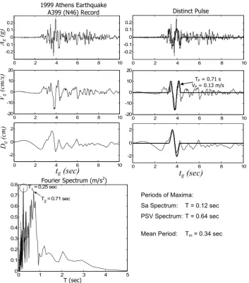
time-histories and the Fourier spectrum of the A399 record from the Athens 1999 earthquake.

Unlike the Erzinzan record, the period of the distinct pulse does not correspond to the peak of

the Fourier amplitude spectrum, yet it is still distinguishable in it.

0 2 4 6 8 10

-0.5 0 0.5

0 2 4 6 8 10

-100 0 100

0 2 4 6 8 10

-40 -20 0 20 40

0 2 4 6 8 10

-0.5 0 0.5

0 2 4 6 8 10

-100 0 100

0 2 4 6 8 10

-40 -20 0 20 40

1992 Erzincan Earthquake (NS)

A

(g

)

V

(cm

/s)

D

(c

m

)

Distinct Pulse

Fourier Spectrum (m/s2₎

Τ (sec)

Periods of Maxima: Sa Spectrum: Τ = 0.3 sec PSV Spectrum: Τ = 2.04 sec

Mean Period: Tm = 1.33 sec

t

(sec)

t

(sec)

0 1 2 3 4 5

0 0.5 1 1.5 2 2.5 3

T₁ = 2.0 sec

Τp = 2.0 s vp = 0.56 m/s

Figure 1: Top left: acceleration, Ag, velocity, Vg, and displacement, Dg, time-histories of the Erzincan (NS) earthquake record. Top right: the distinct pulse. Bottom: the Fourier

0 2 4 6 8 10 -0.2

-0.1 0 0.1 0.2

0 2 4 6 8 10

-20 -10 0 10 20

g

0 2 4 6 8 10

-2 0 2

g

t_g (sec)

0 2 4 6 8 10

-0.2 -0.1 0 0.1 0.2

0 2 4 6 8 10

-20 -10 0 10 20

0 2 4 6 8 10

-2 0 2

t_g (sec)

TP = 0.71 s

VP = 0.13 m/s

Ag

(g)

Vg

(cm/s)

Dg

(cm)

1999 Athens Earthquake

Α399 (Ν46) Record Distinct Pulse

Τ (sec)

Fourier Spectrum (m/s2₎

Periods of Maxima:

Sa Spectrum: Τ = 0.12 sec PSV Spectrum: Τ = 0.64 sec

Mean Period: Tm = 0.34 sec

t

(sec)

t

(sec)

Τ (sec)

0 1 2 3 4 5

0 0.1 0.2 0.3 0.4 0.5 0.6 0.7 0.8 _T

1 = 0.25 sec

T₂ = 0.71 sec

Figure 2: Top left: acceleration, Ag, velocity, Vg, and displacement, Dg, time-histories of the A399 (N46) record. Top right: the distinct pulse. Bottom: the Fourier amplitude

spectrum.

Figure 3 presents the Newhall station record, from the 1994 Northridge earthquake. At least

four of the non high-frequency peaks of the Fourier spectrum (Τ1 = 0.59 sec, Τ2 = 0.71 sec, Τ3 =

1994 Northridge Earthquake Newhall Station (FP)

0 2 4 6 8 10

-1 -0.5 0 0.5 1

0 2 4 6 8 10

-100 -50 0 50 100 150

0 2 4 6 8 10

-40 -20 0 20

0 2 4 6 8 10

-1 -0.5 0 0.5 1

0 2 4 6 8 10

-100 -50 0 50 100 150

0 2 4 6 8 10

-40 -20 0 20

0 1 2 3 4 5

0 1 2 3 4 5

T₁ = 0.59 sec

T₂= 0.71 sec

T₃= 1.3 sec

T₄= 2.0 sec

A

(g)

V

(cm/s

)

D

(cm)

Τp3 = 1.3 s vp3 = 0.8 m/s

Τp2 = 0.7 s vp2 = 0.9 m/s

Τp4 = 2.0 s vp4 = 0.4 m/s

Τp1 = 0.6 s vp1 = 0.3 m/s

Fourier Spectrum (m/s2₎

Τ (sec)

Periods of Maxima:

Sa Spectrum: Τ = 0.66 sec PSV Spectrum: Τ = 0.72 sec

Mean Period: Tm = 0.67 sec

t

(sec)

t

(sec)

Figure 3: Top left: acceleration, Ag, velocity, Vg, and displacement, Dg, time-histories of the Newhall station record. Top right: the distinct pulse. Bottom: the Fourier amplitude

spectrum.

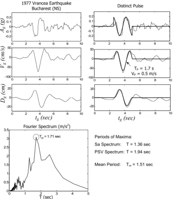
Distinct pulses appear usually, but not always [12, 13], in near-source ground motions

(Figure 1). On the other hand, there exist far-field records that contain also distinguishable

pulses; a typical example is the Bucharest record of the 1977 Vrancea earthquake (Figure 4)

where the presence of a deposit filtered/amplified an earthquake signal which originated more

0 2 4 6 8 10 -0.2

-0.1 0 0.1 0.2

0 2 4 6 8 10

-100 -50 0 50

0 2 4 6 8 10

-20 0 20

T_P=1.7 sec

v_P=0.5 m/s

0 2 4 6 8 10

-0.2 -0.1 0 0.1 0.2

g

0 2 4 6 8 10

-100 -50 0 50

g

0 2 4 6 8 10

-20 0 20

1977 Vrancea Earthquake

Bucharest (NS) Distinct Pulse

Τ (sec) Fourier Spectrum (m/s2₎

Periods of Maxima:

Sa Spectrum: Τ = 1.36 sec PSV Spectrum: Τ = 1.94 sec

Mean Period: Tm = 1.51 sec

A

(g

)

V

(cm

/s

)

D

(cm)

t

(sec)

t

(sec)

0 1 2 3 4 5

0 0.5 1 1.5 2 2.5 3 3.5

T_P = 1.71 sec

TP = 1.7 s

VP = 0.5 m/s

Figure 4: Top left: acceleration, Ag, velocity, Vg, and displacement, Dg, time-histories of the Bucharest (NS) record. Top right: the distinct pulse. Bottom: the Fourier amplitude

spectrum.

The present analysis confirms that in the case of records with distinct pulses, the period of

these pulses in general corresponds to visible peaks in the associated Fourier spectrum. Thus,

the Fourier spectrum can be exploited in order to identify the time-scale of such excitations,

observation is in agreement with the model of Mavroeidis & Papageorgiou [8], according to

which the (time-scale) ‘duration of the pulse’, Tp, is considered as Tp = 1/ fp, where fp is the

predominant frequency of the signal. It is recalled that, even though the duration of a pulse

usually coincides with its predominant period, the two notions ‘duration’ and ‘period’, are

differentiated for excitations with more than one loading cycle.

To summarize, for records with (one or more) distinct pulses, it is usually feasible to

identify the period of the non high-frequency pulses in the pertinent Fourier spectrum. This

observation brings forward the essential time-scale of an excitation when a peak response

parameter is of interest, i.e. its frequency content, and paves the way for the generalization of

the dimensional response analysis approach, for records without distinct pulses.

3. TIME AND LENGTH SCALES IN EARTHQUAKE RECORDS WITHOUT DISTINCT PULSES

Several challenges emerge when trying to generalize the concept of using typical pulses in order

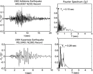
to simulate a real record. First of all, in many records there is no distinct pulse, but rather their

form is composed of random acceleration spikes (Figure 5). On the other hand, even when a

record contains more than one distinguishable pulse, it is not clear how to incorporate the

characteristics of those pulses into a single time-scale (or parameter). Hence arises the need to

characterize a record with a time-scale directly, without comparing it with one or more typical

pulses.

The present paper proposes the use of appropriate strong ground-motion parameters, already

available in the literature, which allow the implementation of the dimensional-analysis approach

in the case of records with arbitrary shape. Building on the previous work on the dimensional

response analysis of structures [1, 2, 6, 7] the desired properties, of the appropriate time and

0 2 4 6 8 10 -0.2

-0.1 0 0.1 0.2

a g

(g

)

t (sec)

1984 ΣεισμοςΚυπαρισσίας Καταγραφή PEL18401 N(280)

0 1 2 3 4 5

0 0.2 0.4 0.6 0.8 1

T (sec) T₁ = 0.15 sec

Ag

(g

)

0 1 2 3 4 5

0 0.2 0.4 0.6 0.8 1

T (sec) T₁ = 0.28 sec

Fourier Spectrum

(g)

0 5 10 15 20

-0.2 -0.1 0 0.1 0.2

ag

(g)

t (sec) 1983 ΣεισμόςΚεφαλονιάς Καταγραφή ARG18307 N(59)

Ag

(g

)

1984 Kyparissia Earthquake PEL18401 N(280) Record 1983 Kefalonia Earthquake

ARG18307 N(59) Record

Figure 5 : Left: Acceleration time-histories of typical (Greek) records without distinct pulse. Right: the pertinent Fourier amplitute spectra

3.1 Criteria for Selection of the Strong Ground Motion Parameters

1. The appropriate strong ground motion parameters should be independent of the

structural response. This is essential, since in order to reveal the property of self-similarity, the

non-linear response must be liberated from the need to refer to a ‘substitute system’ (such as an

equivalent linear-elastic system). This was illustrated for both yielding [1, 2] and pounding [6,

7] structures.

2. Given that the response function has to be dimensionally homogeneous, two reference

dimensions are needed, that of time [T] and length [L]. By analogy to the time and length scales

dimensions of time, and one length-scale with dimensions of velocity or acceleration. Hence, a

pair of parameters with appropriate dimensions is requested, such that all involved quantities

can be scaled with the same two parameters and not with a single one.

3. For practical reasons, it is convenient to use a length scale/parameter that is linearly

dependent on the amplitude of the excitation.

4. If feasible, the adopted parameters should have an unambiguous physical meaning and

be easily estimated.

3.2 Proposed Strong Ground Motion Parameters

The aforementioned desired properties, comprise the criteria based on which the appropriate

strong ground motion parameters (one time-scale and one length-scale) can be selected among

the available relevant parameters in the literature.

Hancock & Bommer, after reviewing the pertinent literature [15], and evaluating the results

of an analytical study [16], confirmed that the duration of an excitation has no influence when a

peak response quantity is of interest, like the maximum response displacement, velocity or

acceleration. Hancock & Bommer’s recent conclusions regarding the duration of an excitation,

are in agreement with earlier findings by Kappos [17]. Since the present study focuses on peak

response parameters, the appropriate time-scale should describe the frequency content of the

excitation, not its duration. Mylonakis & Voyagaki [18] considered pulse-type excitations and

showed that the maximum ductility of an inelastic oscillator is much more sensitive to the

time-history shape of an excitation than to the number of loading cycles (of the same excitation).

The period corresponding to the peak acceleration of the elastic response spectrum, TPSA, is

probably the most extensively used frequency parameter in earthquake engineering. Yet, it is

well known that two acceleration spectra with the same TPSA may differ substantially in shape

[19]. Similarly, the period of the peak velocity of the elastic response spectrum, TPSV, is known

However, TPSA, TPSV, as well as the period of any other peak spectral quantity, are (structural)

response-dependent parameters and hence are not considered further herein, since they

contradict the first selection criterion in section 3.1.

On the contrary, the period of the maximum Fourier amplitude spectrum is not dependent

on the structural response. It is well known though, that the Fourier amplitude spectrum may

exhibit a peak at high-frequencies, while the most energetic components of the excitation

correspond to lower frequencies (see e.g. Figure 2). A simple frequency parameter that

overcomes this shortcoming and encloses information about the shape of the Fourier spectrum

is the mean period, Tm, proposed by Rathje et al. [19]. The mean period, Tm, averages the

periods of the Fourier spectrum according to the equation:

2

2 1

i

i i

m

i i

C f T

C







where Ci are the Fourier amplitudes of the accelerogram and fi the discrete Fourier transform

frequencies between 0.25 and 20 Hz. The mean period is known to perform equally well as the

smoothed spectral predominant period [19]. Unlike the pertinent spectral periods, Tm does not

engage structural response and hence complies with the first desired property.

Concerning the appropriate length-scale, the spectral intensity, SI, either in the original

form proposed by Housner [21] or in the modified one proposed by Kappos [17, 22] is an

effective strong ground-motion parameter that has been extensively used by many researchers

[9, 23]. However, SI, is also a response-dependent parameter like the TPSA, TPSV and for the same

reason will not be further considered.

Kappos & Kyriakakis [9] re-evaluated the ability of the most commonly used scaling

parameters to reduce the scatter in the analytically estimated structural response. They

concluded that the acceleration-based parameters, such as the peak ground acceleration, PGA,

period structures, in contrast to velocity-based parameters, such as the peak ground velocity,

PGV, the spectrum intensity, SΙ, and the Fajfar [24] index, Iv, that describe better the response

of intermediate and long period structures. The conclusions of Kappos & Kyriakakis [9] were

further confirmed by the comparative study of an even wider set of strong ground motion

parameters conducted by Riddell [25]. Moreover, Makris & Black [26] considered both linear

and non-linear structural responses under pulse-type excitations and concluded for the set of

records that they examined that PGΑ is a more representative intensity measure than the PGV of

the earthquake shaking.

Another interesting strong ground motion parameter is the cumulative absolute velocity,

CAV, which equals the area under the (absolute) acceleration versus duration curve.

Equivalently, it can be considered as the sum of the consecutive peak-to-valley distances in the

velocity time-history. Thus, CAV condenses information for the amplitude and the duration of

motion and has been known to express the destructive potential of the excitation [27]. The

disadvantage of cumulative parameters like CAV is their dependency on the duration of the

excitation regarding which there is still great uncertainty [15].

Also, more complex parameters like the Fajfar index, Iv, or those examined in references

[28, 29] are not considered herein, either because their dimensions are not the sought ones, or

because they do not comprise a pair of parameters (2nd _{desired property).}

Based on the preceding discussion, the peak ground acceleration, PGA, and the mean

period, Tm, [19] are proposed as the appropriate length and time scales, respectively, of an

excitation with arbitrary time-history shape.

3.3 Selected Ground Motions from Previous Earthquakes

The ground motions used in the present study comprise most of the available historic Greek

records with PGA of 0.1g or more [30]. It is reminded that in Greece all types of faults coexist

the records examined. Table 1 lists these records together with their pertinent characteristics; R

stands for the epicentral distance and fc for the cut-off frequency.

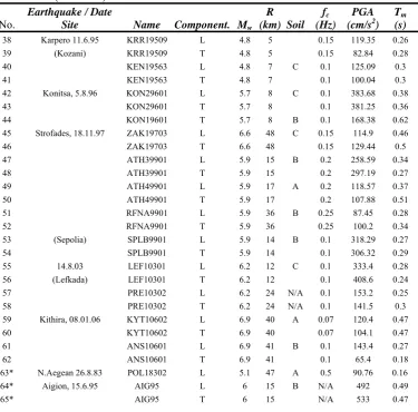
Table 1: Main characteristics of Greek records used [29]

No. Earthquake / Date Site Name Component. Mw R (km) Soil

fc (Hz)

PGA (cm/s2)

Tm (s)

1* Volvi, 20.6.78 THEA7802 L 6.5 26 C 0.2 142.56 0.5

2* (Thessaloniki) THEA7802 T 6.5 26 0.2 146.94 0.47

3* Alkyonides, 24.2.81 KORA8101 L 6.7 32 C 0.15 229.5 0.68

4* (Corinth) KORA8101 T 6.7 32 0.15 274.41 0.55

5* Kefalonia, 17.1.83 ARG18301 L 7 35 B 0.25 173.31 0.26

6* (Argostoli) ARG18301 T 7 35 0.25 142.5 0.33

7* Kefalonia, 23.3.83 ARG18307 L 6.2 26 0.25 179.81 0.2

8* (Argostoli) ARG18307 T 6.2 26 0.25 219.2 0.23

9* Kyparissia, 25.10.84 PEL18401 L 5 9 A 0.2 166.63 0.29

10* (Pelekanada) PEL18401 T 5 9 0.2 172.75 0.31

11* Kalamata, 13.9.86 KAL18601 L 6 12 B 0.1 229.26 0.6

12* (Kalamata) KAL18601 T 6 12 0.1 263.88 0.53

13 Kalamata, 15.9.86 KAL18608 L 5.3 3 0.15 232.79 0.51

14 (Kalamata) KAL18608 T 5.3 3 0.15 137.11 0.46

15 KAL28602 T 5.3 3 0.1 254.31 0.55

16 Zakynthos, 16.10.88 ZAK18804 L 6 20 C 0.2 133.02 0.42

17 ZAK18804 T 6 20 0.2 147.23 0.4

18 AMAA8805 L 6 28 C 0.2 84.11 0.4

19 AMAA8805 T 6 28 0.2 163.62 0.4

20* Griva, 21.12.90 EDE19001 L 6 32 C 0.2 100.13 0.57

21* (Edessa) EDE19001 T 6 32 0.2 94.35 0.59

22 26.3.93 PYR19306 L 4.9 6 C 0.25 105.64 0.21

23 PYR19306 T 4.9 6 0.25 221.48 0.18

24* Vartholomio, 26.3.93 PYR19308 L 5.4 14 0.2 162.86 0.28

25* (Pyrgos) PYR19308 T 5.4 14 0.2 425.85 0.33

26 14.7.93 PAT19302 L 5.6 10 C 0.2 143.74 0.3

27 PAT19302 T 5.6 10 0.2 192.49 0.36

28 PAT29302 L 5.6 9 C 0.25 164.2 0.3

29 PAT29302 T 5.6 9 0.25 388.57 0.22

30* Mt.Vourinos, 13.5.95 KOZ19501 L 6.6 16 A 0.25 211.73 0.27

31* (Kozani) KOZ19501 T 6.6 16 0.25 137.38 0.26

32 Kozani, 15.5.95 CHR19513 L 5.1 13 B 0.15 156.98 0.16

33 CHR19513 T 5.1 13 0.15 132.13 0.16

34 Kozani, 17.5.95 CHR19532 L 5.3 11 0.1 116.66 0.25

35 CHR19532 T 5.3 11 0.1 130.35 0.26

36 Karpero, 19.5.95 KRR19501 L 5.1 12 B 0.15 185.27 0.41

Table 1 (continued)

No. Earthquake / Date Site Name Component. Mw R (km) Soil

fc (Hz)

PGA (cm/s2)

Tm (s)

38 Karpero 11.6.95 KRR19509 L 4.8 5 0.15 119.35 0.26

39 (Kozani) KRR19509 T 4.8 5 0.15 82.84 0.28

40 KEN19563 L 4.8 7 C 0.1 125.09 0.3

41 KEN19563 T 4.8 7 0.1 100.04 0.3

42 Konitsa, 5.8.96 KON29601 L 5.7 8 C 0.1 383.68 0.38

43 KON29601 T 5.7 8 0.1 381.25 0.36

44 KON19601 T 5.7 8 B 0.1 168.38 0.62

45 Strofades, 18.11.97 ZAK19703 L 6.6 48 C 0.15 114.9 0.46

46 ZAK19703 T 6.6 48 0.15 129.44 0.5

47 ATH39901 L 5.9 15 B 0.2 258.59 0.34

48 ATH39901 T 5.9 15 0.2 297.19 0.27

49 ATH49901 L 5.9 17 A 0.2 118.57 0.37

50 ATH49901 T 5.9 17 0.2 107.88 0.51

51 RFNA9901 L 5.9 36 B 0.25 87.45 0.28

52 RFNA9901 T 5.9 36 0.25 100.2 0.34

53 (Sepolia) SPLB9901 L 5.9 14 B 0.1 318.29 0.27

54 SPLB9901 T 5.9 14 0.1 306.32 0.29

55 14.8.03 LEF10301 L 6.2 12 C 0.1 333.4 0.28

56 (Lefkada) LEF10301 T 6.2 12 0.1 408.6 0.24

57 PRE10302 L 6.2 24 N/A 0.1 153.2 0.25

58 PRE10302 T 6.2 24 N/A 0.1 141.5 0.3

59 Kithira, 08.01.06 KYT10602 L 6.9 40 A 0.07 120.4 0.47

60 KYT10602 T 6.9 40 0.07 104.1 0.47

61 ANS10601 L 6.9 41 B 0.1 143.4 0.27

62 ANS10601 T 6.9 41 0.1 65.4 0.18

63* N.Aegean 26.8.83 POL18302 L 5.1 47 A 0.5 90.76 0.16

64* Aigion, 15.6.95 AIG95 L 6 15 Β N/A 492 0.49

65* AIG95 T 6 15 N/A 533 0.47

The first set of records (Table 1, records: 1-62) consists of all Greek digital records used in [30]

and from the analogue ones, those that have been filtered with a frequency lower than 0.25 Hz;

it should be noted that all records used herein have been re-processed (Margaris, V., private

communication, 2008) with cut-off frequencies generally lower than those in [30]. The

pertinent, elastic and inelastic, spectra of these excitations can be found in the recent paper of

Karakostas et al [30]. Also, a second set of Greek records (essentially a subset of the previous

[9]. These 21 records are denoted in Table 1 with an asterisk (first column of Table 1) and they

permit direct comparison of the results of this study with those of Kappos & Kyriakakis. A few

records of the second set have been filtered with cut-off frequencies higher than 0.25 Hz,

however these records are used here only for a comparison with the pertinent results of Kappos

& Kyriakakis in terms of coefficient of variation.

4. IMPLEMENTATION OF DIMENSIONAL ANALYSIS

In order to assess the proposed dimensional-response-analysis approach, two fundamental

mechanical configurations in earthquake engineering are considered: the elastic-plastic system

and the pounding oscillator.

4.1 Elastic-plastic system subjected to base excitation without distinct pulse

The response of an elastic-plastic system subjected to base excitation depends solely on: the

specific strength, Q/m and the yield displacement, uy, of the system, as well as the

characteristics of the excitation [1]. By analogy to the case of typical pulses [1], the excitation

characteristics are determined by the shape of the accelerogram, the intensity (PGA) and the

mean period, Tm [19]. While the mean period Tm offers a time scale of the excitation, the

product αgTm2 (αg is the PGA) corresponds to a length scale which is intimately related with the

persistence of the excitation to produce inelastic action. Thus, the length scale is the peak

ground acceleration αg, and the time scale the angular frequency: ωg =2π/Tm, where Tm is the

mean period [19]; accordingly:

max ( / , , ,y g g)

u  f Q m u a



The five variables appearing in Eq.(2) involve only two reference dimensions, those of

length [L] and time [T]. According to Buckingham’s “Π” theorem the number of independent

dimensionless Π-products is: (5 variables) – (2 reference dimensions) = 3 Π-terms. We choose

= (1/4π2_{) α}

g Tm2, where αg is the PGA. The main difference with the case of typical pulses [1] is

that instead of using the period of the distinguishable pulse, Tp, in the case of excitations with

arbitrary shape, we use the mean period of the excitation, Tm. Accordingly, Eq. (2) reduces to:

2 2

max

um

(

,

)

,

g y g

g g g

u

u

Q

a

a

ma













   



 

_



_





0 1 2 3 4

0 2 4 6 8 10

u max

(c

m

)

1.5(SPLB1-L)

1.0(SPLB1-L)

0.5(SPLB1-L)

0 1 2 3 4

0 2 4 6 8 10

Π

Q= Q/mαg

Π um

= u

m

ax

ω g

2 /α

g

SPLB1 L

αg ωg

2

uy 1.5

y g

g u

a 

  

u F

Q

uy

SPLB9901(L) SPLB9901(L) SPLB9901(L)

SPLB9901(L)

SPLB9901(L)

The most critical feature of the proposed approach, is that it brings forward the property of

self-similarity for excitations of arbitrary shape. Figure 6 illustrates the self-similar response spectra

for a given dimensionless yield displacement, Πuy, and different excitation intensities (Figure 6

left), which collapse to a single master curve, when expressed in the dimensionless Π- terms

(Figure 6 right). In this case (Figure 6) the excitation is the SPLB9901 record (Table 1), used

with different amplitude scaling factor: 0.5 / 1.0 / 1.5.

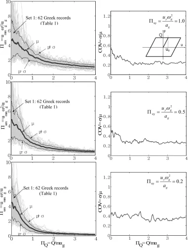
Figure 7 (left) plots the self-similar response spectra of the elastic-plastic system, for all the

selected ground motions of Table 1 and for different dimensionless yield displacements Πuy =

1.0 (top), 0.5 (middle) and 0.2 (bottom). Also, in Figure 7 (right) the corresponding coefficient

of variation (COV) is illustrated. Hence, the proposed approach can also be evaluated in terms

of reducing the scatter in the response. It is shown that the COV remains in most cases below

0.4, which is reasonably low (in an earthquake engineering context). As a general trend the

COVs increase as the dimensionless yield displacements decrease, but in all cases the COVs

range (Figure 7 right) between 0.2 and 0.4,.

Figure 8 presents the same plots as Figure 7 for the second set of records, which is identical

with the one used by Kappos & Kyriakakis [9]. Note that when compared with the COV

estimated in the study of Kappos & Kyriakakis the proposed approach yields equal or even

smaller scatter than the optimal of Kappos & Kyriakakis. It is recalled here that the study of

Kappos & Kyriakakis concerned the same mechanical configuration and excitations, but it

differed in the concept of describing the behaviour, which was based on ductility in lieu of the

dimensionless Π-terms proposed herein. This observation underlines the ability of the

0 1 2 3 4 0 0.2 0.4 0.6 0.8 1 1.2

0 1 2 3 4

0 2 4 6 8 10 μ μ+σ μ-σ

0 1 2 3 4

0 0.2 0.4 0.6 0.8 1 1.2

0 1 2 3 4

0 2 4 6 8 10 μ μ+σ μ-σ

0 1 2 3 4

0 0.2 0.4 0.6 0.8 1 1.2

0 1 2 3 4

0 2 4 6 8 10 μ μ+σ μ-σ 2 uy 1.0 y g g u a     Π um = u ma x ω g

2/α

g

Set 1: 62 Greek records (Table 1) CO V = σ / μ u F Q uy 2 uy 0.2 y g g u a     Π um = u m ax ω g

2/α

g

Π_Q= Q/mα_g

CO V = σ / μ

Π_Q= Q/mα_g

Set 1: 62 Greek records (Table 1) CO V = σ / μ 2 uy 0.5 y g g u a    

Set 1: 62 Greek records (Table 1) Π um = u m ax ω g

2/α

g

0 1 2 3 4 0 0.2 0.4 0.6 0.8 1 1.2

0 1 2 3 4

0 0.2 0.4 0.6 0.8 1 1.2

0 1 2 3 4

0 0.2 0.4 0.6 0.8 1 1.2

0 1 2 3 4

0 2 4 6 8 10 μ μ+σ μ-σ

0 1 2 3 4

0 2 4 6 8 10 μ μ+σ μ-σ

0 1 2 3 4

0 2 4 6 8 10 μ μ+σ μ-σ Π

Q= Q/mαg

Π

Q= Q/mαg

u F

Q

uy Set 2: 21 Greek records

(Table 1) 2 uy 0.2 y g g u a     2 uy 1.0 y g g u a     2 uy 0.5 y g g u a



Set 2: 21 Greek records (Table 1) Set 2: 21 Greek records

(Table 1) Π um = u ma x ω g

2/α

g Π um = u ma x ω g

2 /α

g Π um = u ma x ω g

2/α

g CO V = σ / μ C OV= σ / μ C OV= σ / μ

4.2 Pounding Oscillator subjected to base excitation of arbitrary shape

With reference to Figure 9 and following exactly the same procedure as for the elastic-plastic

system, the behaviour of the pounding oscillator can be described using the following

dimensionless Π-terms (for more details see [6]):

2 2

max

um ω δ ε ξ 0

0

( , , , ) g g, g , ,

N

g g

u

a a



 





 



 

        _ _

  (4)

where: ω0 =2π/T0, is the angular frequency and ξ0 the damping ratio of the oscillator, εΝ the

coefficient of restitution, δ the size of the gap, and the two parameters which describe the

excitation: the length scale, αg = PGA, and time scale, ωg =2π/Tm (Tm is the mean period, see

equation 1).

Again, the response spectra of the pounding oscillator (Figure 9 left) for a given

dimensionless gap, Πδ, become self-similar and when expressed in the proposed dimensionless

terms, collapse to a single master-curve. It is reminded that in the present study, no reference

has been made to typical pulses (unlike in Dimitrakopoulos et al. [6, 7]). The response under

ground motions with arbitrary shape, has been scaled directly to the excitation. Furthermore, the

proposed approach yields also considerably low scatter in the reponse, since the coefficient of

variation ranges between 0.2 and 0.4 (Figure 9 right).

5. CONCLUSIONS

The aim of the present study wais to build on the dimensional-response-analysis approach

introduced in previous works of the authors, and generalize the use of dimensional analysis for

describing the response of yielding and pounding structures in the case of excitations without

distinct pulses, by proposing the appropriate time and length scales of excitations with arbitrary

0 1 2 3 4 0

0.2 0.4 0.6 0.8 1 1.2

0 1 2 3 4

0 2 4 6 8 10

μ

μ+σ

μ-σ

Π um

= u

m

ax

ω g

2 /α

g

Π_ω= ω₀/ω_g

δ

εΝ ω0 ξ0

u

g

u

_

δ 1.0

g

g

a



  

0

0.5 0.05

N

 

 

Set 1: 62reek records (Table 1)

0 0 0

C

OV =

σ

/

μ

Π_ω= ω₀/ω_g

Figure 9. Left: Self-similar response spectra of the pounding oscillator for the selected excitations (Table 1). (μ): mean value, (σ): standard deviation. Right: Coefficient Of

Variation

The proposed scales were selected among the available in literature strong ground-motion

parameters, according to predefined criteria. As length scale, the peak ground acceleration

(PGA) was adopted, and as time scale the mean period (Tm) [19]. When the response was

described in dimensionless terms that hinge upon those parameters (PGA, Tm), remarkable order

emerged: response spectra for any excitation level collapsed to a single master curve

(self-similarity). Furthermore, it was shown, that this is true for two fundamental mechanical

configurations of earthquake engineering, the elastic-plastic system and the pounding oscillator.

The present analysis finally concluded that the proposed approach is also efficient in

reducing the scatter in the results and thus, it is a superior method of describing the non-linear

REFERENCES

1. Makris N, Black CJ. Dimensional Analysis of Rigid-Plastic and Elastoplastic Structures under Pulse-Type Excitations. Journal of Engineering Mechanics (ASCE) 2004; 130 (9): 1006-1018

2. Makris N, Black CJ. Dimensional Analysis of Bilinear Oscillators under Pulse-Type Excitations. Journal of Engineering Mechanics (ASCE) 2004; 130 (9): 1019-1031

3. Barenblatt GI. Scaling, Self-Similarity, and Intermediate Asymptotics. Cambridge Cambridge University Press U.K., 1996

4. Sedov LI. Similarity and Dimensional Methods of Mechanics. New York: Academic Press, 1959

5. Makris N, Psychogios C. Dimensional Response Analysis of Yielding Structures with 1rst-Mode Dominated Response. Earthquake Engineering and Structural Dynamics 2006; 35: 1203-1224

6. Dimitrakopoulos EG, Makris N, Kappos AJ, Dimensional Analysis of Pounding Oscillators. 6th GRACM International Congress on Computational Mechanics, Thessaloniki 2008, 19-21 June

7. Dimitrakopoulos EG, Makris N, Kappos AJ. Dimensional Analysis of the Earthquake Induced Pounding between adjacent Oscillators. Earthquake Engineering & Structural Dynamics (in press published on-line) 2008;

8. Mavroeidis GP, Papageorgiou AS. A mathematical representation of near-fault ground motions. Bulletin of the Seismological Society of America 2003; 93 (3): 1099-1131

9. Kappos AJ, Kyriakakis P. A re-evaluation of scaling techniques for natural records. Soil Dynamics and Earthquake Engineering 2000; 20: 111-123

10. Alavi B, Krawinkler H. Effects of near-source ground motions on frame-structures The John A. Blume Earthquake Engineering Center, Stanford University, 2001

11. Makris N, Chang S. Effect of viscous, visco-plastic and friction damping on the response of seismic isolated structures. Earthquake Engineering Structural Dynamics 2000; 29: 85-107

12. Mavroeidis GP, Dong G, Papageorgiou AS. Near-fault ground motions, and the response of elastic and inelastic single-degree-of-freedom (SDOF) systems. Earthquake Engineering Structural Dynamics 2004; 33: 1023-1049

13. Bray JD, Rodriguez-Marek A. Characterization of forward-directivity ground motions in the near-fault region. Soil Dynamics and Earthquake Engineering 2004; 24: 815-828

14. Aldea A, Lungu D, Arion A, GIS mapping of seismic microzonation and Site effects in Bucharest Based on Existing seismic and Geophysical Evidence. Proceedings of the International Conference “Earthquake Loss Estimation and Risk Reduction” Bucharest, Ro.,. 2004, Oct. 24-26, 2002, 237-250

15. Hancock J, Bommer JJ. A State-of-Knowledge Review of the Influence of Strong-Motion Duration on Structural Damage. Earthquake Spectra 2006; 22 (3): 827-845

16. Hancock J, Bommer JJ. Using spectral matched records to explore the influence of strong-motion duration on inelastic structural response. Soil Dynamics and Earthquake Engineering 2007; 27: 291-299

18. Mylonakis G, Voyagaki E. Yielding oscillator subjected to simple pulse waveforms: numerical analysis & closed-form solutions. Earthquake Engineering Structural Dynamics 2006; 35: 1949–1974

19. Rathje EM, Abrahamson NA, Bray JD. Simplified Frequency Content Estimates of Earthquake Ground Motions. Journal of Geotechnical and Geoenviromental Engineering 1998; 124 (2): 150-159

20. Mylonakis G, Reinhorn AM. Yielding oscillator under Triangular Ground Acceleration Pulse. Journal of Earthquake Engineering 2001; 5 (2): 225-251

21. Housner GW. Intensity of Ground Motion During Strong Earthquakes Second Technical Report, Project Designation NR-081-095 CALTECH, Earthquake Research Laboratory, 1952

22. Kappos AJ. Analytical Prediction of the Collapse Earthquake for R/C Buildings: Suggested Methodology. Earthquake Engineering Structural Dynamics 1991; 20 (2): 167-176 23. Dimova S, Elenas A. Seismic intensity parameters for fragility analysis of structures with energy dissipating devices. Structural Safety 2002; 24: 1-28

24. Fajfar, P., Vidic, T., and Fischinger (1990) M. A measure of earthquake motion capacity to damage medium-period structures. Soil Dynamics and Earthquake Engineering, 9(5):236-242

25. Riddell R. On Ground Motion Intensity Indices. Earthquake Spectra 2007; 23 (1): 147-173

26. Makris N, Black CJ. Evaluation of Peak Ground Velocity as a ‘‘Good’’ Intensity Measure for Near-Source Ground Motions. Journal of Engineering Mechanics (ASCE) 2004; 130 (9): 1032-1044

27. Cabanas L, Benito B, Herraiz M. An Approach to the Measurement of the Potential Structural Damage of Earthquake Ground Motions. Earthquake Engineering Structural Dynamics 1997; 26: 79-92

28. Cosenza E, Manfredi G. Damage indices and damage measures. Prog. Struct. Engng Mater. 2000; 2: 50-59

29. Manfredi G, Polese M, Cosenza E. Cumulative demand of the earthquake ground motions in the near source. Earthquake Engineering Structural Dynamics 2003; 32: 1853-1865 30. Karakostas CZ, Athanassiadou CJ, Kappos AJ, Lekidis VA. Site-dependent design spectra and strength modification factors, based on records from Greece. Soil Dynamics and Earthquake Engineering 2007; 27: 1012–1027

abbreviated running title :

Dimensional Response Analysis for Records Without