Wind Farm Capital Cost Regression Model for
Accurate Life Cycle Cost Estimation
David McMillan Institute for Energy & Environment
University of Strathclyde Glasgow, UK [email protected]
Graham W. Ault Institute for Energy & Environment
University of Strathclyde Glasgow, UK
Abstract— Various studies over the last decade have attempted to forecast capital cost of wind power. The main assumption underpinning these models is that cost reductions will accrue indefinitely from technological learning over time. In this paper a regression model is proposed for wind farm capital cost which is based on commodities price and water depth rather than technological learning. With greater simplicity and certainty in the theoretical foundations of such a model, it is possible to gain realistic estimates of wind turbine capital cost. Such pragmatic and well-reasoned output is needed so that wind farm developers can understand their future risk exposure to price fluctuations in capital cost of plant.
Keywords- Wind Turbine; Capital cost; Regression Model; wind farm; CAPEX. (key words)
I. INTRODUCTION
This paper proposes that the key driver for wind farm capital expenditure (CAPEX) has not been captured in existing models. Several authors propose application of technological learning models, which we will demonstrate as being inappropriate for the current level of technical development of wind, particularly offshore wind. Instead we propose a model based on coupling capital cost with metals commodities indexation and water depth. This model makes intuitive sense due to the well known influence of water depth on cost, and the amount of metal utilised in wind turbine construction. This pertinent to offshore wind due to high metallic content of foundations and inter-array cabling. Furthermore, the simplicity of this model means it can be applied transparently to cost data in the future.
II. PREVIOUS WORK
Several authors have proposed use of a technological learning model to capture wind farm or wind turbine capital costs. The papers by Junginger et al. [1, 2] are cases in point. The authors first reviewed the work of several other authors in fitting theoretical experience curves for prediction of wind turbine cost. They took UK data from 1991 – 2001 and used it to fit an experience curve, resulting in a progress ratio of 81%. This means that with each doubling of worldwide capacity, the per-unit cost should reduce by 19%. The authors used their model to extrapolate results out to a time
horizon of 2020. Their UK data showed a turnkey installation price of approximately €1200/MW in 2001 at which point the global installed capacity of wind was approximately 20GW. By 2008 global capacity was around 120GW [3] implying that prices should have reduced significantly (since the capacity has been doubled twice since 2001), however current onshore projects are typically running at more than the €1200/MW figure used in 2001. According to the learning rate model, the cost should have dropped to around (0.812x1200) €790/MW. In the UK a recent low end estimate of capital cost is €1500/MW [4]. One can conclude that the global experience curve does not apply to this phase of wind turbine development, since the actual cost and the model-generated cost trend in opposite directions. This seems like a classic case of unjustified extrapolation on the part of authors utilizing such methodologies. These limitations are discussed by Greenacre et al. [5] however there is little transparency in their proposed alternative approach.
A. Data
Bilgili et al. [6] show capital cost data for a set of offshore wind farms installed from 2001 – 2007. Table 1 is produced by taking their data from this period and adding new projects for the period 2008 – 2011. Table 1 also contains water depth data. From overall CAPEX it is possible to deduce turbine and foundation cost by assuming this to be 52% of the overall project capital cost [7]. Table 1 shows generally increasing capital cost, directly at odds with models assuming technological learning is the prime mover of capital cost. Therefore the technological learning model should be replaced with an adequate model.
The main starting assumption adopted in this paper is that commodities pricing (particularly metal) and water depth, are instead the main drivers of wind turbine capital cost. The reason for these assumptions is that:
• Water depth is a good proxy for project complexity
TABLE I. CAPITAL COST FOR OFFSHORE
Project area commissioned Middelgrunden DK
Horns Rev DK Samsø DK North Hoyle UK Nysted DK Scroby Sabds UK Kentish Flats UK Barrow UK Egmond aan See NL Burbo Bank UK Lillgrunden S Lynn & Inner Downsig UK Alpha Ventus DL Horns Rev II DK Rhyl Flats UK Thanet UK Robin Rigg UK Gunfleet Sands UK Nysted II DK Baltic 1 DL Walney 1 (not inc. grid conn.) UK
Data for metals commodity pricing was obtained for the period 1999-2011 [35]. The data takes the form of a commodity metals price index (CMPI) produced by the International Monetary Fund, which is broadly representative of iron, steel and copper as used in wind turbine manufacture. Figure 1 is a plot of the index for the period 1999-2011. The index has roughly trebled in value since 2001. Furthermore, it can be seen that the index ha recovered to pre-2008 financial crisis levels as of end 201
Figure 1. Metals price index [18]. *2011 figure based on Jan
FFSHORE WIND PROJECTS.BILGILI ET AL.[6] AND ADDITIONAL SOURCES INDICATED
commissioned wind farm CAPEX €/MW water depth m mean water depth m 2001 1.2 3-8 [9] 5.5
2002 1.7 2-9 [10] 5.5 2003 1.3 12-18 [11] 15 2003 2 5-12 [12] 8.5 2003 1.5 6-9 [13] 7.5 2004 2 2-10 [12] 6 2005 1.8 5 [12] 5 2006 1.59 [14] 15-20 [14] 17.5 2006 1.85 [15] 18 [16] 18 2007 2 2-8 [17] 5 2007 1.8 4-13 [18] 8.5 2008 1.76 [19] 6.3-11.2 [20] 8.75 2008 3.00 [21] 30-40 [21] 35 2009 2.14 [22] 9-17 [23] 13 2009 2.40 [24] 6.5-12.5 [25] 9.5 2010 2.96 [26] 20-25 [26] 22.5 2010 2.78 [27] 0.5-17 [28] 8.75 2010 2.77 [29] 8 [30] 8 2010 1.93 [31] 6-12 [32] 9 2010 4.14 [33] 16-19 [33] 17.5 2011 3.10 [34] 19-28 [34] 23.5
Data for metals commodity pricing was obtained for the takes the form of a commodity metals price index (CMPI) produced by the International Monetary Fund, which is broadly representative of iron, steel and copper as used in wind is a plot of the index for the he index has roughly trebled in value since 2001. Furthermore, it can be seen that the index had 2008 financial crisis levels as of end 2010.
]. *2011 figure based on Jan-Oct 2011
III. REGRESSION A
We follow a straightforward least squares linear regression as explained in Draper and Smith [36
Wind farm CAPEX (€/MW) = y Water Depth (m) =
CMPI = x2
It is assumed the relationship can be explained by the linear dependency:
y=b0+ b1x1
b0 and b1 are estimated using least squares
After the water depth (x1) regression is completed, the CM
(x2) is regressed on the residuals (
outputs are then added to yield a combined model.
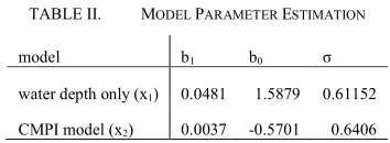
TABLE II. MODEL PARAMETER
model b1
water depth only (x1) 0.0481
CMPI model (x2) 0.0037
ES INDICATED. mean water depth m
ANALYSIS
follow a straightforward least squares linear ained in Draper and Smith [36], where:
€/MW) = y ) = x1 2
It is assumed the relationship can be explained by the
1 + ε (1)
are estimated using least squares (see Table II). regression is completed, the CMPI is regressed on the residuals (ε) of (1). The model outputs are then added to yield a combined model.
ARAMETER ESTIMATION
b0 σ
[image:2.612.348.525.594.659.2]IV. RESULTS
The model performance is firstly tested by plotting against the cost data in Table 1.
A. Model Testing
Figure 2 shows the first stage of modelling,
model regressed on water depth only. It can be seen that even a crude model based on water depth roughly
increasing cost seen in the data. This is in line with observations of similar recent studies [37].
robustness of this conclusion, Baltic 1 was removed from the data set and the model was re-fitted. The regression line for both cases is presented in Figure 3. The effect of removing Baltic 1 is to reduce the gradient of the regression line from 0.0481 to 0.0400. While this does weaken the correlation between CAPEX and water depth, removal of the data point cannot be justified until more information is available regarding any unique aspect of Baltic 1 which increased the project CAPEX. Therefore the data point is retained for subsequent analysis.
Figure 2. Regression model: water depth only (x
Figure 3. Regression line: water depth only (x1), excluding Baltic 1
firstly tested by plotting
Figure 2 shows the first stage of modelling, with the regressed on water depth only. It can be seen that even roughly captures the This is in line with ]. To test the robustness of this conclusion, Baltic 1 was removed from the The regression line for 3. The effect of removing Baltic 1 is to reduce the gradient of the regression line from While this does weaken the correlation between CAPEX and water depth, removal of the data point ormation is available regarding any unique aspect of Baltic 1 which increased the project CAPEX. Therefore the data point is retained for
Figure 2. Regression model: water depth only (x1)
), excluding Baltic 1
In the next stage, the CMPI data are used to fit a model to the residuals of the first model. Since the CMPI is an averaged value over a time scale of 1 year, the residuals have to be re-ordered according to the year of proje commissioning (see Table 1). The results of this regression model are shown in Figure 4, and the regression line in Figure 5. As can be seen in Table II, the influence of CMPI is an order of magnitude less than water depth. Nevertheless, the CMPI regression is included in
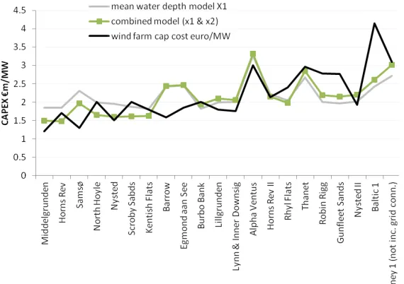
observe its effect on estimating the CAPEX. Figure 6 illustrates the performance of
(water depth only, and combined CMPI + water depth). Model output is plotted alongside
performance is evaluated via measuring the error of the two models.
The water depth model root mean squared error (RMSe) = 0.612 whereas the combined model RMSe
results obtained by the authors of [37
metals are statistically significant in overall project cost, but less so compared with the influence of
reinforces this conclusion.
Figure 4. Regression model:
Figure 5. Regression model: CMPI (
In the next stage, the CMPI data are used to fit a model to the residuals of the first model. Since the CMPI is an averaged value over a time scale of 1 year, the residuals have ordered according to the year of project le 1). The results of this regression , and the regression line in As can be seen in Table II, the influence of CMPI is an order of magnitude less than water depth. Nevertheless, sion is included in the model in order to observe its effect on estimating the CAPEX.
illustrates the performance of the 2 models (water depth only, and combined CMPI + water depth). Model output is plotted alongside the original data. Model easuring the error of the two
he water depth model root mean squared error (RMSe) combined model RMSe = 0.530. The s obtained by the authors of [37] suggest that cost of n overall project cost, but less so compared with the influence of water depth. Figure 6
Regression model: CMPI ( x2)
Figure 6
B. Forecasting
The model can be used in predictive mode to estimate future costs. For near shore shallow water projects of water depth = 20m, we can evaluate the scenario of a collapse in commodity prices, using 2008 CMPI index levels. Using values from Table II, firstly the CMPI contribution is calculated:
y=b0+ b1x2 + ε = -0.5701 + 0.0037 * 169.01 +
= 0.053845757 + ε
This is added to the water depth model, resolved at 20m depth:
y=b0+ b1x1 + ε = 1.5879 + 0.0481 * 20 + (0.053845757 +
= €2.60m/MW
Alternatively we can evaluate the project at the same water depth at current commodity cost levels:
y=b0+ b1x1 + ε = 1.5879 + 0.0481 * 20 + (0.305276716
= €2.85m/MW
This is equivalent to a CAPEX rise of nearly 10%.
Figure 6. Combined regression model (x1+ x2)
The model can be used in predictive mode to estimate future costs. For near shore shallow water projects of water depth = 20m, we can evaluate the scenario of a collapse in commodity prices, using 2008 CMPI index levels. Using s from Table II, firstly the CMPI contribution is
0.5701 + 0.0037 * 169.01 + ε
This is added to the water depth model, resolved at 20m
+ 0.0481 * 20 + (0.053845757 + ε)
Alternatively we can evaluate the project at the same water
0.305276716 + ε)
This is equivalent to a CAPEX rise of nearly 10%.
V. CONCLUSIONS
The research area of modelling and predicting wind capital cost has been dominated by technological learning models. These models do not explain the
trends seen in practice, which is a major flaw with such models. The parsimonious model prese
highly intuitive approach which can be tested and used easily. The result is greater confidence in the model.
Clearly water depth and materials are not the only driver in offshore wind farm capital cost. The other oft
are demand and supply bottlenecks. Manufacturing capacity data are not available in the public domain. However building annual demand into the model may result in a better fit.
Currency exchange rates are another possible source CAPEX coupling. Furthermore, nonlinear regression methods may be more appropriate for future estimates of capital cost. These issues will be explored in a future paper.
REFERENCES
[1] M. Junginger, A. Faaij, W. Turkenburg, Global experience curves for wind farms, Energy Policy. 33, 2 (2005) 133
[2] M. Junginger, A. Faaij, W. Turkenburg, Cost Reduction Prospects f Offshore Wind Farms, Wind Engineering. 28, 1 (2004) 97
[3] GWEC. Installed Capacity Data Summary, http://www.ewea.org/fileadmin/ewea_documents/documents/statistics/gwe c/GWEC_-_Table_and_Statistics_2009.pdf; 2009 (accessed 10.08.11). [4] Mott McDonald. UK Electricity Generation Costs Update, http://www.decc.gov.uk/assets/decc/statistics/projections/71
generation-costs-update-.pdf; June 2010 (accessed 10.08.11).
[5] P. Greenacre, R. Gross, P. Heptonstall, Great Expectations: The cost of offshore wind in UK waters – understanding the past and projecting the future. September 2010.
ONCLUSIONS
The research area of modelling and predicting wind farm capital cost has been dominated by technological learning models. These models do not explain the recent upwards cost , which is a major flaw with such . The parsimonious model presented here provides a can be tested and used . The result is greater confidence in the model.
Clearly water depth and materials are not the only drivers cost. The other oft-cited factors y bottlenecks. Manufacturing capacity data are not available in the public domain. However building annual demand into the model may result in a better
change rates are another possible source of Furthermore, nonlinear regression methods may be more appropriate for future estimates of ost. These issues will be explored in a future paper.
EFERENCES
[1] M. Junginger, A. Faaij, W. Turkenburg, Global experience curves for wind farms, Energy Policy. 33, 2 (2005) 133-150.
[2] M. Junginger, A. Faaij, W. Turkenburg, Cost Reduction Prospects for Offshore Wind Farms, Wind Engineering. 28, 1 (2004) 97-118.
[3] GWEC. Installed Capacity Data Summary, http://www.ewea.org/fileadmin/ewea_documents/documents/statistics/gwe
_Table_and_Statistics_2009.pdf; 2009 (accessed 10.08.11). ld. UK Electricity Generation Costs Update,
http://www.decc.gov.uk/assets/decc/statistics/projections/71-uk-electricity-.pdf; June 2010 (accessed 10.08.11).
[6] M. Bilgili, A. Yasar, E. Simsek, Offshore wind power development in Europe and its comparison with onshore counterpart, Renewable and Sustainable Energy Reviews. 15 (2011) 905–915.
[7] ODE. Study of the Costs of Offshore Wind Generation, http://webarchive.nationalarchives.gov.uk/+/http://www.berr.gov.uk/files/fi le38125.pdf; 2007 (accessed 10.08.11).
[8] E. Martinez, F. Sanz, S. Pellegrini, E. Jimenez, J. Blanco, Life cycle assessment of a multi-megawatt wind turbine, Renewable Energy 34 (2009) 667–673.
[9]Middelgrunden project data. Accessed 1st
Dec. 2011. http://www.middelgrunden.dk/middelgrunden/sites/default/files/public/file/ Artikel%20Copenhagen%20Offshore%207%20Middelgrund.pdf [10]Horns Rev project data. Accessed 1st Dec. 2011. http://www.hornsrev.dk/Miljoeforhold/miljoerapporter/Baggrundsrapport_ 8.pdf
[11] Samso project data. Accessed 1st Dec. 2011.
http://www.energy.siemens.com/hq/pool/hq/power-generation/wind-power/Offshore%20wind%20power%20projects.pdf
[12] N. Hoyle, Scroby Sands & Kentish Flats project data. Accessed 1st
Dec. 2011. http://www.wind-energy-the-facts.org/en/part-3-economics-of-wind-power/chapter-2-offshore-developments/
[13] Nysted project data. Accessed 1st
Dec. 2011. http://www.energy.siemens.com/hq/pool/hq/power-generation/wind-power/Offshore%20wind%20power%20projects.pdf
[14] Barrow project data. Accessed 1st Dec. 2011.
http://www.lorc.dk/Knowledge/Offshore-renewables-map/Offshore-site-datasheet/Barrow-Offshore-Wind-Farm/000024?free=barrow
[15]Power-Technology Industry Projects. Egmond aan Zee, http://www.power-technology.com/projects/egmond/; (accessed 10.08.11). [16] Egmond aan Zee project data. Accessed 1st
Dec. 2011. http://www.lorc.dk/Knowledge/Offshore-renewables-map/Offshore-site-datasheet/Egmond-aan-Zee-Offshore-Wind-Farm/000023
[17] Burbo Bank project data. Accessed 1st
Dec. 2011. http://www.lorc.dk/Knowledge/Offshore-renewables-map/Offshore-site-datasheet/Burbo-Bank-Offshore-Wind-Farm/000029
[18] Lillgrunden project data. Accessed 1st
Dec. 2011. http://www.energy.siemens.com/hq/pool/hq/power-generation/wind-power/Offshore%20wind%20power%20projects.pdf
[19] Power-Technology Industry Projects. Lynn and Inner Dowsing, http://www.power-technology.com/projects/lynnandinnerdowsing/; (accessed 10.08.11).
[20] http://www.lorc.dk/Knowledge/Offshore-renewables-map/Offshore-site-datasheet/Lynn-Offshore-Wind-Farm/000033
[21]Waldermann A. A Green Revolution off Germany's Coast. Spiegel. http://www.spiegel.de/international/germany/0,1518,567622,00.html; July 2008 (accessed 10.08.11).
[22] Nordic Investment Bank. Where the wind blows: Horns Rev II, http://www.nib.int/news_publications/cases_and_feature_stories/dong_ener gy_2008; October 2008 (accessed 10.08.11).
[23] http://www.lorc.dk/Knowledge/Offshore-renewables-map/Offshore-site-datasheet/Horns-Rev-2-Offshore-Wind-Farm/000036
[24] May J, RWE. North Hoyle and Rhyl Flats Offshore Wind Farms: Review of good practice in monitoring, construction and operation, http://www.snh.org.uk/pdfs/sgp/A303575.pdf; July 2009 (accessed 10.08.11).
[25]http://www.lorc.dk/Knowledge/Offshore-renewables-map/Offshore-site-datasheet/Rhyl-Flats-Offshore-Wind-Farm/000044
[26]Power-Technology Industry Projects. Thanet Array, http://www.power-technology.com/projects/thanetwindfarm/; (accessed 10.08.11).
[27]Marine Scotland. Robin Rigg Offshore Case Study, http://www.scotland.gov.uk/Resource/Doc/295194/0105826.pdf; 2010 (accessed 10.08.11).
[28] Robin Rigg project data. Accessed 1st
Dec. 2011. http://www.vindselskab.dk/media(2857,1030)/Kaj_Lindvig.pdf
[29]BBC. Gunfleet Sands Project Update, http://news.bbc.co.uk/1/hi/england/essex/8026694.stm; April 2009 (accessed 10.08.11).
[30]http://www.energy.siemens.com/hq/pool/hq/power-generation/wind-power/Offshore%20wind%20power%20projects.pdf
[31]4C Offshore. Rödsand 2, http://www.4coffshore.com/windfarms/rodsand-ii-denmark-dk11.html; (accessed 10.08.11).
[32] Rodsand 2 project data. Accessed 1st
Dec. 2011. http://www.lorc.dk/Knowledge/Offshore-renewables-map/Offshore-site-datasheet/Roedsand-2-Offshore-Wind-Farm/000046
[33] Baltic-1 project data. Accessed 1st Dec. 2011.
http://www.lorc.dk/Knowledge/Offshore-renewables-map/Offshore-site-datasheet/Baltic-1-Offshore-Wind-Farm/52
[34] Walney project data. Accessed 1st
Dec. 2011. http://www.4coffshore.com/windfarms/walney-phase-1-united-kingdom-uk31.html
[35]Indexmundi. Commodity Metals Price Index by Month, http://www.indexmundi.com/commodities/?commodity=metals-price-index&months=120; 2011 (accessed 10.08.11).
[36] N.R. Draper, H. Smith, Applied Regression Analysis, third ed., Wiley Probability and Statistics, 1998.