Taylor, Alan and Higham, Desmond J., EPSRC Grants (Funder) (2009)
CONTEST : a Controllable Test Matrix Toolbox for MATLAB. ACM
Transactions on Mathematical Software, 35 (4). 26:1-26:17. ISSN
0098-3500 , http://dx.doi.org/10.1145/1462173.1462175
This version is available at https://strathprints.strath.ac.uk/15066/
Strathprints is designed to allow users to access the research output of the University of Strathclyde. Unless otherwise explicitly stated on the manuscript, Copyright © and Moral Rights for the papers on this site are retained by the individual authors and/or other copyright owners. Please check the manuscript for details of any other licences that may have been applied. You may not engage in further distribution of the material for any profitmaking activities or any commercial gain. You may freely distribute both the url (https://strathprints.strath.ac.uk/) and the content of this paper for research or private study, educational, or not-for-profit purposes without prior permission or charge.
Any correspondence concerning this service should be sent to the Strathprints administrator:
The Strathprints institutional repository (https://strathprints.strath.ac.uk) is a digital archive of University of Strathclyde research outputs. It has been developed to disseminate open access research outputs, expose data about those outputs, and enable the
for MATLAB
ALAN TAYLOR and DESMOND J. HIGHAM University of Strathclyde
1. MOTIVATION
Networks describing connectivity structures arise across a vast range of application areas. Examples where it has proved useful to record data include interactions be-tween genes [Kauffman 1969], proteins [de Silva and Stumpf 2005], cortical regions [Kamper et al. 2002; Sporns and Zwi 2004], internet nodes [Faloutsos et al. 1999], web pages [Broder et al. 2000; Page et al. 1998], countries [Fagiolo 2007], co-authors [Newman 2004], telephones [Abello et al. 1998], assets on the stock market [Bogin-ski et al. 2003] and members of various populations [Conyon and Muldoon 2006; Kiss et al. 2006; Onody and de Castro 2004; Porter et al. 2005; Williams et al. 2002].
Typical data mining and visualisation tasks reduce to linear system or eigenvalue computations with the large, sparse adjacency matrices that define the interactions. Several random graph models, that is, formulas for probabilistically inserting con-nections, have been derived that attempt to capture the key topological properties of real-life networks. Important goals for such work are to understand how a network has reached its current state and to predict how it will evolve. From a numerical analysis perspective, these random graph models are an extremely useful source of realistic, controllable test matrices for linear algebra software. This provides the motivation for the MATLAB toolbox CONTEST (CONtrollable TEST matrices), which implements nine popular random network models, along with various util-ity functions for post-processing the networks. CONTEST is available from the website
http://www.maths.strath.ac.uk/research/groups/numerical_analysis/contest
The codes were developed and tested under MATLAB Version 7.4.0.287 (R2007a). As supplementary material at the website, we record performance results for
MAT-LAB’s built-in iterative linear system solverspcg,qmr,symmlq,lsqr,minres,cgs,
gmres,bicgandbicgstabusing test matrices from the toolbox.
Department of Mathematics, University of Strathclyde, Glasgow, G1 1XH, UK. DJH was supported by Engineering and Physical Sciences Research Council grants GR/S62383/01 and EP/E049370/1.
Permission to make digital/hard copy of all or part of this material without fee for personal or classroom use provided that the copies are not made or distributed for profit or commercial advantage, the ACM copyright/server notice, the title of the publication, and its date appear, and notice is given that copying is by permission of the ACM, Inc. To copy otherwise, to republish, to post on servers, or to redistribute to lists requires prior specific permission and/or a fee.
c
·
This article is arranged as follows. Section 2 gives a very brief overview of the historical development of random network models. In section 3 we describe each of the nine models and the corresponding MATLAB code. Section 4 introduces the utility functions for altering existing networks, setting up coefficient matrices arising in common tasks and checking some basic topological properties. In section 5 we give a very brief illustration of the toolbox in use, and we summarize the aims of this work in section 6.
Our notation is as follows. We letndenote the number of nodes in a network,
withaij=aji= 1 if nodesiandjare connected andaij=aji= 0 otherwise. So the
adjacency matrixA∈Rn×nis symmetric. We always havea
ii = 0; so nodes cannot
be self-connected. Thedegreeof nodeiis found by counting its neighbours, degi:=
Pn
j=1aij. For degi >1 the curvature or clustering coefficient of node i is found
by counting how many pairs of these neighbours are themselves connected, and
dividing this number by the maximum possible number of connections, degi(degi−
1)/2. A definition in terms of MATLAB comands is given in section 4.7.1.
A call to one of the random network functions in the toolbox will generate an
A∈Rn×n as an independent instance drawn from a random network model. The
randomness is driven entirely by MATLAB’s built in pseudo-random number
gen-erators, rand and randn, and our codes do not alter their states. So the user
can get back the same matrix by re-setting the states of these two random num-ber generators. For consistency, we always generate adjacency matrices with the
sparse attribute, even though for some parameter values a full matrix may arise
(for example, with the extreme choice ofp= 1 in the Gilbert model of section 3.1).
Although we produce only symmetric adjacency matrices, it is straightforward to create unsymmetric versions, corresponding to directed networks, by combining the upper and lower triangles from two independent samples from the same model. For
example, callingA = erdrey(n,m)andB = erdrey(n,m), whereerdreydescribed
in section 3.1.1 implements the Erd˝os–R´enyi model, we could set C = triu(A) +
tril(B).
2. BACKGROUND
It has been repeatedly observed that real connectivity networks are neither com-pletely regular lattices nor classical random graphs. Following the landmark paper of Watts and Strogatz [Watts and Strogatz 1998], there has been a resurgence of interest in the idea of designing probabilistic models that capture important
topo-logical properties of real networks. Watts and Strogatz coined the phrase small
world network to describe a regime where small pathlengths coexist with large
clustering coefficients (nodes tend to live in cliquey, well-connected subgraphs and yet the network can be globally traversed with relatively few links). They also showed that this pair of properties arise when an appropriate amount of disorder is added to a regular lattice.
Another key property that is claimed to be common in real networks is ascale-free
degree distribution,
Number of nodes of degreek
n ∝k
−γ, (1)
model of Barab´asi and Albert [Barab´asi and Albert 1999] attempts to describe the way a network might grow when new nodes are added and new connections formed, and it produces scale-free degree distributions. More recently, however, the prevalence of the scale-free property has been questioned, at least in the context of biological networks [Khanin and Wit 2006; Prˇzulj et al. 2004; Stumpf et al. 2005].
In addition to small worlds and scale-freeness, a third dominant concept is that
ofmotifs [Alon 2006; Milo et al. 2004]. A motif is a subgraph that is significantly
overrepresented (relative to the occurrence of that subgraph in a “randomized” version of the network). These motifs may be regarded as the basic building blocks of the networks, and hence understanding their roles gives valuable insights into how the overall network operates [Mangan and Alon 2003; Mangan et al. 2003].
The closely related idea ofgraphlet frequency was introduced in [Prˇzulj et al. 2004]
as a means to compare networks and further developed in [Prˇzulj et al. 2006]. Two networks are “close” if they are made up of building blocks in the same relative proportions. This gives a powerful and comprehensive means to check whether a probabilistic model is capturing topological properties of real networks and to decide which models are most appropriate. Using these ideas, the software tool GraphCrunch for network comparison was developed in [Milenkovic et al. 2008].
Overall, a recent and rapid expansion in theoretical and empirical research ac-tivity has produced several models for computing networks in a controlled manner that are “close” to real life networks in a well-defined sense. It is our tenet that these computable networks are therefore excellent candidates for test matrices.
Although well established sparse matrix test sets exist, [Boisvert et al. 1997; Davis 2007; Duff et al. 1989], they have been built around fixed instances arising in particular application areas. Randomness is typically incorporated very sim-plistically. For example, Matrix Market [Boisvert et al. 1997] with website URL
http://math.nist.gov/MatrixMarket/ makes available the random generators
DLATMR/ZLATMRfrom LAPACK [Anderson et al. 1999], which independently assign random samples from a given distribution across the entries of an array and then randomly reset elements to zero in order to achieve a given level of sparsity. In [Davis 2007], Davis argues that “random sparse matrices” are not appropriate for testing sparse matrix algorithms; however, those comments would appear to be aimed at different classes of matrices to those considered here. The models im-plemented in CONTEST use randomness to capture properties that are commonly observed in complex interaction networks.
The code in CONTEST was written to exploit vectorization and to use matrix-vector level operations where possible, but ultimately our priority was to allow sparse matrices of the largest possible dimension to be computed. A secondary aim was produce short, readable and maintainable programs. The importance of mem-ory allocation and usage when generating sparse matrices in MATLAB is discussed
in [Gilbert et al. 1992] and in NA Digest athttp://www.netlib.org/na-digest-html/07/v07n28.html#1.
·
0 50 100
0 20 40 60 80 100
nz = 462 erdrey(100)
0 50 100
0 20 40 60 80 100
nz = 474 gilbert(100)
0 50 100
0 20 40 60 80 100
nz = 408 smallw(100)
0 50 100
0 20 40 60 80 100
nz = 440 geo(100)
0 50 100
0 20 40 60 80 100
nz = 373 pref(100)
0 50 100
0 20 40 60 80 100
nz = 1740 renga(100)
0 50 100
0 20 40 60 80 100
nz = 588 kleinberg(100)
0 50 100
0 20 40 60 80 100
nz = 871 lockandkey(100)
0 50 100
0 20 40 60 80 100
[image:5.612.88.471.82.408.2]nz = 184 sticky(100)
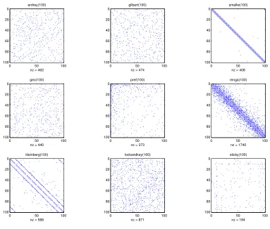
Fig. 1. Spy plots showing nonzero patterns for a 100×100 sample from each of the nine models.
3. MODELS
In this section, we give brief descriptions of the nine models implemented, and show how to use the corresponding MATLAB functions. In each case, the output
argument, A, is a sparse, symmetric, zero-diagonal matrix of dimensionn, with n
being the first of the input arguments. The remaining input arguments take default values if not specified in the function call. Default parameters have been chosen to
ensure thatAcorresponds to a connected (irreducible) graph with high probability,
with the exception ofstickyin section 3.7.1, which, by construction, may produce
many small disconnected subgraphs. In Figure 1 we show a spy plot for each of
the nine models usingn=100; this dimension was chosen to make the visualisation
3.1 Classical
Random graph theory began in earnest in the late 1950s, with the two classical
models in [Gilbert 1959] and [Erd¨os and R´enyi 1959]. These models are usually
referred to as G(n, p) andG(n, m), but to help distinguish between them we will
use the names Gilbert and Erd˝os–R´enyi.
In Gilbert’s model [Gilbert 1959] a fixed probability p is specified, and then
each pair of nodes is, independently, connected with probabilityp. In the Erd˝os–
R´enyi model [Erd¨os and R´enyi 1959] the number, m, of edges in the network is
specified. (Of course, mmust be no more than the maximum possible number of
edges,n(n−1)/2.) We then select uniformly at random from the set of all graphs
containingnnodes andmedges.
The properties of these classical random graphs have been well studied [Albert
and Barab´asi 2002; Bollob´as 1985], although in terms of currently adopted
mea-sures, such as pathlengths, clustering coefficients and graphlet frequencies, they cannot be regarded as accurate models of realistic networks [de Silva and Stumpf 2005; Prˇzulj et al. 2004; Watts and Strogatz 1998]. Our implementation for the Gilbert class is taken from [Batagelj and Brandes 2005, Algorithm 1].
3.1.1 Classical Codes: gilbert and erdrey. The function gilbert(n,p)
re-turns an instance from the Gilbert class. The optional second input argument
de-faults to log(n)/n, soA = gilbert(n)is equivalent toA = gilbert(n,log(n)/n).
Similarly,A = erdrey(n,m)produces an Erd˝os–R´enyi random graph, withm
de-faulting to the smallest integer bigger thannlog(n)/2.
3.2 Small World
Motivated by the “small world” concept of the experimental psychologist Stanley Milgram [Milgram 1967], Watts and Strogatz [Watts and Strogatz 1998] proposed a random graph model that can be regarded as interpolating between a regular, periodic lattice and a classical random graph. Although the original work used re-wiring, it is now more common to introduce randomness via the addition of short-cuts [Higham and Higham 2000; Newman et al. 2000]. Hence, in our Watts-Strogatz
model we begin with a k-nearest neighbour ring (nodes i and j are connected if
and only if |i−j| ≤k or |n− |i−j|| ≤ k). Then, each node is considered
inde-pendently in turn. With fixed probabilitypa node is given an extra link—a short
cut—connecting it to a node chosen uniformly at random across the network. (At the end of this process, self links and repeated links between nodes are removed.)
3.2.1 Small World Code: smallw. The function smallwreturns an instance of
the Watts-Strogatz model, with syntax according to A = smallw(n,k,p). The
optional input argumentsk and p default to 2 and 0.1, respectively. From a
lin-ear algebra perspective, the adjacency matrix has a symmetric, banded Toeplitz structure, with extra nonzeros added uniformly and symmetrically at random. We
note thatsmallwmakes use of the utility function shortthat is described in
·
3.3 Geometric
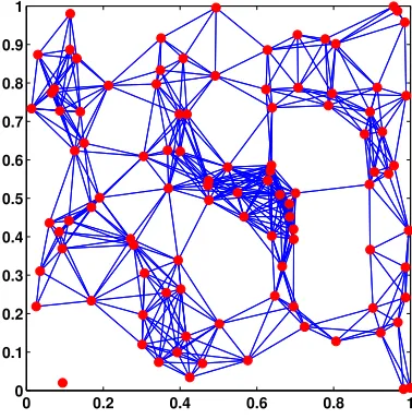
A two-dimensional, non-periodic, geometric random graph may be defined as
fol-lows. First, each of thennodes is placed at random in the unit square—more
pre-cisely, theith node is given coordinates (xi, yi), where{xi, yi}ni=1 are independent
and identically distributed with uniform (0,1) distribution. Next, for some specified radius, r, nodesi and j are connected if and only if (xi−xj)2+ (yi−yj)2 ≤r2.
In words, an edge denotes that two nodes were placed no more than Euclidean
distancerapart. Figure 2 illustrates the process withn= 100 and r= 0.2.
0 0.2 0.4 0.6 0.8 1
[image:7.612.208.397.186.378.2]0 0.1 0.2 0.3 0.4 0.5 0.6 0.7 0.8 0.9 1
Fig. 2. Construction of a geometric random graph. Here,n= 100 andr= 0.2.
We emphasize that the resulting graph is simply the usual list of nodes and edges. Information about the precise locations {xi, yi}ni=1 is not part of the final
mathematical object. Natural generalizations are possible.
Dimension:. the nodes can be randomly assigned to locations in the unit cube
inRm, for somem >2.
Periodicity:. distance can be measured in a wrap-around fashion, so that, for
example, in the unit square, (xi−xj)2+ (yi−yj)2is replaced by
(min (|xi−xj|,1− |xi−xj|))
2
+ (min (|yi−yj|,1− |yi−yj|))
2
.
Norm:. the Euclidean norm can be replaced by any other vector norm.
3.3.1 Geometric Code: geo. The call A = geo(n,r,m,per,pnorm)returns an instance of a geometric random graph. There are four optional input arguments:
—rspecifies the radius, defaulting top1.44/n, which is motivated by the
asypm-totic (n → ∞) level that guarantees connectivity in two dimensions [Penrose
2003].
—mspecifies the dimension, defaulting to 2,
—peris a logical variable specifying whether periodic distance is to be used,
de-faulting toper = 0; not periodic,
—pnormspecifies the Lp-norm to be used, defaulting to 2.
3.4 Preferential Attachment
Barab´asi and Albert [Barab´asi and Albert 1999] used the concept of preferential
attachment to develop random graphs with scale-free degree distributions. In this model, the network grows—new nodes are added and linked in to the existing
network—untilnnodes have been created. For some fixed integerd≥1, each new
node is givendlinks on arrival. These new connections are not chosen unformly;
the new node links to an existing node with a probability that is proportional to the current degree of that node. In this way, well-connected nodes tend to become even better connected (the rich get richer) as the network evolves. Our precise model is a translation into MATLAB of [Batagelj and Brandes 2005, Algorithm 5], which uses the specification in [Bollob´as et al. 2001].
3.4.1 Preferential Attachment Code: pref. The call A = pref(n,d) returns
an instance of a preferential attachment graph, using a single node as the initial
network. The degree parameterddefaults to 2.
3.5 Range Dependent
3.5.1 RENGA. Yeast two hybrid protein-protein interaction (PPI) networks
have proteins as nodes. Two nodes share an undirected edge if they have been experimentally observed to interact [Xenarios et al. 2002]. Motivated by the struc-ture of PPI networks, Grindrod [Grindrod 2002] proposed and analyzed a random graph model that, in a sense, generalizes Watts–Strogatz. In this model, the nodes have a natural linear ordering,i= 1,2, . . . , n. Independently over all pairs of nodes, we then insert a link between nodesiandjwith probabilityαλ|j−i|−1, whereα >0
and λ∈(0,1) are fixed parameters. The choiceα= 1 ensures that adjacently
or-dered nodes are always connected. The geometric factorλ|j−i|−1causes long-range
edges to be less common than short-range edges.
Further analysis and generalizations of this model, now refered to as RENGA, appear in [Grindrod et al. 2008; Higham 2003; 2005]. Closely related models have also been used in percolation theory [Grimmett 1999].
3.5.2 RENGA Code: renga. The callA = renga(n,lambda,alpha)returns an
instance of a RENGA, withlambdadefaulting to 0.9 andalphadefaulting to 1.
3.5.3 Kleinberg. Kleinberg [Kleinberg 2000] defined a variation of the
two-·
dimensional lattice: the n=m2 nodes can be thought of as being equally spaced
throughout a square, with each node having a location of the form (i, j)∈R2where
the integersiandj run from 1 tom. Every node is given short range connections
to its neighbours that are a lattice (Manhattan) distance of at mostpaway. Then
each node is given q further ‘long-range’ connections. For a given node, u, the
recipient,v, of each such long-range connection is chosen independently at random,
with probability proportional tor−α. Here,ris the lattice distance betweenuand
v andα≥0 is a fixed parameter.
3.5.4 Kleinberg Code: kleinberg. The callA = kleinberg(n,p,q,alpha)
gen-erates an instance of the Kleinberg model. If the input dimension,n, is not a perfect
square then the output matrix has dimension(round(sqrt(n)))^2. Default values
arep = 1,q = 1andalpha = 2.
3.6 Lock and Key
Using some basic biological insights, Thomas et al. [Thomas et al. 2003] proposed a class of random graphs that model PPI networks. This class of models was further analysed in [Morrison et al. 2006], where it was used to extract new biological information from real PPI data sets. The underlying modeling idea is that two proteins interact because they share physically matching parts, which, following
[Morrison et al. 2006], we refer to aslocks andkeys. There will be several different
types of key, which we can think of as labeled by colors (red, green, blue, etc.) and for each type of key there is a matching lock (red, green, blue, etc.). In the model, each protein has the same chance of possessing each color of lock and each color
of key. More precisely, for a given number of colors,m, we take each node in turn
and independently assign it each possible lock and key with some fixed probability
p. The graph is then generated according to the rule that two nodes share an edge
if and only if one possesses a key and the other possesses a lock of the same color. Self links are removed.
3.6.1 Lock and Key Code: lockandkey. The callA = lockandkey(n,m,p)
re-turns an instance of a lock and key graph where there are m different lock and
key colors and each type of lock and key is handed out independently with fixed
probabilityp. Default values arem = ceil(n*log(n))andp = 1/n.
3.7 Stickiness
The stickiness model was introduced in [Prˇzulj and Higham 2006] to model PPI networks. It was motivated as a simplified version of the lock and key framework in
which parameters could be fitted to real data. Here, a nonnegative vector db∈Rn
is given, representing the scaled degree distribution of some target network; more precisely, dbi = degi/
qPn
j=1degi, where degi is the degree of theith node in the
target. Then a new random network is produced by connecting nodesiandjwith
probabilitydbidbj. In this way theexpected degrees in the random model match the
target degrees. This model was found to be more accurate than previously proposed models at reproducing topological properties of PPI networks.
3.7.1 Stickiness Code: sticky. The call A = sticky(deg) generates an
one-dimensional arraydeg. To be consistent with our general philosophy that all
mod-els can be called with a single input argument,n, representing the dimension, we
allow an exception where sticky is called as A = sticky(n), with n a positive
integer. In this caseAwill be an instance of a stickiness graph of dimensionnwith
a scale-free expected degree distribution of the form (1) with γ = 2.5. It is also
possible to specify two input parameters, a callA = sticky(n,gamma)specifies the
value ofγto be used in (1).
4. UTILITY FUNCTIONS 4.1 Rewiring
The Watts-Strogatz model [Watts and Strogatz 1998] added randomness to a ring
network by rewiring some edges. For a general undirected network, we define a
rewiring process as follows, in terms of a fixed parameter p. Each entry in the
lower triangle of the original adjacency matrix is examined in turn. Ifaij 6= 0 then,
independently with probabilityp, we resetaij =aji= 0, choose a nodekuniformly
at random from all non-neighbours of nodei, and setaik=aki= 1.
4.1.1 Rewiring Code: rewire. The call R = rewire(A,p) takes an adjacency
matrix A and returns a rewired adjacency matrix R. The rewiring probability p
defaults top = log(n)/n.
4.2 Shortcuts
Rewiring has the theoretical drawback that it may cause a connected network to
become unconnected. Addingshortcutsis an alternative procedure that gives very
similar topological effects [Newman et al. 2000] but does not degrade connectivity.
In this case the parameterpis a fixed a probability that is used independently over
all nodes. For each node, with probabilitypwe add a new link from that node to
a node chosen uniformly at random across the whole network. Self links are then removed and repeated links treated as single links.
4.2.1 Shortcut Code: short. The callS = short(A,p)takes an adjacency
ma-trixA, adds shortcuts and returns the new adjacency matrixS. The shortcut
prob-abilitypdefaults tolog(n)/n.
4.3 Subsampling
Information is often missing from real life connectivity data sets [de Silva et al. 2006]. These omissions may be caused, for example, by errors in experimental observations (false negatives) or by an inherent restriction on the number or type of observations that can be made. In the case of yeast two hybrid PPI networks, it is widely accepted that the reported network is merely a noisy subset of the underlying “true” network, and we can think of the given network as being generated from a “subsampling” operation on the larger version [Titz et al. 2004]. Interestingly, it has been discovered that the subsampling operation may dramatically alter the topological properties of a network [de Silva et al. 2006; Han et al. 2005; Salath´e et al. 2005].
·
of those nodes and edges. The first algorithm does an unbiased, uniform node
removal involving a fixed parameterp. Each node is considered in turn, and with
independent probability 1−p we remove that node and all edges that involve it,
that is, we delete that row and column from the adjacency matrix. The second algorithm uses a bait and prey approach, along the lines of [Han et al. 2005], which models the generation of certain PPI data sets. Here, we use two fixed parameters,
baitandprey. A proportionbaitof the nodes are chosen as baits. Then, for each
bait, a proportion preyof its edges are recorded, along with the prey nodes that
are linked to the bait by those edges. The final subsampled network consists of the bait-prey edges and all the nodes that they involve.
4.3.1 Supsampling Codes: unisampleandbaitsample. The callU = unisample(A,p)
takes an adjacency matrixAand returns a subnetworkUformed from an unbiased,
uniform node removal. The probabilitypdefaults to0.5.
The bait and prey algorithm can be called as B = baitsample(A,bait,prey),
with defaultsbait = 0.5andprey = 0.5.
4.4 Laplacian Matrices
An undirected network can be characterised by its adjacency matrix, and basic linear algebra tells us that the eigenvectors and eigenvalues of this matrix carry relevant information. However, spectral graph theory [Chung 1997] has shown that it is generally more useful to look at the spectrum of the so-called Laplacian. There are two different matrices that take this name in the literature. We distinguish between them as follows.
—Thegraph Laplacian has the formD−A.
—Thenormalized graph Laplacian has the formDb−1
2(D−A)Db−12.
Here D= diag(degi) andDb =D, with the exception that we take Dbii = 1 in the
case where degi = 0,
Clustering and partitioning tasks can be tackled by computing eigenvectors
cor-responding to small eigenvalues of these matrices. In particular the Fiedler
vec-tor and normalised Fiedler vector of a connected network are defined to be the
eigenvectors corresponding to the second smallest eigenvalues of the Laplacian and normalised Laplacian, respectively. Specific software exists for computing this type of information [Cour et al. 2005; Hendrickson and Leland 1994; Hu and Scott 2003].
4.4.1 Laplacian Matrix Codes: lap. The callL = lap(A,nl)takes a symmetric
adjacency matrixA and returns a Laplacian; nl=0for unnormalized and nl=1for
normalized. The default isnl=1.
4.5 PageRank matrix
The PageRank algorithm returns a vector whose ith entry indicates the
“impor-tance” of theith node in a network. The algorithm was invented by Page and Brin
and forms the heart of the search engine Google [Langville and Meyer 2006; Page et al. 1998]. PageRank was originally designed for the directed network where nodes are web pages and edges are hypertext links, but it has also been used on networks
xsolves the linear system
P x=1, whereP =I−dATDb−1. (2)
Here,d∈ (0,1) is a scalar parameter, the diagonal degree matrix Db is defined in
section 4.4 and1denotes the vectors of 1s. More precisely, whenAis unsymmetric
we consider theout degree, soD= diagPNj=1aij
andDb = diag (max(Dii,1)).
4.5.1 PageRank Code: pagerank. The callP = pagerank(A,d)takes an
adja-cency matrixAand returns the PageRank matrixP, withddefaulting to 0.85. The
matrixAis not assumed to be symmetric—directed edges are allowed.
4.6 Mean Hitting Time Matrix
In many applications it is useful to consider the discrete time, finite state space,
Markov chain that arises naturally from a network [Lov´asz 1996]. Here, if we are
currently at nodeithen at the next time level we move to a node chosen uniformly
among the neighbours of nodei. Thetransition matrix for this Markov chain thus
has the form D−1A. Fixing a node, i, the the mean hitting time for node j is
defined to be the average number of steps required for the Markov chain to reach
state j, given that it starts at statei. The vector of mean hitting times can be
found by solving the linear systemM x=1, whereM ∈Rn−1×n−1is the transition
matrix with itsith row and column removed [Norris 1997].
4.6.1 Mean Hitting Time Code: mht. The call M = mht(A,i) takes an
adja-cency matrixAwith nonzero out degrees and returns the mean hitting time matrix
M for a chain that starts at node i, with i defaulting to 1. The matrix A is not
required to be symmetric.
4.7 Pathlength and Curvature
Thepathlength between nodes i and j is the smallest number of edges that must
be crossed to reach j starting from i. In terms of the adjacency matrix, A, the
pathlength between nodes i and j can be characterised as the smallest integer
k≥1 such that (Ak)
ij 6= 0. If (An−1)ij= 0 then there is no suitable path and the
pathlength may be regarded as infinite.
The curvature, or clustering coefficient, of a node was defined in section 1. In
MATLAB notation, the vector of clustering coefficients may be computed as
diag(A^3)/(sum(A).*(sum(A) - 1))
4.7.1 Pathlength and Curvature Codes: pathlengthand curvature. The call
Path = pathlength(A)returns an arrayPathof the same dimension as the
adja-cency matrixA, such thatPath(i,j)is the pathlength from nodeito nodej. We
always setPath(i,i)=0and we usePath(i,j)=infto denote that no path exists.
The call curv = curvature(A) takes an adjacency matrix A of dimension n
and returns a one-dimensional arraycurvof lengthn, such that curv(i)records
the curvature of node i. A second input argument is allowed. The call curv =
curvature(A,ind)returns the maximum curvature if indis the string’max’, the
average curvature if indis the string’ave’ and the curvature for theith node if
·
102 103 104 105 106 107 108 10−9
10−8 10−7 10−6 10−5
Gilbert
|L|
[image:13.612.183.420.72.268.2]AMD run time / |L|
Fig. 3. amdrun times for Gilbert model
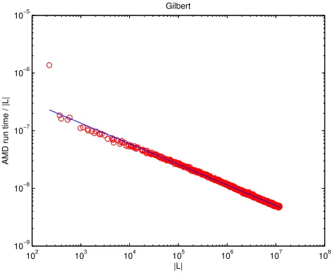
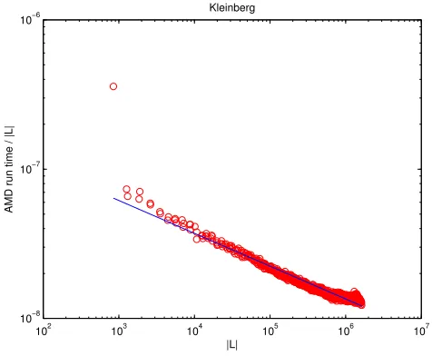
5. COMPUTATIONAL EXPERIMENT
For a brief illustration of the toolbox in use, we follow Davis [Davis 2007] by exam-ining the complexity of the minimum degree ordering algorithm, as implemented
in MATLAB’samd. LettingL denote the Cholesky factor of the appropriate
per-muted version of A, we plot the run time, scaled by |L|, against |L|, on a log-log
scale. Davis [Davis 2007] distinguished between matrices from a deterministic test set coming from problems with and without inherent geometry. To mirror this,
Figure 3 shows results for matrices arising from the Gilbert class, using gilbert,
where there is no inherent structure, and Figure 4 shows results for matrices arising
from the Kleinberg class, using klein, where there is an underlying lattice. The
least-squares slope is indicated by a solid line. In each case the matrix dimensionn
was varied between 50 and 10,000. The test programs are available from the testing section of the toolbox website. The figures are consistent with the rule of thumb
mentioned in [Davis 2007] that the run time is typically belowO(|L|).
6. SUMMARY: NETWORKS AS TEST MATRICES
102 103 104 105 106 107 10−8
10−7 10−6
Kleinberg
|L|
[image:14.612.182.420.72.268.2]AMD run time / |L|
Fig. 4. amdrun times for Kleinberg model
ACKNOWLEDGMENTS
We thank Tim Davis for useful advice about sparse matrix operations in MATLAB.
REFERENCES
Abello, J.,Buchsbaum, A.,and Westbrook, J.1998. A functional approach to external graph algorithms. Lecture Notes in Computer Science 1461, 332–343.
Albert, R. and Barab´asi, A.-L.2002. Statistical mechanics of complex networks. Reviews of Modern Physics 74, 47–97.
Alon, U.2006. An Introduction to Systems Biology. Chapman & Hall/CRC, London.
Anderson, E.,Bai, Z.,Bischof, C.,Blackford, S.,Demmel, J.,Dongarra, J.,Croz, J. D.,
Greenbaum, A.,Hammarling, S.,McKenney, A.,and Sorensen, D.1999.LAPACK Users’ Guide, Third ed. SIAM, PA.
Barab´asi, A.-L. and Albert, R. 1999. Emergence of scaling in random networks. Sci-ence 286,5439, 509–12.
Batagelj, V. and Brandes, U.2005. Efficient generation of large random networks. Phys. Rev. E 71, 036113.
Boginski, V.,Butenko, S.,and Pardalos, P. M.2003. On structural properties of the market graph. InInnovations in Financial and Economic Networks, A. Nagurney, Ed. Edward Elgar Publishers, 29–45.
Boisvert, R.,Pozo, R.,Remington, K.,Barrett, R.,and Dongarra, J.1997. Matrix Market: a web resource for test matrix collections. InThe Quality of Numerical Software: Assessment and Enhancement, R. Boisvert, Ed. Chapman and Hall, London, 125–137.
Bollob´as, B.1985. Random Graphs. Academic, London.
Bollob´as, B.,Riordan, O.,Spencer, J.,and Tusn´ady, G. 2001. The degree sequence of a scale-free random graph process.Random Structures and Algorithms 18, 279–290.
Broder, A.,Kumar, R.,Maghoul, F.,Raghavan, P.,Rajagopalan, S.,Stata, R.,Tomkins, A.,and Wiener, J.2000. Graph structure of the web. Computer Networks 33, 309–320.
·
Conyon, M. J. and Muldoon, M. R.2006. The small world of corporate boards. Journal of Business Finance and Accounting 33, 1321–1343.
Cour, T.,Benezit, F.,and Shi, J.2005. Spectral segmentation with multiscale graph decom-position. In IEEE International Conference on Computer Vision and Pattern Recognition (CVPR). Vol. 2. 1124–1131.
Davis, T.2007. The University of Florida sparse matrix collection. Tech. Rep. CISE Department, REP-2007-298, University of Florida, USA.
de Silva, E. and Stumpf, M.2005. Complex networks and simple models in biology. J. R. Soc. Interface 2, 419–430.
de Silva, E.,Thorne, T.,Ingram, P.,Agrafiot, I.,Swire, J.,Wiuf, C.,and Stumpf, M. P. H.2006. The effects of incomplete protein interaction data on structural and evolutionary inferences. BMC Biology 4:39.
Duff, I. S.,Grimes, R. G.,and Lewis, J. G.1989. Sparse matrix test problems. ACM Trans. Math. Soft. 15, 1–14.
Erd¨os, P. and R´enyi, A.1959. On random graphs. Publ. Math. Debrecen 6, 290–297.
Fagiolo, G.2007. Clustering in complex directed networks. Physical Review 76, 026107.
Faloutsos, M.,Faloutsos, P.,and Faloutsos, C. 1999. On power-law relationships of the internet topology. Computer Communications Review 29, 251–262.
Gilbert, E. N.1959. Random graphs. Ann. Math. Statist. 30, 1141–1144.
Gilbert, J. R.,Moler, C.,and Schreiber, R.1992. Sparse matrices in MATLAB: design and implementation.SIAM J. Matrix Analysis Applications 13, 333–356.
Grimmett, G.1999. Percolation, 2nd ed. Springer.
Grindrod, P.2002. Range-dependent random graphs and their application to modeling large smal-world proteome datasets. Phys. Rev. E 66, 066702.
Grindrod, P.,Higham, D. J.,and Kalna, G.2008. Periodic reordering. Tech. Rep. 6, University of Strathclyde, Department of Mathematics.
Han, J. D. H.,Dupuy, D.,Bertin, N.,Cusick, M. E.,and M., V.2005. Effect of sampling on topology predictions of protein-protein interaction networks.Nature Biotechnology 23, 839–844.
Hendrickson, B. and Leland, R. 1994. The Chaco user’s guide: Version 2.0. Tech. Rep. SAND94–2692, Sandia National Laboratories, Albuquerque.
Higham, D. J.2003. Unravelling small world networks. J. Comp. Appl. Math. 158, 61–74.
Higham, D. J.2005. Spectral reordering of a range-dependent weighted random graph.IMA J. Numer. Anal. 25, 443–457.
Higham, D. J. and Higham, N. J.2000. MATLAB Guide. Society for Industrial and Applied Mathematics, Philadelphia, PA, USA.
Higham, D. J.,Prˇzulj, N.,and Raˇsajski, M.2008. Fitting a geometric graph to a protein-protein interaction network. Bioinformatics 24, 1093–1099.
Hu, Y. and Scott, J. A.2003. HSL_MC73: A fast multilevel Fiedler and profile reduction code. RAL-TR-2003-36, Numerical Analysis Group, Computational Science and Engineering Depart-ment, Rutherford Appleton Laboratory.
Kamper, L., Bozkurt, A., Rybacki, K., Geissler, A., Gerken, I., Stephan, K. E., and K¨otter, R.2002. An introduction to CoCoMac-Online. The online-interface of the primate connectivity database CoCoMac. InNeuroscience Databases A Practical Guide, R. K¨otter, Ed. Kluwer Academic, Norwell, MA, 155–169.
Kauffman, S. A.1969. Metabolic stability and epigenesis in randomly constructed genetic nets.
J. of Theor. Biol. 22, 437–467.
Khanin, R. and Wit, E. 2006. How scale-free are gene networks? Journal of Computational Biology 13,3, 810–818.
Kiss, I. Z.,Green, D. M.,and Kao, R. R.2006. The network of sheep movements within Great Britain: network properties and their implications for infectious disease spread. J. Roy. Soc. Interface 3, 669–677.
Langville, A. N. and Meyer, C. D. 2006. Google’s PageRank and Beyond: The Science of Search Engine Rankings. Princeton University Press, Princeton.
Lov´asz, L.1996. Random walks on graphs: A survey. InPaul Erd¨os is Eighty, D. Mikl´os, V. T. S´os, and T. Sz¨onyi, Eds. J´anos Bolyai Mathematical Society, Budapest, 353–398.
Mangan, S. and Alon, U.2003. Structure and function of the feed-forward loop network motif.
Proc. Nat. Acad. Sci. 100, 11980–11985.
Mangan, S.,Zaslaver, A., and Alon, U.2003. The coherent feedforward loop serves as a sign-sensitive delay element in transcription networks. J. Math. Biol. 334/2, 197–204.
Milenkovic, T.,Lai, J.,and Przulj, N.2008. GraphCrunch: A tool for large network analyses.
BMC Bioinformatics 9:70.
Milgram, S.1967. The small world problem. Psychology Today 2, 60–67.
Milo, R.,Itzkovitz, S.,Kashtan, N.,Levitt, R.,Shen-Orr, S.,Ayzenshtat, I.,Sheffer, M.,
and Alon, U.2004. Superfamilies of evolved and designed networks.Science 303, 1538–1542.
Morrison, J. L., Breitling, R.,Higham, D. J.,and Gilbert, D. R. 2005. Generank: Us-ing search engine technology for the analysis of microarray experiments. BMC Bioinformat-ics 6:233.
Morrison, J. L.,Breitling, R.,Higham, D. J.,and Gilbert, D. R. 2006. A lock-and-key model for protein-protein interactions. Bioinformatics 2, 2012–2019.
Newman, M. E. J.2004. Who is the best connected scientist? a study of scientific coauthorship networks. InComplex Networks, E. Ben-Naim, H. Frauenfelder, and Z. Toroczkai, Eds. Springer, 337–370.
Newman, M. E. J.,Moore, C.,and Watts, D. J.2000. Mean-field solution of the small-world network model. Phys. Rev. Lett. 84, 3201–3204.
Norris, J. R.1997. Markov Chains. Cambridge University Press.
Onody, R. N. and de Castro, P. A.2004. Complex network study of Brazilian soccer players.
Phys. Rev. E 70.
Page, L.,Brin, S.,Motwani, R.,and Winograd, T.1998. The PageRank citation ranking: Bringing order to the web. Tech. rep., Stanford Digital Library Technologies Project.
Penrose, M.2003.Geometric Random Graphs. Oxford Univeristy Press.
Porter, M. A.,Mucha, P. J.,Newman, M. E. J.,and Warmbrand, C. M.2005. A network analysis of committees in the United States House of Representatives.Proc. Nat. Acad. Sci. 102, 7057–7062.
Prˇzulj, N.,Corneil, D. G.,and Jurisica, I.2004. Modeling interactome: Scale-free or geomet-ric? Bioinformatics 20,18, 3508–3515.
Prˇzulj, N.,Corneil, D. G.,and Jurisica, I.2006. Efficient estimation of graphlet frequency distributions in protein-protein interaction networks.Bioinformatics 22, 974–980.
Prˇzulj, N. and Higham, D. J.2006. Modelling protein-protein interaction networks via a stick-iness index. J. Roy. Soc. Interface 3, 711–716.
Salath´e, M.,May, R. M.,and Bonhoeffer, S.2005. The evolution of network topology by selective removal.J. R. Soc. Interface 2, 533–536.
Sporns, O. and Zwi, J. D.2004. The small world of the cerebral cortex. Neuroinformatics 2, 145–162.
Stumpf, M. P. H.,Wiuf, C.,and May, R. M.2005. Subnets of scale-free networks are not scale-free: Sampling properties of networks. Proc. Nat. Acad. Sci. 102, 4221–4224.
Thomas, A., Cannings, R.,Monk, N. A. M.,and Cannings, C.2003. On the structure of protein-protein interaction networks.Biochemical Soc. Tranl. 31, 1491–1496.
Titz, B.,Schlesner, M.,and Uetz, P.2004. What do we learn from high-throughput protein interaction data? Expert Review of Proteomics 1, 111–121.
Watts, D. J. and Strogatz, S. H. 1998. Collective dynamics of ’small-world’ networks. Na-ture 393, 440–442.