City, University of London Institutional Repository
Citation
:
Wang, Y. & Liatsis, P. (2012). 3-D Quantitative Vascular Shape Analysis for
Arterial Bifurcations via Dynamic Tube Fitting. IEEE Transactions on Biomedical
Engineering, 59(7), pp. 1850-1860. doi: 10.1109/TBME.2011.2179654
This is the accepted version of the paper.
This version of the publication may differ from the final published
version.
Permanent repository link:
http://openaccess.city.ac.uk/7743/
Link to published version
:
http://dx.doi.org/10.1109/TBME.2011.2179654
Copyright and reuse:
City Research Online aims to make research
outputs of City, University of London available to a wider audience.
Copyright and Moral Rights remain with the author(s) and/or copyright
holders. URLs from City Research Online may be freely distributed and
linked to.
City Research Online:
http://openaccess.city.ac.uk/
[email protected]
Abstract—Reliable and reproducible estimation of vessel
centrelines and reference surfaces is an important step for the assessment of luminal lesions. Conventional methods are commonly developed for quantitative analysis of the ‘straight’ vessel segments and have limitations in defining the precise location of the centreline and the reference lumen surface for both the main vessel and the side branches in the vicinity of bifurcations. To address this, we propose the estimation of the centreline and the reference surface through the registration of an elliptical cross sectional tube to the desired constituent vessel in each major bifurcation of the arterial tree. The proposed method works directly on the mesh domain, thus alleviating the need for image upsampling, usually required in conventional volume domain approaches. We demonstrate the efficiency and accuracy of the method on both synthetic images and coronary CT angiograms. Experimental results show that the new method is capable of estimating vessel centrelines and reference surfaces with a high degree of agreement to those obtained through manual delineation. The centreline errors are reduced by an average of 62.3% in the regions of the bifurcations, when compared to the results of the initial solution obtained through the use of mesh contraction method.
Index Terms—Bifurcation, Centreline Estimation, CTA,
Coronary Arteries, Elliptic Cross Sections, Shape analysis, Tubular Deformable Model.
I. INTRODUCTION
therosclerosis is a condition where plaques become clogged up in the medium and large arteries of the heart, which could lead to severe consequences, such as heart attack and stroke. Arterial bifurcations, in particular, are prone to developing atherosclerotic lesions because of the turbulent blood flow and the changing shear stress, which accounts for about 20-30% of all percutaneous coronary interventions [1]. Hence, there is a need to develop dedicated techniques to perform reproducible quantification and report the angiographic results for bifurcation lesions.
Fractional flow reserve (FFR), a technique which measures the pressure differences between a stenotic artery and the normal segment proximal to the lesion, is considered to be the golden standard for the diagnosis of myocardial ischemia in clinical practice [2]. However, as it is an invasive procedure, it carries a certain amount of risk in terms of morbidity and
This work was supported in part by City University London through the Y. Wang is with the Information Engineering and Medical Imaging Group, City University, London, UK (e-mail: yin.wang.1@ city.ac.uk).
P. Liatsis is with the Information Engineering and Medical Imaging Group, City University, London, UK (phone: +44(0) 20 7040 8126; fax:+44 (0)20 7040 8568; e-mail: [email protected]).
[image:2.612.342.537.437.537.2]mortality. Recent advances in CT imaging offer a non-invasive alternative for imaging of the coronary artery within one breath-holding. CT produces a 3D volumetric image of the heart with high spatial and temporal resolutions, which allows the construction of patient-specific models of the coronary arteries for the assessment of the severity of arterial stenosis and potentially the means for evaluation of the functional significance of coronary stenoses by carrying out image-based haemodynamic analysis of the blood flow in the arteries [3, 4]. Despite the significant volume of past and on-going research, characterisation of local geometry information in the vicinity of a vessel bifurcation, such as estimation of vessel centrelines and reference surfaces, remains a changeling task, due to the irregular local geometries of the bifurcation. Conventional approaches determine the width of the reference vessel by linear interpolation of the normal vessel parts before and after the bifurcation, however, this does not suffice for reconstruction of the reference vessel in 3D. To characterise the morphology of the bifurcation, a closed surface representing the reference vessel’s boundaries is required, as it would further support the choice of treatment and analysis of the geometric changes which may occur following coronary intervention [5].
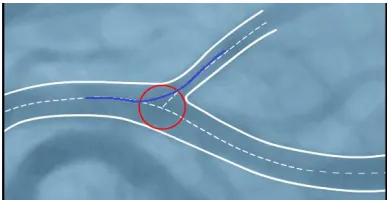
Fig. 1. The synthetic image illustrates the vessel centrelines defined based on the locus of the maximal circles/spheres within the vasculature. It shows that the detected centreline (dashed curves) deviates from the manually delineated one (shown in blue colour) near the bifurcation region.
Li and Yezzi [6] modelled the vascular structure as a 4D curve (centreline coordinates and vessel radius) and proposed the use of a minimal path based method to simultaneously detect the vessel surface and determine the centreline between two manually selected seed points. Along the same research direction, Antiga et al. [7] proposed the extraction of centrelines by finding the locus of centres of maximal spheres inscribed into the tubular structures based on the Voronoi diagram of the object’s surface points. Both methods, however, are only able to correctly estimate the centrelines of single branch vessels. Inaccurate estimation may occur in the presence of multiple branching structures (e.g., vessel bifurcations) as
3D Quantitative Vascular Shape Analysis for
Arterial Bifurcations via Dynamic Tube Fitting
Yin Wang and Panos Liatsis,
Member, IEEE
the centreline cannot be precisely defined by using the centre of the maximally embedded sphere in the bifurcation area. Fig. 1 illustrates the problematic centrelines defined in the vicinity of a bifurcation using 4D curve based algorithms.
Deformable model based methods have been widely used in modelling of vascular structures. Such methods allow the local deformation of a curve (surface) in terms of image features, while maintaining global smoothness, usually constrained by inherent physical characteristics, such as elasticity and stiffness. Wong and Chung [8] proposed a deformable tube model based method to recover the healthy shape of abnormal vessels in 3D angiography images. In their method, the original shape of a diseased vessel segment is reconstructed by registering a circular cross sectional tube to the vessel boundaries in the normal regions. However, their method is sensitive to initialisation, since the widths along the tube are determined by linear interpolation between two manually selected cross sections. This may lead to under- or over-estimation of the area of tube cross sections due to the non-linear nature of the vessel, thus resulting in erroneous estimation of vessel centrelines and the reference surface. In addition, the tube deformation process is carried out in the voxel domain, which requires upsampling of the original volume to calculate the image-based energy in the case of insufficient resolution. However, the choice of the image upsampling technique could dramatically affect the magnitude of the image-driven energy, leading to non-unique solutions for the tube registration problem. Similar work was also reported in Kang et al. [9], who proposed the classification of the region of interest (ROI) to one of three types, namely, normal, stenotic and aneurismal (corresponding to bifurcations), prior to model registration. In a departure from previous methods, which define vessel cross sections by finding the perpendicular plane to the tangent direction of the centreline at each point, they propose the determination of vessel cross sections by extracting the isosurface from the complementary geodesic distance field, which permits the cross sections of the tube to be determined uniquely and independently of the fitted centrelines. In this method, the classification of the ROI is based on the segmented image, which is obtained using a region-growing algorithm. The ‘leakage problem’, which is commonly encountered in region-growing based segmentation, however, could result in erratic classification of the ROI and subsequently degrade the performance of the method.
The current work introduces an automated algorithm for simultaneous determination of centrelines and reference surfaces in coronary bifurcations. The proposed algorithm is based on the concept of deformable tube registration, and offers a number of advantages compared to previous approaches. Firstly, it works directly on the mesh domain, which alleviates the requirement for image upsampling. Secondly, contrary to conventional circular cross sectional tube models [8-10], which use linear interpolation to determine the width along the tube, the proposed method estimates the tubular cross sections based on partial information of the vessel surface to be fitted. Specifically, the cross sections of the tube are adaptively estimated by finding the best fitting ellipse to the intersection
points (obtained by slicing the vessel surface using a cutting plane which is perpendicular to the centreline points) belonging to the desired constituent branch of the bifurcation. Thirdly, a weighted directional distance metric is employed to measure the goodness of the fit between the tube and the vessel of interest in the energy calculation, which facilitates tube registration at the desired location of the bifurcation. In addition, we propose the use of a hybrid optimisation method to minimise the tube energy functional. In particular, a local greedy search is used to determine the initial solutions for the relevant vessel locations, which are then optimised using dynamic programming (DP). The proposed optimisation strategy ensures the global optimality of the solution, and permits the incorporation of hard constraints, posed on the tube within a natural and direct framework.
The remainder of the paper is organised as follows. In Section II, we describe the proposed method in detail. This is followed by the presentation and analysis of the results, which demonstrate the performance of the approach in terms of efficiency and accuracy. Finally, Section IV is dedicated to the conclusions of the research and a discussion of possible future directions.
II. METHODS
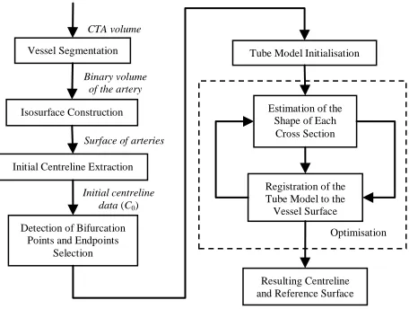
The purpose of this research is to develop a methodology for the extraction of an anatomically valid centreline and the determination of the corresponding reference surface in arterial bifurcations. It is assumed that the stage of vessel segmentation has been previously completed and the segmented vessel volume set is available prior to the tube registration. Without loss of generality, a binary image volume, with voxels labelled to one for vessels and zero for others, is used to represent the vessel segmentation. The coronary arteries are extracted using a generalised active contours algorithm, described in previous work [11]. The binary volume is then converted to its equivalent mesh domain by finding the zero-isosurface using the marching cube algorithm [12]. The flow chart of the proposed approach is shown in Fig. 2. It commences with the extraction of the initial centreline location of the arterial trees, by using the mesh contraction algorithm [13]. The resulting centreline data, C0, are represented by two arrays, holding the
coordinates of the centreline points (nodes) and the sets of indices, which define the adjacent points for each node, respectively. Based on the initial centreline (C0), bifurcation
considered as the resulting centreline for each of the constituent vessel segments of the bifurcation, and the tube surface can be used as the reference vessel.
[image:4.612.65.293.98.270.2]
Fig. 2. Flow chart of the proposed framework.
A. Explicit Vascular Model
1) Deformable Tube Model: The proposed tube model, R(v,θ), is defined in terms of its central axis and the corresponding cross sections. The points v={vi, i=1,…,N}
represent the path of the N control points (moving nodes), where N is adaptively chosen to ensure the distance between adjacent moving nodes is less than 0.5 voxels, and θ={i,,
i=1,…,N} is an array consisting of the parameters of the associated cross sections. In this research, the cross section of the tube model is approximated as the best fitting ellipse. Hence, at the i-th moving node vi, the parameter vector is
defined as θi={ai,bi,u1i,u2i,φi}, where ai and bi represent the semi
diameters of the axes of the ellipse, u1i,and u2idenote the origin
of the ellipse, and φiis the tilt angle. The central axis of the tube
is defined using a B-spline curve with N moving nodes, and the surface of the tube can be reconstructed from its circumferences (i.e., the cross sections along its centreline) by using the ball pivoting algorithm [14].
The tube registration problem is solved by minimising a generic active contour energy functional, defined as follows:
E
E
Int
E
Ext
E
Con (1)where η and γ are constants, controlling the influence of each energy term on the total tube energy. The internal energy, EInt,
is comprised of the elasticity (v´(s)=dv/ds, where v(s) represents the medial axis and s is the arc length parameter) and the stiffness of the medial axis (v´´(s)=d2v/ds2):
s
v
s
v
s
d
s
E
Int(
|
'
(
)
|
2
|
''
(
)
|
2)
(2) The constants α and β are the weights for the elasticity and stiffness, respectively.The external energy functional, EExt, is derived from the
fitting error between the tube model and the desired vessel segment. This poses a strong constraint on the tube based on its position with respect to the vessel surface, making the tube
deform and follow the course of the vessel of interest. In this research, we define the external energy of the tube as follows:
s
Ext
F
ds
E
(
v
(
s
),
θ
)
(3)where F(v(s),θ) is a scalar function, returning the similarity score between the tube model and the desired branch. The metric is defined as the weighted directional distance between the fitting tube and the vessel surface, which will be discussed later on in Section II-B.
The elastic force defined in the internal energy favours small distances between adjacent centreline points, which will eventually shrink the curve to a single point. To prevent shrinking, an additional constraint, which encourages equal spacing between the centreline points, is defined as follows:
E
Con
d
(
v
(
s
))
d
2 (4)where d(v(s)) denotes the distance between the control point v(s) and its successive neighbour along the centreline, and d is the average distance between the centreline points.
B. Construction of the Reference Surface
In this research, the reference surface for each constituent branch of a bifurcation is constructed through the registration of a deformable tube model to the desired branch. In contrast to conventional tubular models using fixed cross sections, the proposed approach adaptively updates the shape of the tube model, thus resulting in a more robust and accurate estimation. To this end, the method alternates between updating the cross sectional shape of the tube and registering the tube model to the desired branch.
1) Estimation of the Shape of each Cross Section: The circular cross sectional tube is the most popular model to approximate vascular structures in the literature. Vessels, however, are elastic bodies, which can accommodate local deformations of the lumen due to changes in blood flow and intraluminal pressure within the artery. Such deformations cannot be accurately represented using circular cross sections. Hence, we use an elliptical cross sectional tube model to approximate the vessel surface, which provides sufficient degrees of freedom to accommodate the potential deformations and facilitates the accurate estimation of the vessel cross sections. An ellipse can be defined in parametric form as:
x
u
Q
(
)
x
'
(5)where,
cos sin
sin cos ) ( , sin cos ' , ) ,
( 1 2 Q
t b
t a u
u T x u
xdenotes a point located on the circumference of the ellipse, u is the centre of the ellipse, a and b represent the semi-lengths of its axes, φ denotes the tilt angle, i.e., the angle between the x-axis of the local coordinate system and the major axis of the ellipse, and t is an angular parameter varying between 0 to 2π. The minimum distance of an arbitrary point, p= [p1, p2]T, to the
circumference of the ellipse can be found by:
Optimisation
Initial centreline data (C0) Surface of arteries Binary volume
of the artery CTA volume
Tube Model Initialisation
Isosurface Construction
Detection of Bifurcation Points and Endpoints
Selection
Registration of the Tube Model to the Vessel Surface Estimation of the
Shape of Each Cross Section
Resulting Centreline and Reference Surface Vessel Segmentation
2 2 1 2 1 2 sin cos ) ( | | min t b t a Q u u p p d
t p x
(6)
Let Pi= [(p11, p12), (p21, p22), ..., (pm1, pm2)] T, (m>U, where U≥5
with the lower value representing the number of free parameters of the ellipse) to be the intersection points, found by slicing the vessel surface using a perpendicular plane at the location of each moving node. The best fit ellipse, for which the sum of the squares of the distances to the given points is minimum, can be found by solving the following nonlinear least squares problem [15]:
min sin cos ) ( 1 2 2 1 2 1
m j j j j j t b t a Q u u p p (7)
In order to produce a smooth and anatomically correct generalisation of the tube model, we further constrain the area of the fitting ellipse, by limiting the lengths of its axes, based on its neighbouring slices. Specifically, we restrict the length of the axes of the ellipse to lie in the range of [1-c, 1+c] with respect to its adjacent cross sections. The constant c (fixed to 0.2) is determined based on the viscoelastic properties of the vessel in [16], where the authors conducted a series of in vitro experiments to validate the ability of their CFD model in simulating blood flow within the vessel by considering the deformation of the vessel wall.
Let τ= [t1,…, tm, a, b, u1, u2, φ]T denote the unknown
parameters which need to be determined. By taking into consideration the constraints imposed on the axes of the ellipse, we set up with the constrained nonlinear least squares problem as follows: W τ τ A sin cos ) ( min 2 2 1 2 1 to subject t b t a Q u u p p j j j j (8) where 1 1 1 1 2 . 1 8 . 0 2 . 1 0.8 0 0 0 1 0 0 0 0 0 0 1 0 0 0 0 0 0 0 1 0 0 0 0 0 0 1 0 0 i i i i m b b a a ... ... -... ... A W
The subscript i denotes the i-th moving node along the central axis of the tube model.
2) Computation of the Tube Energy: By discretising the energy functional defined in (1), the tube energy can be rewritten as:
( , , ) ( ) ( ) ( )
1
1 Con i
N i i Ext i Int N
Total E E E
E ν ν
ν
ν
ν
(9)
where 2 2 1 2 1 1 2 1 | |) (| | ) ( | 2 | | | d E , F E E i i Con i i Ext i i i i i Int v v θ v v v v v v (10) and
N i i i N d 2 2 1| | 1 1 v vHere, vi denotes the moving node of the tube centreline, and the
external energy is calculated by F(vi,θi), which returns the
weighted sum of squared errors between the estimated cross sections θi and the vessel boundaries intersected by the cross
section at the location of the moving node vi. Due to the
irregular geometry of the vessel cross sections at the location of the bifurcation, as shown in Fig. 3, not all of the intersection points belong to the desired branch, rather a subset of the intersection points may belong to another vessel branch. Hence, modelling the tube cross sections using all of the intersection points may introduce inaccuracies in defining the reference vessel surface. To address this issue, we make use of directional information to measure the difference between the model and the vessel boundaries, where the intersection points belonging to the desired vessel surface are assigned higher weights.
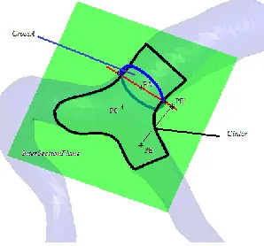
A vessel bifurcation is defined as the subdivision of a vessel into two branches. As depicted in Fig. 4(a), it can be considered as a single object delineated by a left, middle and right contour, respectively [17]. In Fig. 4(b), we extend this concept to 3D images, where a bifurcation comprises three surfaces, namely the left, middle and right surfaces, respectively. As an example, let us consider the vessel segments shown in Fig. 3(a), the objective being to fit the tube model to the distal main branch (the right branch) over the bifurcation. To this end, the tube surface needs to be accurately registered onto the right surface of the vessel, as its left counterpart belongs to another constituent vessel of the bifurcation. However, it should be noted that, the terms ‘left’ and ‘right’ surface are ambiguous in 3D space, as the definitions of ‘left’ and ‘right’ are relative to the viewpoint. In order to correctly register the tube model onto the desired surface, we propose a viewpoint-independent procedure to determine the surface of interest in an automated fashion. As illustrated in Fig. 5, we firstly find the intersection curve (Cinter, shown in black) between the vessel surface and the
intersection plane (i.e., the green plane), defined by the two endpoints (PA and PB) together with the bifurcation point (PC), in the vicinity of the bifurcation area. Then, the orientation of the x-axis of the cross section at PA (denoted by CrossA) coincides with the direction of the line segment (shown in red), defined as the intersection between the plane CrossA and the curve Cinter. Next, we project the endpoint PB onto the plane
vice versa. In order to deal with the torsion of 3D vessels, the technique of rotation minimising frames [18] is employed to determine the local reference frame for each point of the centreline axis of the tube. Based on the local frame, we define the directionalweights as:
)
2 ) ( exp( 2
1
2 2
2
w (11)
where is an angular parameter as illustrated in Fig. 6(a), φ is the tilt angle of the estimated ellipse at the current cross section, and σ indicates the variance of the normal distribution, which is chosen to be equal to 60 degrees [(see Fig. 6(b)). The weights assigned for fitting the left and right surfaces are shown in Figs. 6(c) and (d), respectively.
[image:6.612.316.553.124.331.2](a) (b)
Fig. 3. Illustration of the intersection points taken from the vessel bifurcation. (a) The 3D view shows the intersection points in the vicinity of the vessel bifurcation. (b) The intersected points of (a) shown in a 2D projection image. The black dots are the vessel boundary points, while the red dot is the position of the centreline point at the cross section. Points on the right side of the centreline location are parts of the right surface, and exhibit normal vessel shape. Their left hand side counterparts belong to the side branch of the bifurcation, and are characterised by an irregular shape.
[image:6.612.63.289.228.332.2]
(a) (b)
Fig. 4. Representation of the vessel bifurcation in (a) 2D, and (b) 3D, respectively. The vessel bifurcation is treated as a single segment delineated by three contours/surfaces.
Fig. 5. Illustration of the proposed scheme for the determination of the desired surface. The semi-transparency structure represents the vessel surface.
The intersection plane, defined by the endpoints PA and PB together with the bifurcation point PC, is shown in green. The black curve depicts the intersection curve between the plane and the vessel surface near the bifurcation. The cross section taken at endpoint PA, denoted by CrossA, is delineated by the blue contour, and the red line shows the x-axis direction of the cross section at PA.
(a) (b)
[image:6.612.65.283.422.519.2](c) (d)
Fig. 6. The directional weights scheme used in the registration of the tube to the desired surface in the bifurcation. (a) The definition of the angular coordinate system. (b) The weight distribution as a function of the angle, when fitting the right hand side surface. (c) and (d) 3D plots of the distribution of weights for the left and right surfaces, respectively. The estimated cross section is shown in blue and the height of the plot at each point indicates the relative magnitude of the weights.
Given the parameter vector of the cross sectional model θi={ai,bi,u1i,u2i,φi}, i.e., the best fit ellipse approximating the
cross sectional shape of the vessel at the i-th moving node, and the directional weights, the goodness of the fit for each cross section at the moving node xi can be expressed as:
}
sin cos ) ( {
min ) , (
2
2 1
2 1
1
j
j
i i
j j j g
j t i i
t b
t a Q u u p p w F
j
θ
x (12)
where P = {(pj1, pj2), j=1,...,g}, denote the intersection points as
defined in the previous section, wjis the weight associated with
the direction tj, and g denotes the number of points on the
intersection.
[image:6.612.85.234.572.711.2]lowest energy in the search space, are firstly determined using an exhaustive search algorithm [19]. The node energies are obtained by the sum of the individual energy functions as defined in (10). The search space is defined as a four voxels width square grid with a step size of 0.2 voxels, perpendicular to the tangential direction of the centreline at each moving node. Next, dynamic programming is applied to determine the global optimal path of the centreline among all possible paths connecting the suboptimal solutions. In this paper, we follow the terminology and notation of the work of Amini et al. [20], and the tube energy is then expressed as the sum of triple-interaction potentials as follows:
) , , ( ) , , ( ) , , ( ) , , ( ) , , ( 1 2 2 4 3 2 2 3 2 1 1 1 2 1 1 1 1 N N N N N i i i i i N Total E E E E E v v v v v v v v v ν ν ν ν ν
(13) where
E
i1(
v
i1,
v
i,
v
i1)
E
Ext(
v
i)
E
Int(
v
i)
E
Con(
v
i)
(14)In general, dynamic programming is a serial multistage decision process, which decomposes a problem as a number of single stage processes, connected in series. The solution of the dynamic programming involves the determination of a sequence of optimal value functions (Si(vi+1,vi), i=1,...,N) for
each stage. The optimal value function is defined by two adjacent moving nodes on the centreline as:
(
,
)
min
{
(
,
)
(
,
,
)}
1 1 1 1 1 1 1
i i i i i i i
i i
i
S
E
S
iv
v
v
v
v
v
v
v (15)where the moving node vi serves as the state variable in the i-th
decision stage and is only allowed to move on the discrete grid within the search space. For fixed values of vi and vi+1, the value
of the function Si(vi+1,vi) is determined by finding the minimum
value of the right-hand side of (15), when moving the node vi-1
over the space of its possible positions. In each decision stage, the optimal value function incorporates information from three successive moving nodes, and hence, the global optimal solution can be obtained recursively in terms of the consecutive nodes on the centreline.
III. EXPERIMENTAL RESULTS AND ANALYSIS
In this section, we apply our method to both synthetic and clinical images to demonstrate the efficiency and accuracy of the proposed method in defining the centreline and reference vessel surface over the vessel bifurcation. We firstly compare the proposed image-driven energy functional with its volume domain counterparts, i.e., Wong and Chung’s method [8] and the model proposed by Kang et al. [9], to show the benefits offered by the proposed energy formulation. The comparison was carried out using synthetic 3D vascular images, which allow testing these energy metrics on various types of vessel segments with known optimal solutions (i.e., ground truth data). Next, we validate our method in clinical CTA images and compare its performance against the approach reported by Antiga et al., in the determination of the centreline location in
vessel bifurcations.
A. Experiments on Synthetic Images
The synthetic tubes were generated using the locus of the central axis and associated cross sections (for simplicity, the circular cross sectional tube model was used). The tubes were represented by a binary volume, in both the mesh and volume domains. Fig. 7 illustrates an example of a synthetic tubular image.
Since the purpose of this experiment is to compare the performance of the aforementioned image-driven energies in measuring the fitness of the tube model at bifurcation areas, the central axis of the tube model was initialised using the optimal solution for all of the methods. In terms of the associated cross sections, they are determined by linear interpolation between two ending cross sections, located prior and distal to the bifurcation, for both Wong and Chung’s and Kang et al. methods. We follow the procedure described in Section II-B to estimate the cross sections for the proposed tube model.
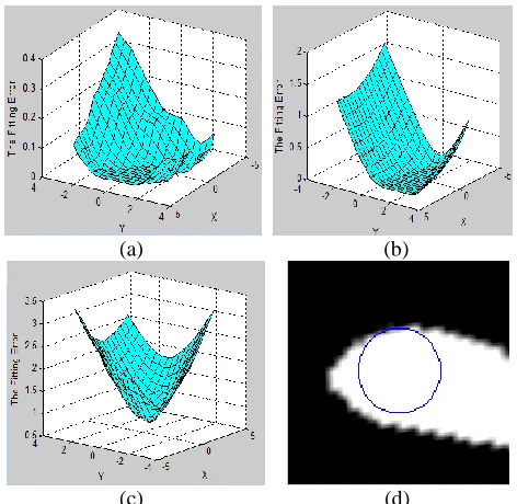
Fig. 8 depicts the change of magnitude of the image-driven energies with respect to the distance of the control point from the optimal position at the bifurcation area. In this experiment, the control point is only allowed to move on a square grid, perpendicular to the tube centreline at each control point. The radius of the grid was set to three voxels, and the grid size was chosen to be 0.2 voxels. Linear interpolation was applied for image upsampling in the calculation of the image energies for the volume domain methods. It can be seen from Fig. 8 that both Wong and Chung’s metric (Fig. 8(a)) and image-based energy designed by Kang et al. (Fig. 8(b)) have a flatten region near the optimal location. This is due to the fact that both image-driven energies are based on the degree of overlapping between the tube model and the vessel segment. At a vessel bifurcation, the cross section of the vessel, as shown in Fig. 8(d), deviates from being circular, and thus, the same fitting error will be found when the cross section of the tube model is located within the interior of the vessel area. In this case, the internal energy of the tube model becomes the dominant contributor in these two methods in the vicinity of bifurcations, and thus, the location of the tube is almost entirely determined by this energy term. This may result to erroneous estimation of the reference surface and vessel centrelines, since the internal energy favours a ‘straight’ tube. On the contrary, only a small number of local minima were identified around the optimal position in the proposed image-driven energy formulation.As shown in Fig. 8(c), our image-driven energy generally increases with the distance from the optimal position. Therefore, the proposed model is capable of producing accurate estimation of vessel centrelines and the reference surface.
shown in Fig. 7(b), and the width of the cross section was set to its optimal value. It can be observed from Table I that Wong and Chung’s image-based energy varies in the range of 0.0043 to 0.2083, for different interpolation methods. The maximum value is almost 50 times greater than the minimum, indicating that their method is sensitive to the choice of interpolation scheme. In addition, image upsampling is a computationally expensive operation with the 3D linear interpolation taking approximately 0.4s, while the proposed image energy can be calculated within 3ms for the same cross section.
(a) (b)
Fig. 7. An example illustrating a synthetic tube image. (a) The volume of the tube, and (b) An example of the cross sectional image of the tube (at the location of the green plane in (a) represented in the voxel domain. Voxels labelled as one correspond to the tube while zero is used for the background (linear interpolation was applied to increase the resolution).
(a) (b)
[image:8.612.50.286.175.282.2]
(c) (d)
Fig. 8. Calculation of image-based energies near the vessel bifurcation using various methods. The change in the magnitude of image energies with respect to the distance of the moving node from the optimal solution at the bifurcation area, (a) Wong and Chung’s energy, (b) Kang et al. energy, and (c) The proposed image energy, (d) A cross sectional image of the vessel taken from the bifurcation area. Voxels labelled as one represent the vessel area, and the cross section of the tube model is delineated in blue.
TABLE I
EFFECT OF INTERPOLATION METHODS ON IMAGE ENERGY
Interpolation
Method Wong and Chung’s Energy [8]
Kang et al. Energy [9] Nearest neighbour 0.2083 0.1773
Linear 0.0727 0.1600 Cubic 0.0275 0.1629 Cubic spline 0.0043 0.1501
B. Experiments on Real Clinical Images
Eight coronary CT volumes were acquired from St Thomas and Guys Hospitals, London, UK. Two were imaged with a 16-slice CT scanner (Brilliance, Philips), and the remaining six volumes were acquired with a Philips ICT-256 workstation. In addition, a further four coronary CT studies were obtained from a public database [21]. The mean size of the images is 512 ×512 × 285 with an average in-plane resolution of 0.40 mm × 0.40 mm, and the mean voxel size in the z-axis is 0.42 mm. For each CTA image, four major bifurcations in the main arterial branches, i.e., right coronary artery (RCA), left anterior descending artery (LAD), left circumflex artery (LCX), and one large side branch of the coronaries, were chosen for evaluation. The ground truth centrelines were provided by our clinical collaborators at St Thomas and Guys’ hospitals. Three experts manually and independently annotated the centrelines of the CTA data. They were also asked to specify the radius of the lumen at the centreline points with a sampling of 3mm. The ground truth data (CTR), for which the sum of squares of the
distances to the experts’ delineations is minimal, was determined by solving the associated least square problem. The standard deviation of the centreline CTR was found to be
0.218mm (approximately 0.544 voxels). The tuning parameters of the proposed technique were empirically determined from the training set, which consisted of three CT studies randomly selected from the 12 volumetric datasets. The parameter settings are listed in Table II, and were fixed throughout the experiments.
To quantify the accuracy of the fitting results, two distance metrics, namely, the Mean Square Error (MSE) between the ground truth centreline data and the central axis of the fitting tube, and the MSE between the fitting tube surface and the vessel boundaries, are used to validate the performance of the algorithms.
TABLE II
PARAMETER SETTINGS FOR THE PROPOSED METHOD
Maximum number of iterations, iter 20 Number of suboptimal solutions for each node, Num 10 Elasticity weight, α 0.2 Stiffness weight, β 0.2 Constrained energy weight, γ 0.15 Appearance energy weight, η 1 Axis constraint, c 0.2 Radius of the search space, rad 4 Grid size of the search space, ds 0.2 Maximum number of iterations, emax 100 Stopping criterion, eps 10-6 Circularity criterion for selection of endpoints, comp 0.9
[image:8.612.55.291.339.569.2]constraint becomes the major contributor to the total energy, thus resulting in a ‘straight’ tube, as shown in Fig. 9(b).
The search space of the proposed method is defined as a square grid, given by the window’s radius (rad) and the step size (ds), centred at each moving point along the centreline. We use the vessel segment of Fig. 3(a) to evaluate the performance of the tube fitting process with respect to the rad and ds parameters. It can be seen in Fig. 10(a) that the results change dramatically as the search space step ds increases. This is because a small step size for the search space (i.e, finer resolution) allows a larger number of alternative locations for the node to move and thus improves the overall performance. Large values for the step size (i.e., coarser resolution), however, may result in the node making large and potentially erratic movements On the other hand, the influence of parameter rad, as shown in Fig. 10(b), is not as significant, since the minimum value of the local energy for each node is usually found within a small distance from its initial position. In theory, the choice of parameter rad should not introduce significant changes on the results. However, this parameter still needs to be chosen at the appropriate scale, with the optimal value being the width of the vessel, at the vessel bifurcation. The reason for this is that a large value for the parameter rad can increase the probability for an erroneous movement of the centreline and subsequently increase the computational cost of the optimisation procedure. Since the initial centreline is already near the optimal position, we set the radius of the search space to four voxels in order to improve the efficiency of the proposed algorithm.
[image:9.612.328.549.206.414.2](a) (b)
Fig. 9. The tube centreline obtained by using extreme values for the weights of the smoothness constraints. The tube centrelines obtained by using the standard parameter settings, listed in Table II, are shown in red. The black curves are the centrelines obtained with (a) low, and (b) high weights for the smoothness (stiffness) parameter β.
(a) (b)
Fig. 10. Comparison of the tube fitting results in terms of the centreline and surface fitting errors. Plots (a) and (b) correspond to the influence of parameters
ds and rad, respectively. The centreline fitting error is depicted with the dashed line, while the surface fitting error is illustrated by solid lines.
Fig. 11 illustrates the results obtained from the application of
the proposed method on four clinical datasets, where the semi-transparent structures (shown in blue) are the arterial lumen surfaces, obtained from the vessel segmentation, and the initial centrelines (C0) are shown in blue. The central axis of the
fitting tube is delineated in red, while the corresponding surface is represented in black. Fig. 11(a) shows the fitting of the proposed tube model on the main vessel in the bifurcation. Fig. 11(b) illustrates the registration of the fitting tube onto a highly curved side branch. Fig. 11(c) depicts the result obtained in the neighbourhood of a complex bifurcation, while the ability of our method in fitting a tapering vessel is demonstrated in Fig. 11(d).
(a) (b)
(c) (d)
[image:9.612.58.288.399.492.2]Fig. 11. Tube registration/fitting results obtained from major bifurcations of coronary arteries: (a) Main vessel in a bifurcation (b) A highly curved side branch, (c) A complex bifurcation and and (d) A tapering vessel. The semi transparent structure represents the vessel surface (blue surface). The fitting tube is represented by its central axis (in red) and the outer surface (in black) reconstructed from the cross sections. The blue line denotes the initial centreline estimations.
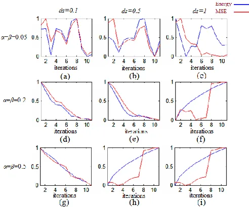
[image:9.612.49.295.557.677.2]process, when the tube energy stops decreasing.
Fig. 12. Correlation between the tube energy and the MSE of the centreline for different parameter settings. The x-axis of the plot corresponds to the number of iterations, while the y-axis corresponds to the normalised MSE and tube energy values. The tube energy and MSE are plotted in blue and red colours, respectively. Plots (a)-(c) show the MSE and tube energy with parameters
rad=2, α=β=0.05, ds={0.1, 0.5, 1}, respectively, plots (d)-(f) for rad=2,
α=β=0.2, ds={0.1, 0.5, 1}, and plots (g)-(f) for parameters rad=2, α=β=0.5,
ds={0.1, 0.5, 1}, respectively.
We also compared the performance of the proposed method using two tube models, i.e., both circular and elliptical cross sectional tubes, with the centreline extraction algorithm reported by Antiga et al. [7], in the determination of vessel centrelines near bifurcations. For the circular cross sectional model, we initialise the tube in a similar way as in Wong and Chung’s method, where the central axis of the tube is defined as the initial centreline of the arteries and the corresponding width of the cross sections along the centreline is determined by linear interpolation between the diameters estimated at the two endpoints. The tuning parameters for the circular cross sectional tube were determined in the case of the elliptical tube, with the help of the same training set. The VMTK toolkit [22] was used to perform the centreline extraction algorithm in [7], and 3D slicer [23] was employed to interactively select the end points for each vessel segment.
As can be observed in Fig. 13, the average MSE of the initial centrelines (C0) near the bifurcation is approximately 1.71
voxels. The error can be reduced by 36% on average with the use of the method proposed in [7] (the MSE was found at 1.05 voxels). For the proposed algorithm, the circular cross sectional tube has a similar performance to Antiga et al. method, where the mean MSE across the test datasets was 0.92 voxels. A further improvement in performance is achieved (i.e., the MSE is reduced by 62.3 % on average compared with the initial centrelines), when using the elliptical cross section tube model. The box and whisker plots of the centreline fitting errors of these models for the eight datasets are presented in Fig. 14. It can be seen that the dispersion of the centreline fitting errors when using the elliptical cross section tube model is the least. This indicates that the proposed elliptical cross section tube
[image:10.612.344.537.158.303.2]model has a higher degree of reproducibility and is more insensitive to the characteristics of the input datasets. The maximum fitting error of our method, when using the elliptical cross section tube model, was found to be equal to 0.86 voxels, which implies that the proposed model is able to estimate the locations of the centrelines over the region of the bifurcation with sub-voxel accuracy. Note that datasets #1-#3 were used as the training set for tuning parameters for all the methods.
Fig. 13. Comparison of the centrelines extracted at the vicinity of the bifurcations using various methods.
Fig. 14. Centreline fitting errors for the clinical datasets obtained using the various models.
The proposed approach was implemented in MATLAB (R2010b) on a standard specification PC (Dell Precision T3500, Inter(R) Xeon(R) CPU at 2.67GHz), and the average execution time was found to be 61.3 seconds for fitting each constituent branch of a bifurcation. VMTK, on the other hand, requires roughly 100s to carry out the same process (when implemented using 3D slicer).
IV. CONCLUSIONS
[image:10.612.349.530.343.485.2]during the registration process. The proposed model directly works on the mesh domain, which eliminates the need for image upsampling, normally encountered in conventional volume domain based methods, in the case of insufficient image resolution. Furthermore, we propose the application of a hybrid optimisation scheme, combining greedy search and dynamic programming, to solve the tube registration problem, which guarantees the global optimality of the solution and allows the enforcement of hard constraints in a natural manner. The efficiency of our method was demonstrated on both synthetic and clinical datasets, with encouraging results. Experiments on synthetic tube images have shown that the proposed image-driven energy is more efficient and accurate in measuring the fitness of the tube model at bifurcation areas. For the real clinical data, the proposed method can produce smooth and morphologically correct centrelines and reference surfaces for both the main vessel and the side branch in the region of a bifurcation. The fitting results show that the proposed method leads to an improvement of 62.3% in accuracy (on average), when compared to the initial centreline locations, obtained through the use of mesh contraction algorithm. The application of the proposed tube model allows for the local geometric parameters of vessel bifurcations to be easily and robustly estimated, which in turn can be used as a starting point for further clinically relevant research. For instance, prediction of the optimal size of a stent is important in intervention treatment, and requires reliable measurement of the centreline length and the distal cross sectional diameters of the vessel segment [24]. Experimental results have shown that vessel centrelines obtained through the proposed technique have a high degree of agreement with the manually delineated ground truth data in the vicinity of bifurcations. Hence, the proposed technique may potentially facilitate for a more accurate prediction of the size of stent. In addition, the proposed system is fully automatic, which supports the estimation of bifurcation geometries with minimal user interaction. Finally, the outputs of this work may be particularly useful in the study of the relationship between local geometries and the associated risk of developing arterial lesions by carrying out patent-specific haemodynamic analysis of the blood flow in the artery [25].
ACKNOWLEDGMENTS
The authors would like to acknowledge Dr Gerry Carr-White and Rebecca Preston at St Thomas and Guys Hospitals for their invaluable advice and the provision of the CTA datasets, and the four anonymous referees for their constructive comments, which have significantly improved the paper.
REFERENCES
[1] K. Samin, J. Sweeny, and A. S. Kini, "Coronary Bifurcation Lesions: A Current Updata," Cardiology Clinics, vol. 28, pp. 55-70, 2010. [2] B. Brueren, et al., "How good are experienced cardiologists at predicting
the hemodynamic severity of coronary stenoses when taking fractional flow reserve as the gold standard.," International Journal of Cardiovascular Imaging, vol. 18, pp. 73-76, 2002.
[3] S. W. Lee, L. Antiga, D. Spence, and D. Steinman, "Geometry of the carotid bifurcation predicts its exposure to disturbed flow," Stroke, vol. 39, pp. 2341-2347, 2008.
[4] G. D. Santis, et al., "Patient specific computational fluid dynamics: structured mesh generation from coronary angiography," Medical and Biological Engineering and Computing, vol. 48, pp. 371-380, 2010. [5] D. Dvir, H. Marom, A. Assali, and R. Kornowski, "Bifurcation lesions in
the coronary arteries: early experience with a novel 3-dimensional imaging and quantitative analysis before and after stenting,"
EuroIntervention, vol. 3, pp. 95-99, 2007.
[6] H. Li and A. Yezzi, "Vessels as 4-D Curves: Global Minimal 4-D Paths to Extract 3-D Tubular Surfaces and Centerlines " IEEE Transacations on Biomedical Engineering, vol. 26, pp. 1213-1223, 2007.
[7] L. Antiga, B. Ene-Iordache, and A. Remuzzi, "Centerline Computation and Geometric Analysis of Branching Tubular Surfaces With Application to Blood Vessel Modeling," in The11th International Conference in Central Europe on Computer Graphics, Visualization and Computer Vision 2003, Campus Bory, Plzen - Bory, Czech Republic, 2004. [8] W. C. K. Wong and A. C. S. Chung, "Augmented Vessel for Quantitative
Analysis of Vascular Abnormalities and Endovascular Treatment Planning," IEEE Transacations on Medical Imaging, vol. 25, pp. 665-684, 2006.
[9] D. G. Kang, D. C. Suh, and J. B. Ra, "Three dimensional Blood Vessel Quantification via Centerline Deformation," IEEE Transacations on Medical Imaging, vol. 28, pp. 405-414, 2009.
[10] D. Craiem, et al., "Coronary Arteries Simplified with 3D Cylinders to Assess True Bifurcation Angles in Atherosclerotic Patients,"
Cardiovascular Engineering, vol. 9, pp. 127-133, 2009.
[11] Y. Wang and P. Liatsis, "An Automated Method for Segmentation of Coronary Arteries in Coronary CT Imaging," in Proc. of Third International Conference on Developments in eSystems Engineering (DeSE ’2010), London,United Kingdom, 2010, pp. 12-16.
[12] W. Lorensen and H. E. Cline, "Marching Cubes: A High Resolution 3D Surface Construction Algorithm," Computer Graphics, vol. 21, pp. 163-170, 1987.
[13] O. K.-C. Au, C.-L. Tai, H.-K. Chu, D. Cohen-Or, and T.-Y. Lee, "Skeleton extraction by mesh contraction," in Proc. of SIGGRAPH '08 ACM SIGGRAPH 2008 New York, NY, USA, 2008.
[14] F. Bernardini, J. Mittleman, H. Rushmeier, C. Silva, and G. Taubin, "The Ball-Pivoting Algorithm for Surface Reconstruction," IEEE Transactions on Visualization and Computer Graphics, vol. 5, pp. 349-359, 1999. [15] W. Gander, G. H. Golub, and R. Strebel, "Least-squares fitting of circles
and ellipses," BIT Numerical Mathematics, vol. 34, pp. 558-578, 1995. [16] E. O. Kung, et al., "In Vitro Validation of Finite Element Analysis of
Blood Flow in Deformable Models," Annals of Biomedical Engineering,
vol. 39, pp. 1947-1960, 2011.
[17] O. Goktekin, S. Kaplan, K. Dimopoulos, P. Barlis, and J. Tanigawa, "A new quantitative analysis system for the evaluation of coronary bifurcation lesions: comparison with current conventional methods,"
Catheterization and Cardiovascular Interventions, vol. 69, pp. 172-180, 2007.
[18] W. Wang and B. Joe, "Robust computation of the rotation minimizing frame for sweep surface modeling," Computer-Aided Design, vol. 29, pp. 379-391, 1997.
[19] S. S. Rao, Engineering Optimization Theory and Practice, Fourth Edition ed.: John Wiley & Sons. INC., 2009.
[20] A. A. Amini, T. E. Weymouth, and R. C. Jain, "Using dynamic programming for solving variational problems in vision," IEEE Transactions on Pattern Analysis and Machine intelligence, vol. 12, pp. 855-867, 1990.
[21] OsiriX. DICOM sample image sets [Online]. Available:
http://pubimage.hcuge.ch:8080/
[22] VMTK. Vascular Modeling Toolkit. Available: http://www.vmtk.org/
[23] 3DSlicer. Available: http://www.slicer.org/
[24] M. Hernandez-Hoyos, et al., "Computer-assisted analysis of three dimenstional MR angiograms," Radio Graphics, vol. 22, pp. 421-436, 2002.