Type II errors in IO multipliers

DEPARTMENT OF ECONOMICS

U

S

G

TYPE II ERRORS IN IO MULTIPLIERS

B

TOBIAS EMONTS-HOLLEY, ANDREW ROSS AND KIM SWALES

N

15-04

S

TRATHCLYDE

Type II Errors in IO Multipliers

Tobias Emonts-Holley

Andrew Ross

J.Kim Swales

Fraser of Allander Institute, Department of Economics,

University of Strathclyde

April 2015

This work is jointly supported by the Economic and Social Research Council and the Scottish Government [ES/J500136/1]. We also thank members of the Scottish Government’s Input Output Expert Users’ Group, in particular Grant Allan from the Fraser of Allander Institute and Stevan Croasdale and Gary Campbell from the Office of the Chief Economic Advisor for comments on earlier versions of this paper.

Key words: Input-Output, Social Accounting Matrix, multipliers, Scotland.

Abstract

This paper compares methods for calculating Input-Output (IO) Type II multipliers. These

are formulations of the standard Leontief IO model which endogenise elements of

household consumption. An analytical comparison of the two basic IO Type II multiplier

methods with the Social Accounting Matrix (SAM) multiplier approach identifies the

treatment of non-wage income generated in production as a central problem. The

multiplier values for each of the IO and SAM methods are calculated using Scottish data

for 2009. These results can be used to choose which Type II IO multiplier to adopt where

“Multiplication/ that’s the name of the game/ and each generation/ they play it the same”

Bobby Darin (1961).

1. Introduction

This paper compares methods for calculating Input-Output (IO) Type II multipliers. These

are formulations of the standard Leontief demand-driven IO model which attempt to

endogenise at least a part of household consumption. This is done essentially through a

two-step process. First, a link is made between income generated in production and

household income. Second, the endogenous change in household income then stimulates

corresponding changes in household consumption.

In this discussion the standard IO assumptions that hold in production are assumed to be

extended to the generation of household income and expenditure. These assumptions are

that there are no supply constraints and that there are fixed coefficients in the linear

production and consumption functions. This implies that all responses to changes in

demand occur through changes in output, with no changes in prices, and that these

responses are linear, with average and marginal values being identical. There are two

basic IO Type II multiplier methods that are available in the literature. We label them the

Miller and Blair (M+B) and Batey approaches. The Batey approach has two variants

identified here as Batey1 and Batey2 (B1 and B2).

2. IO Type I Multipliers

The Type I multiplier incorporates the direct and the indirect effect associated with

production for final demand. It is derived as follows:

(1) Ax+ =f x

where there are n sectors, A is the nxn matrix of technical production coefficients, f is the

nx1 vector of final demands and x is the vector of outputs.1 Subtracting Ax from both sides

(2) f =

[

]

Premultiplying both sides of (2) by [I-A]-1 produces the familiar IO equation that links

output to final demand:

(3)

[

]

In this case [I-A]-1 is the Type I Leontief inverse where the representative element αi,j is

the direct and indirect output in sector i associated with a unit of exogenous final demand

in sector j. Summing the elements of column j gives the Type I multiplier for sector j, MI_j

. This is the total output across all sectors associated with a unit increase in exogenous

demand for the output of sector j. If there are n sectors it is given as:

(4) _,

1

n I

j i j

i

M α

=

=

∑

Note that equation (3) can be interpreted as an accounting identity, in that any initial set of

IO accounts can be manipulated in this way, so that the actual vector of outputs is

attributed to actual final demand. Moreover, if all the relevant assumptions are imposed,

then equation (3) can be used as a model in which changes in final demand drive, in a

linear and deterministic manner, changes in total output.

3. IO Type II Multiplier

In the Type I model, all household consumption expenditure on domestic goods is

included in exogenous final demand. The Type II multiplier seeks to endogenise some or

all of household consumption. This task presents two central problems, both relating to the

limited information available in the IO accounts. The first is that it is not possible to track

fully all the income that is generated in production which goes, either directly or

indirectly, to households. The second is that with the data given in the IO accounts,

To begin, although household income should be linked to all factor income that is

generated in production, the conventional IO Type II approaches tie endogenous

household consumption solely to wage income. The total wages, W, generated in

production are straightforward to calculate. They are given as:

(5) W =wx

In equation (5) w is the 1xn vector of wage coefficients, where the ith element is the wage

payment in sector i divided by the total output of that sector. In the Type II multiplier,

labour demand is therefore generated in the same way as the demand for any other

intermediate input.

The key aspect of the Type II multiplier is that the household consumption demand vector

given in the IO accounts, c, is divided into two nx1 vectors representing endogenous,cZ_N,

and exogenous, cXZ, household consumption expenditures. In principle, endogenous

household consumption expenditure is expenditure funded by income generated in

production, whereas exogenous household expenditure is financed through savings,

transfers (pensions, welfare payments etc). Each of the three multiplier methods, identified

by the superscript Z, does this breakdown in a different way, but in all:

(6) c=cZ_N +c_XZ

In the Type II IO context, the ith element of the c_NZ vector is equal to the appropriate

consumption coefficient,ϕ_{N i}Z_, , times what is taken to be the endogenous household

income, Y_NZ . Therefore:

(7) cZ_N =ϕ_NZY_NZ

Combining equations (2), (5),(6) and (7) and presenting in matrix form gives:

(8) B jZ Z + fZ = jZ

where BZ is an (n+2)x(n+2) matrix, and where fZand jZ are n+2 column vectors, given

as

0

0 0 , 0 0 1 0 0

Z Z

N N

Z Z

A f c

B w f

ϕ

   − 

   

=_{ } =_{ }

   

   

and Z

Z N

x

j W

Y

 

 

=  

 

 

Using the familiar matrix inversion, the Type II accounting identity that corresponds to

equation (3) in the Type I formulation:

(9) _I−BZ_−1 fZ = jZ

The matrices and vectors A, w and c do not vary across different IO Type II methods.

However the ϕ_NZ vector of endogenous household coefficients does and this will also

imply variations across multiplier methods in the endogenous final household

consumption demand vector, c_NZ.

As with the Type I multipliers, if β_{i j,} is the coefficient in the ith row and jth column, the

multiplier value for sector j is the sum of the first n elements of the jth row. That is to say:

(10) _,

1

n Z

j i j

i

M β

=

=

∑

Again, this is the impact on total output of a unit change in the exogenous final demand

3.1Miller and Blair (1985)

Miller and Blair endogenise all household consumption. That is to say, c_NM B+ =cand total

household income, Y, consists solely of wages, so that Y =W . The ith element of the

endogenous household consumption vector, ϕ_{N i}M B_,+ , is therefore calculated as the ith

element of the total domestic household consumption vector, ci, divided by the total wage

payment, W, so that:

(11) _NM B c

W

ϕ + ₌

The primary problem for the M+B method is that typically only around 60% of all

household income comes from wages. Moreover, perhaps more critically, some elements

of household consumption, such as pensions and some government transfers, are

conventionally treated as being exogenous, independent of income generated in current

production. This issue is fudged in the example given in Miller and Blair (1985, p. 28)

where the sum of household consumption is given as arbitrarily equal to the total wage

payment. We would expect the M+B method to overestimate the true Type II multiplier

values.

3.2 Batey (1985)

The Type II multiplier approach outlined in Batey (1985) acknowledges the existence of

exogenous household expenditure. The Batey method attempts to capture the addition to

household consumption that comes through changes in wage income alone. In the first

variant of the Batey method, which we label Batey1, the ith coefficient in the household

consumption vector is the corresponding entry in the IO accounts divided by total

household income, Y, so that:

(12) B1_, i

N i

c Y

There are a number of drawbacks to this procedure. The first is the obverse of the problem

facing Miller and Blair. M+B can be criticised for assuming that all income to households

comes from wages. However, a criticism of Batey1 is that there are sources of income

generated in production, apart from wages, that enter household income either directly

from other value added or indirectly through elements of corporate income that are

subsequently distributed to households. Therefore endogenising household expenditure as

that consumption funded directly by wage income will give a multiplier that is too low. A

second problem is that the total household income is not a figure that is given in the IO

accounts. It needs to come from some other source.

A variant of the Batey approach, that we label Batey2, retains the spirit of the Batey

method but relies solely on data from the IO accounts. In this case, the vector of

household coefficients, ϕNB2, is constructed by dividing the entries in the household

consumption column in the IO accounts by total household consumption, C. This implies

that the ith element of the vector of coefficients equals:

(13) B2 i

Ni

c C

ϕ =

There are two main problems in this case. The first is that, as with Batey1, the method

does not incorporate non-wage household income generated in current production.

However, on the other hand, in calculating the consumption coefficients it ignores all the

household income not spent on domestic and imported goods and services. Therefore it

does not take into account expenditure by consumers on some taxes, savings and other

transfers. By ignoring the non-wage elements of income generation in production the

multiplier will be too small. However, in ignoring income not spent on consumption, the

multiplier will be too big.

It is clear that there is no correct way to identify the extent to which output is generated by

endogenous household expenditure using just the IO accounts, if by this we mean the

consumption financed by factor incomes resulting from current production. This remains

true even if the IO accounts are augmented by information on total household income, as

in Batey1. The reason is straightforward. IO accounts fail to identify the way in which the

flows of income earned by factors of production reach households. However, a multiplier

that endogenises household consumption based around a Social Accounting Matrix

(SAM) can track such income flows, if the same sort of assumptions concerning linearity

and exogeneity are made as imposed in IO.

The SAM multiplier is based around a Social Accounting Matrix, a set of disaggregated

economic accounts. These have the IO accounts at their core but also track the income to

and expenditures from non-production accounts, such as the household, corporate,

government, capital and external accounts (Round, 2003). In addition to production, the

SAM multiplier typically endogenises the wage, other value added, household and

corporate accounts. That is to say, government, capital and external expenditure is taken to

be exogenous. This includes government transfers.

In the SAM multiplier, total other value added, Π, is determined in exactly the same way

as wages in the Type II IO:

(14) Π =πx

where π is an nx1 vector whose ith value is the other value added in the ith sector divided

by the total output of that sector. A share of value added, ρY goes directly to households

and a share ρR goes to corporations. Subsequently a share of corporate income, rY, is

transferred to households. This means that in the SAM multiplier, corporate, R, and

household income are given as:

(15) R=ρRΠ +TR

where TR and TY are exogenous transfers to the corporate and household sector from the

government and external sectors. Finally for household expenditure the appropriate

coefficients are the Batey1 values. Combining equations (3),(5),(12),(14), (15) and (16)

and expressing this in matrix form produces:

(17)

V

f c

x x

S

f

v v

−

 

   

+_{ }=

   

     

where the S is the (n+4)x(n+4) matrix of the form:

A 0 0 B1

N

ϕ 0

w 0 0 0 0

π 0 0 0 0

0 1

ρ

r

0 0

ρ

where f_Vis the 4x1 vector of exogenous income transfers and v is the 4x1 vector of factor

and institutional incomes, so that:

0

0 ,

V Y

R

W

f v

T Y

T R

   

   _Π

   

= =

   

   

   

Through the standard matrix inversion:

(18)

[

]

V

f c x

I S

f v

−  −   

− _{   }=

 

flow of other value added through corporations to households is endogenised in the SAM

multiplier. As we have stated already, traditionally, the government, capital, and external

sector are treated as exogenous in the model (Round, 2003).2

Again if the element in the ith row and the jth column of the SAM inverse is represented

as σ_{i j,} then the SAM multiplier value for sector j , MS_j , is the sum of the first n elements

of row j, given as:

(19) _,

1

n S

j i j

i

M σ

=

=

∑

Again, this measures the system-wide change in total output generated by a unit increase

in exogenous final demand for the output of sector j.

5. Analytical Comparison of Multiplier Values

If the SAM framework is accepted as the most appropriate way to endogenise household

consumption in a manner consistent with the Input-Output approach, none of the standard

IO Type II multiplier methods is correct. Equations (20) and (21) adjust the BZ and S

marices shown in equations (8) and (17) so that their structures are harmonised in order to

better identify the differences.

(20)

1

0 0

0 0 0

0 0 0

0 0 0

B N Z

Z

A

w B

ϕ

π κ

 

 

 

=

 

 

 

where B1 1, B2 Y

C

κ = κ = and M B Y

W

κ + ₌

, and

2 _{There is an argument for endogenising other elements of these disaggregated accounts. In the present}

(21)

1

0 0

0 0 0

0 0 0

0 1 0

B N

Y R Y

A

w S

r

ϕ

π

ρ ρ

 

 

 

=

 

 

+

 

Each of the four rows and columns in the BZand S matrices represent receipts and

expenditures of the industries, labour, other value added and household accounts. Note

that the first three rows of these matrices are identical. They use the same A matrix and w,

π and c_NB1vectors of coefficients. The two matrices differ solely in the fourth row which

identifies the sources of income entering the household account.

In the Z

B matrix one adjustment is the addition of the other value added account.

However, its impact is trivial. Although we can identify the other value added generated

in production, the destination of other value added expenditure is unknown in the IO

accounts. Therefore the other value added column, column three in BZ, only has zero

elements. The second change is more interesting. In equation (8) the different Type II

multiplier formulations are identified by their different household consumption

coefficients. However, it is straightforward to show that this can be translated to a

differences in the level of wage income transferred to households, combined with the

household consumption coefficients used in Batey1 and the SAM multipliers .

The consumption coefficient 1

,

B N i

ϕ is defined in equation (12) and 2

,

B N i

ϕ in equation (13).

Using these equations, the coefficients 2

,

B N i

ϕ can be expressed as:

(22) B2_, i i B1_, B2

N i N i

c c Y

C Y C

ϕ = = =ϕ κ

where B2 Y

C

where B2 Y

W

κ = .

Equations (22) and (23) show that the Miller and Blair and Batey2 household

consumption coefficients are simply scalar multiples of the Batey1 coefficients, which are

the coefficients also used in the SAM multipliers. The different Type II IO multipliers can

therefore solely be represented by differences in the relationship between the change in

wage income and the subsequent change in effective household income.

Given that, in the Scottish data, Y > >C W, the relative values of values of κZ for

Scotland are κM B+ >κB2 >κB1≡1. Note that this implies the seemingly illogical position

that in the Batey2 and M+B multiplier measures, more than 100% of the wage income is

assumed to be transferred to household income. However, as has been remarked already,

in the BZ matrix there is no transfer of other value added to household income. Therefore

some overweighting of wage income could be justified on this basis. These observations

have a number of implications. Begin with the IO Type II multipliers. For each industry,

their values can be ranked in the same order as their κZ values. That is to say, for

Scotland for any industrial sector, i, MiM B MiB2 MiB1

+ _{> >}

. However, a comparison

between the IO Type II and the SAM multiplier values is a little more complex.

The Batey1 multiplier value is always lower than the SAM multiplier: for any sector, i,

1

S B

i i

M >M . This is apparent from a comparison of the BB1and the S matices given in

equations (20) and (21). The only difference in the two matrices is the additional elements

in the SAM matrix, S , linking household income positively to other value added.

On the other hand, the value of the Miller and Blair Type II multiplier will generally

SAM multipliers. This is because in the accounting identity (equation 9) the M+B

multiplier endogenises all household income through directly linking all household

income linearly to wage payments. But, in general, there are exogenous elements in

household income, so that TY is positive in equation (17). This means that the M+B

method typically overcompensates for not directly including the link between household

income and other value added generated in production. However, this does not mean that

M B i

M + is necessarily greater than M_iS for all industries. If an industry is very capital

intensive and if a significant share of other value added is transferred to household

income, the SAM multiplier can be higher than M+B for particular individual industries.

Clearly the Batey2 multiplier takes an intermediate position, between the Batey1 and

Miller and Blair figures. Its value relative to the SAM multiplier is wholly data dependent.

The Batey2 average multiplier value and the value for individual sectors could be higher

or lower than the corresponding SAM values, depending on the the extent to which the

impact of wages on household income under- or over-compensates for the missing income

from other value added. This in itself might reflect the level of other value added income

retained in the local economy.

7. Empirical Comparison of Multiplier Values

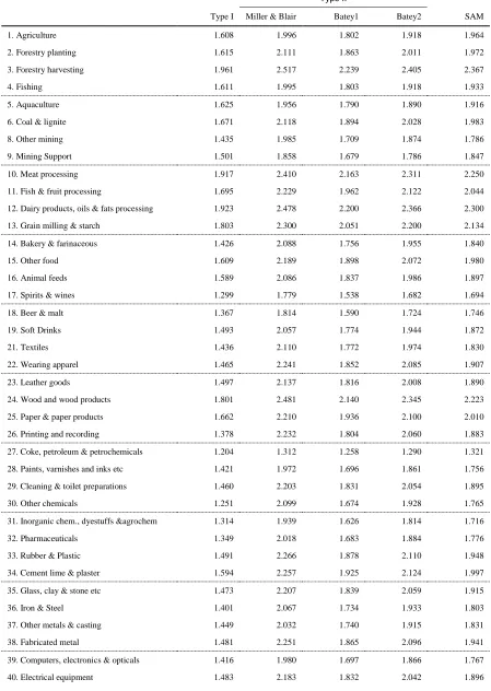
Table 1 compares the the IO Type I, Type II and SAM multiplier values across Scottish

industrial sectors for 2009. The Type II IO multipliers comprise the M+B, Batey1 and

Batey2 variants. The data used are the 2009 Scottish Industry by Industry (IxI) Table

(Scottish Government, 2013) and the 2009 Scottish SAM (Emonts-Holley et al., 2014).

The SAM is constructed around the corresponding IO accounts, so that the multiplier

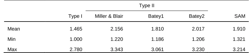
values are consistent. The deviations of the IO Type II multipliers for each sector from the

corresponding SAM multiplier value are given in Figure 1. The horizontal axis represent

the SAM multiplier value so that all the observations for each industry are measured

Table 1: IO and SAM multipliers for Scotland

Type II

Type I Miller & Blair Batey1 Batey2 SAM

1. Agriculture 1.608 1.996 1.802 1.918 1.964

2. Forestry planting 1.615 2.111 1.863 2.011 1.972

3. Forestry harvesting 1.961 2.517 2.239 2.405 2.367

4. Fishing 1.611 1.995 1.803 1.918 1.933

5. Aquaculture 1.625 1.956 1.790 1.890 1.916

6. Coal & lignite 1.671 2.118 1.894 2.028 1.983

8. Other mining 1.435 1.985 1.709 1.874 1.786

9. Mining Support 1.501 1.858 1.679 1.786 1.847

10. Meat processing 1.917 2.410 2.163 2.311 2.250

11. Fish & fruit processing 1.695 2.229 1.962 2.122 2.044

12. Dairy products, oils & fats processing 1.923 2.478 2.200 2.366 2.300

13. Grain milling & starch 1.803 2.300 2.051 2.200 2.134

14. Bakery & farinaceous 1.426 2.088 1.756 1.955 1.840

15. Other food 1.609 2.189 1.898 2.072 1.980

16. Animal feeds 1.589 2.086 1.837 1.986 1.897

17. Spirits & wines 1.299 1.779 1.538 1.682 1.694

18. Beer & malt 1.367 1.814 1.590 1.724 1.746

19. Soft Drinks 1.493 2.057 1.774 1.944 1.872

21. Textiles 1.436 2.110 1.772 1.974 1.830

22. Wearing apparel 1.465 2.241 1.852 2.085 1.907

23. Leather goods 1.497 2.137 1.816 2.008 1.890

24. Wood and wood products 1.801 2.481 2.140 2.345 2.223

25. Paper & paper products 1.662 2.210 1.936 2.100 2.010

26. Printing and recording 1.378 2.232 1.804 2.060 1.883

27. Coke, petroleum & petrochemicals 1.204 1.312 1.258 1.290 1.321

28. Paints, varnishes and inks etc 1.421 1.972 1.696 1.861 1.756

29. Cleaning & toilet preparations 1.460 2.203 1.831 2.054 1.895

30. Other chemicals 1.251 2.099 1.674 1.928 1.765

31. Inorganic chem., dyestuffs &agrochem 1.314 1.939 1.626 1.814 1.716

32. Pharmaceuticals 1.349 2.018 1.683 1.884 1.776

33. Rubber & Plastic 1.491 2.266 1.878 2.110 1.948

34. Cement lime & plaster 1.594 2.257 1.925 2.124 1.997

35. Glass, clay & stone etc 1.473 2.207 1.839 2.059 1.915

36. Iron & Steel 1.401 2.067 1.734 1.933 1.803

37. Other metals & casting 1.449 2.032 1.740 1.915 1.831

38. Fabricated metal 1.481 2.251 1.865 2.096 1.941

41. Machinery & equipment 1.519 2.304 1.911 2.146 1.983

42. Motor Vehicles 1.515 2.178 1.846 2.045 1.907

43. Other transport equipment 1.647 2.264 1.955 2.140 2.026

44. Furniture 1.574 2.284 1.928 2.141 1.999

45. Other manufacturing 1.403 2.301 1.851 2.121 1.913

46. Repair & maintenance 1.427 2.164 1.795 2.016 1.877

47. Electricity 2.053 2.405 2.229 2.335 2.345

48. Gas etc 1.260 1.544 1.401 1.487 1.482

49. Water and sewerage 1.287 1.733 1.509 1.643 1.708

50. Waste 1.493 2.195 1.843 2.054 1.941

51. Remediation & waste management 2.780 3.343 3.061 3.230 3.214

52. Construction – buildings 1.766 2.401 2.083 2.273 2.200

53. Construction - civil engineering 1.731 2.450 2.090 2.305 2.202

54. Construction – specialised 1.530 2.288 1.908 2.136 2.020

55. Wholesale & Retail – vehicles 1.335 2.116 1.725 1.959 1.815

56. Wholesale - excl vehicles 1.521 2.253 1.886 2.106 1.990

57. Retail - excl vehicles 1.352 2.139 1.745 1.981 1.858

58. Rail transport 1.764 2.582 2.172 2.418 2.265

59. Other land transport 1.400 2.033 1.716 1.906 1.810

60. Water transport 1.657 2.138 1.897 2.042 1.980

61. Air transport 1.467 1.920 1.693 1.829 1.792

62. Support services for transport 1.541 2.195 1.867 2.063 1.994

63. Post & courier 1.278 2.351 1.813 2.135 1.893

64. Accommodation 1.352 2.065 1.708 1.922 1.814

65. Food & beverage services 1.362 2.082 1.721 1.937 1.816

66. Publishing services 1.279 2.140 1.709 1.967 1.790

67. Film video & TV etc 1.454 2.100 1.777 1.970 1.869

68. Broadcasting 1.386 2.043 1.714 1.911 1.819

69. Telecommunications 1.393 2.067 1.729 1.931 1.859

70. Computer services 1.250 2.115 1.682 1.941 1.789

71. Information services 1.185 1.987 1.585 1.826 1.719

72. Financial services 1.222 1.785 1.503 1.671 1.665

73. Insurance & pensions 1.859 2.359 2.108 2.258 2.234

74. Auxiliary financial services 1.282 2.138 1.709 1.966 1.796

75. Real estate – own 1.465 1.768 1.616 1.707 1.817

76. Imputed rent 1.151 1.220 1.186 1.206 1.387

77. Real estate - fee or contract 1.503 2.198 1.850 2.059 1.971

78. Legal activities 1.241 2.069 1.655 1.903 1.781

79. Accounting & tax services 1.202 2.118 1.659 1.934 1.786

80. Head office & consulting services 1.391 2.267 1.828 2.091 1.914

81. Architectural services etc 1.437 2.239 1.838 2.078 1.953

85. Veterinary services 1.364 2.197 1.780 2.029 1.918

86. Rental and leasing services 1.324 1.911 1.617 1.793 1.751

87. Employment services 1.301 2.351 1.825 2.140 1.918

88. Travel & related services 1.520 1.936 1.728 1.852 1.786

89. Security & investigation 1.155 2.378 1.765 2.132 1.853

90. Building & landscape services 1.388 2.329 1.857 2.140 1.964

91. Business support services 1.285 1.985 1.634 1.844 1.769

92. Public administration & defence 1.410 2.240 1.824 2.073 1.903

93. Education 1.189 2.478 1.832 2.219 1.914

94. Health 1.362 2.290 1.825 2.103 1.902

95. Residential care 1.320 2.330 1.824 2.127 1.950

96. Social work 1.236 2.496 1.864 2.242 1.959

97. Creative services 1.474 2.398 1.935 2.212 2.005

98. Cultural services 1.356 2.382 1.868 2.176 1.948

99. Gambling 1.414 1.933 1.673 1.828 1.822

100. Sports & recreation 1.407 2.332 1.869 2.146 1.950

101. Membership organisations 1.436 2.329 1.882 2.150 1.970

102. Repairs - personal and household 1.357 2.121 1.738 1.967 1.822

103. Other personal services 1.233 1.947 1.590 1.804 1.732

104. Households as employers 1.000 2.405 1.701 2.122 1.799

Source: Author’s own calculations based on data in Scottish Government (2013) and

Emonts-Holley et al. (2014).

Table 1 and Figure 1 show that the ordering of the Type II IO multiplier values derived

from their analytical properties investigated in Section 6 are replicated in the data. For

every sector, M_iM B+ >M_iB2 >M_iB1and the SAM multiplier is always greater than the

Batey1 multiplier M_iB1>M_iS. There are two sectors, 75 and 76 - Real Estate and the

Imputed Rent - where the SAM multiplier has the highest value.3 In all other sectors

M B i

M + is the highest multiplier value. The Batey2 multiplier is generally above the SAM

value: in only 10 of the 104 sectors is it less. There are some very pronounced positive

spikes using the M+B and the Batey2 approach, where the value is large in comparison to

the SAM multiplier. The three most prominent examples are for sectors 89, 93 and 96,

which are Security & Investigation, Education, and Social Work respectively. These

results are driven by the relatively high share of labour in value added in these sectors.

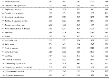
Table 2 gives the summary statistics for the range of multiplier values, showing the

maximum, minimum and mean figures. The first point to make is that if the mean values

for the Type I IO and SAM multipliers are compared, the incorporation of induced activity

increases the multiplier from 1.465 to 1.910. That is to say the additional output over and

above the direct increase in final demand is almost doubled by including the induced

household consumption effects. Second, as the evidence from Figure 1 suggests, the mean

value for the Batey1 Type II multiplier is lowest, followed by the SAM, the Batey2 and

finally the Miller and Blair values. The difference between the two extreme Type II mean

multiplier values is 0.346. The range of Type II multiplier values is almost 40% of the

most accurate measurement of additional multiplier effect, which is the SAM value 0.910.

Table 2: IO and SAM multiplier summart statistics

Type II

Type I Miller & Blair Batey1 Batey2 SAM Mean 1.465 2.156 1.810 2.017 1.910

Min 1.000 1.220 1.186 1.206 1.321

Max 2.780 3.343 3.061 3.230 3.214

Table 2 shows that the mean SAM multiplier lies within the range of the mean IO Type II

values. The Batey1 figure is systematically lower than the SAM multiplier and the Batey2

and M+B approaches systematically higher. Batey1 is the Type II IO multiplier whose

mean value is closest to the mean SAM multiplier, though this is only marginally closer

than Batey2. The minimum and maximum multiplier values also replicate these findings.

Table 3 calculates the Root Mean Square Error and Mean Absolute Error for the Type II

multiplier values for individual sectors against the SAM multiplier figure. Again the

Miller & Blair Batey1 Batey2 RMSE 0.201 0.077 0.099

Figure 1: Differences between the SAM and the Type II multipliers -0.3 -0.2 -0.1 0.0 0.1 0.2 0.3 0.4 0.5 0.6 0.7 1. A gr ic ul tu re 3. F or es tr y har v es ti ng 5. A quac ul tur e 8. O ther m ini ng 10. M eat pr oc es s ing ai ry pr oduc ts , oi ls & f at s pr oc e s s ing 14. B ak er y & f ar inac e ous 16. A ni m al f eeds 18. B eer & m al t 21. T ex ti les 23. Lea ther goods 25. P aper & paper pr oduc ts C ok e, pet rol eum & pet roc he m ic al s 29. C leani ng & t o ilet pr epar at io ns 31. I nor gani c c h em ic al s , dy es tuf fs 33. R ub ber & P las ti c 35. G las s , c lay & s tone et c 37. O ther m et al s & c as ti ng C om put er s , e lec tr o ni c s & opt ic a ls 41. M ac hi ner y & eq ui pm ent 43. O ther t ran s por t equ ipm ent 45. O ther m anuf ac tur ing 47. E lec tr ic it y 49. Wat er and s ew er age R em edi at ion & w as te m an agem ent 53. C on s tr uc ti on c iv il e ngi n eer ing 55. Whol es al e & R et ai l - v ehi c les 57. R et ai l ex c l v eh ic le s 59. O ther l an d t rans p or t 61. A ir t rans por t 63. P os t & c our ier 65. F ood & bev er age s er v ic e s 67. F ilm v ideo & T V et c 69. T el ec om m u ni c at ions 71. I nf o rm at ion s er v ic e s 73. I ns ur anc e & pens ions 75. R ea l es tat e ow n 77. R ea l es tat e f ee or c ont rac t 79. A c c ou nt ing & t ax s er v ic es 81. A rc hi tec tur al s er v ic e s et c 83. A dv er ti s ing & m ar k et r es ear c h 85. V et er in ar y s er v ic es 87. E m pl oy m ent s er v ic e s 89. S ec ur it y & i n v es ti gat ion 91. B us ines s s uppor t s er v ic es 93. E duc at ion 95. R es ident ial c ar e 97. C reat iv e s er v ic es 99. G am bl in g 101. M em ber s hi p or gani s at ions 103. O ther per s on al s er v ic es

Miller & Blair

Batey1

8. Discussion and conclusion

There is complete agreement about the method used to calculate Input-Output Type I

multipliers. These measure the direct and indirect output effects from a unit expansion in

exogenous final demand in a particular sector. They incorporate the change in activity

associated with the production of the intermediate goods that contribute directly or

indirectly to the production of final demand.

Type II multipliers identify the direct and indirect effects. However, they also incorporate

the impact of increased household income and subsequent consumption expenditure that

accompanies any change in output. These are known as induced effects. Although this is a

very common procedure, a number of different methods have been adopted in the

literature. First, we believe that this variation is not widely recognised. This is potentially

problematic for the interpretation of Type II multipliers, their use in modelling

demand-side disturbances and the value for comparing the structural characteristics of different

economies. Second, it would be valuable to standardise the Type II procedure, which

requires choosing amongst the different formulations.

The first question is whether empirically this is a serious problem. The Scottish results

suggest that it is. The range of Type II multiplier mean values is almost 40% of the most

accurate measurement of additional multiplier effect. The second question is: which

method is preferable? If the SAM multipliers embody the most complete linking of

income generated in production and the subsequent distribution to households.for

Scotland the mean value using the Batey1 method is closest to the mean SAM value and

has the smallest mean error, even though the method systematically underestimates the

SAM multiplier values. However, this method has the disadvantage that it requires

information on household income that is typically not available from the IO accounts

themselves.

Despite some of the models coming close to SAM multipliers, it must be acknowledged

wages, and link household expenditure to these. A SAM multiplier incorporates income

from other value added into household income in a way completely consistent with the

standard demand-driven IO approach. It is therefore the only wholly satisfactory means of

Appendix 1: Variable names and symbols

Symbol Variable name

A Matrix of technical coefficients in production

B Matrix of Type II coefficients

C Total household consumption

M Multiplier value

N Endogenous (subscript)

R Total corporate income

S Matrix of SAM coefficients

T Exogenous transfers

W Total wages

X Exogenous (subscript)

Z Identifier for Type II multiplier

c Household consumption vector

f Vector of final demands

rK Share of corporate income distributed to account K

v Vector of institutional income

w Vector of production wage coefficients

x Vector of output

Π Total other value added

ij

α Elements of the Type I Leontief inverse

ij

β Elements of the Type II Leontief inverse

i

ϕ Coefficients of household consumption expenditure

ij

κ Income adjustment in the modified Type II matrix of coefficients

K

ρ Share of other value added income distributed to account K

References

Batey, P. (1985), “Input-output Models for Regional Demographic-Economic Analysis:

Some Structural Comparisons”, Environment and Planning A, vol. 17, pp. 73-99.

Batey, P. and Madden, M. (1983), “Linked Population and Economic Models: Some

Methodological Issues in Forecasting, Analysis and Policy Optimisation”, Journal of

Regional Science, vol. 23, pp. 141-164.

Batey, P. and Weeks, M.J. (1989), “The Effects of Household Disaggregation in Extended

Input-Output Models”, in R.E. Miller, K.R. Polenske and A.Rose, eds., Frontiers of

Input-Output Analysis: Commemorative Papers, Oxford University Press, New York.

Emonts-Holley, T., Ross, A., & Swales, J.K. (2014), “A Social Accounting Matrix for

Scotland”, Fraser of Allander Institute Economic Commentary, 38(1), 84-93.

Miller, R., & Blair, P. (1985), Input-Output Analysis Foundations and Extensions,

Prince-Hall.

Round, J. (2003), Social Accounting Matrices and SAM-based Multiplier Analysis.

Chapter 14 in F. Bourguignon and L.A. Pereira da Silva eds., Techniques and Tools for

Evaluating the Poverty Impact of Economic Policies, World Bank and Oxford University

Press.