Adjusting treatment effect estimates by post-stratification in randomized experiments

Adjusting treatment effect

estimates by post-stratification

in randomized experiments

The Harvard community has made this

article openly available. Please share how

this access benefits you. Your story matters

Citation

Miratrix, Luke W., Jasjeet S. Sekhon, and Bin Yu. 2012. “Adjusting

Treatment Effect Estimates by Post-Stratification in Randomized

Experiments.” Journal of the Royal Statistical Society: Series B

(Statistical Methodology) 75 (2) (December 4): 369–396. doi:10.1111/

j.1467-9868.2012.01048.x.

Published Version

doi:10.1111/j.1467-9868.2012.01048.x

Citable link

http://nrs.harvard.edu/urn-3:HUL.InstRepos:30501585

Adjusting Treatment Effect Estimates by Post-Stratification in

Randomized Experiments

Luke W. Miratrix† Jasjeet S. Sekhon‡ Bin Yu§

Forthcoming,Journal of the Royal Statistical Society, Series B (Methodology)

August 10, 2012 (16:26)

Abstract

Experimenters often use post-stratification to adjust estimates. Post-stratification is akin to blocking, except that the number of treated units in each stratum is a random variable be-cause stratification occurs after treatment assignment. We analyze both post-stratification and blocking under the Neyman-Rubin model and compare the efficiency of these designs. We derive the variances for a post-stratified estimator and a simple difference-in-means estimator under different randomization schemes. Post-stratification is nearly as efficient as blocking: the difference in their variances is on the order of1/n2_{, with a constant depending on}

treat-ment proportion. Post-stratification is therefore a reasonable alternative to blocking when the latter is not feasible. However, in finite samples, post-stratification can increase variance if the number of strata is large and the strata are poorly chosen. To examine why the estimators’ vari-ances are different, we extend our results by conditioning on the observed number of treated units in each stratum. Conditioning also provides more accurate variance estimates because it takes into account how close (or far) a realized random sample is from a comparable blocked experiment. We then show that the practical substance of our results remain under an infinite population sampling model. Finally, we provide an analysis of an actual experiment to illustrate our analytical results.

Keywords: Neyman-Rubin model; blocking; regression adjustment; randomized trials

∗

We thank Peter Aronow, Winston Lin, Terry Speed, and Jonathan Wand for helpful comments. Luke Miratrix is grateful for the support of a Graduate Research Fellowship from the National Science Foundation. This work is supported in part by NSF grant SES-0835531 (CDI). The authors are responsible for all errors.

†

Assistant Professor, Department of Statistics, Harvard University. Email: [email protected]. Mail: Science Center, 1 Oxford Street, Cambridge, MA 02138-2901

‡

Professor, Travers Department of Political Science, Department of Statistics, and Director, Center for Causal In-ference and Program Evaluation, Institute of Governmental Studies, UC Berkeley, Berkeley, CA 94720. http: //sekhon.berkeley.edu

§

1

Introduction

One of the most important tools for determining the causal effect of some action is the randomized experiment, where a researcher randomly divides units into groups and applies different treatments to each group. Randomized experiments are the “gold standard” for causal inference because, as-suming proper implementation of the experiment, if a difference in outcomes is found, the only possible explanations are a significant treatment effect or random chance. Analytical calculation gives a handle on the chance which allows for principled inference about the treatment effect. In the most basic analysis, a simple difference in means is used to estimate the overall sample average treatment effect (SATE), defined as the difference in the units’ average outcome if all were treated as compared to their average outcome if they were not. This framework and estimator were analyzed by Neyman in 19231 under what is now called the Neyman or Neyman-Rubin model of potential outcomes (Holland, 1986). Under this model, one need make few assumptions not guaranteed by the randomization itself.

Since each additional observation in an experiment sometimes comes at considerable cost, it is desirable to find more efficient estimators than the simple difference-in-means estimator to measure treatment effects. Blocking, which is when experimenters first stratify their units and then ran-domize treatment within pre-defined blocks, can greatly reduce variance compared to the simple-difference estimator if the strata differ from each other. See “A Useful Method” in Fisher (1926) for an early overview, Wilk (1955) for an analysis and comparison with ANOVA, or Imai et al. (2008) for a modern overview. Unfortunately, because blocking must be conducted before ran-domization, it is often not feasible due to practical considerations or lack of foresight. Sometimes randomization may even be entirely out of the researcher’s control, such as with so-called natural experiments. When blocking is not done, researchers often adjust for covariates after randomiza-tion. For example, Pocock et al. (2002) studied a sample of clinical trials analyses and found that 72% of these articles used covariate adjustment. Keele et al. (2009) analyzed the experimental re-sults in three major political science journals and found that 74% to 95% of the articles relied on adjustment. Post-stratification is one simple form of adjustment where the researcher stratifies ex-perimental units with a pretreatment variable, estimates treatment effects within the strata, and then uses a weighted average of these strata estimates for the overall average treatment effect estimate. This is the estimator we focus on.

In this paper, we use the Neyman-Rubin model to compare post-stratification both to block-ing and to usblock-ing no adjustment. Neyman’s framework does not require assumptions of a constant treatment effect or of identically or independently distributed disturbances, assumptions typically made when considering adjustment to experimental data without this framework (e.g., McHugh and Matts, 1983). This avenue for a robust analysis, revitalized by Rubin in the 1970s (Rubin, 1974), has recently had much appeal. See, for example, work on general experiments (Keele et al., 2009), matched pairs (Imai, 2008), or matched pairs of clusters (Imai et al., 2009).2 Also see Neyman’s own treatment of blocking in the appendix of Neyman et al. (1935). Our estimator is equivalent to one from a fully saturated OLS regression. Freedman (2008a,b) analyzed the regression-adjusted estimator under the Neyman-Rubin model without treatment-by-strata interactions and found that the asymptotic variance might be larger than if no correction were made. Lin (2012) extended Freedman’s results and showed that when a treatment-by-covariate interaction is included in the regression, adjustment cannot increase the asymptotic variance. We analyze the exact, finite sample properties of this saturated estimator. Imbens (2011) analyzed estimating the treatment effect in

1_{See the English translation by Splawa-Neyman et al. (1990).}

a larger population, assuming the given sample being experimented on is a random draw from it. However, because in most randomized trials the sample is not taken at random from the larger popu-lation of interest, we focus on estimating the treatment effect within the sample. Tsiatis et al. (2008) and Koch et al. (1998) proposed other adjustment methods that also rely on weak assumptions and that have the advantage of working naturally with continuous or multiple covariates. Due to differ-ent sets of assumptions and methods of analysis, these estimators have important differences from each other. See Section 6 for further discussion.

We derive the variances for post-stratification and simple difference-in-means estimators un-der many possible randomization schemes including complete randomization and Bernoulli assign-ment. We show that the difference between the variance of the post-stratified estimator and that of a blocked experiment is on the order of1/n2with a constant primarily dependent on the proportion of units treated. Post-stratification is comparable to blocking. Like blocking, post-stratification can greatly reduce variance over using a simple difference-in-means estimate. However, in small sam-ples post-stratification can substantially hurt precision, especially if the number of strata is large and the stratification variable poorly chosen.

After randomization, researchers can observe the proportion of units actually treated in each stratum. We extend our results by deriving variance formula for the post-stratified and simple-difference estimators conditioned on these observed proportions. These conditional formula help explain why the variances of the estimators can differ markedly with a prognostic covariate: the difference comes from the potential for bias in the simple-difference estimator when there is large imbalance (i.e., when the observed proportions of units treated are far from what is expected). In-terestingly, if the stratification variable is not predictive of outcomes the conditional MSE of the simple-difference estimator usually remains the same or even goes down with greater imbalance, while the conditional MSE of the adjusted estimator increases. Adjusting for a poorly chosen co-variate has real cost in finite samples.

The rest of the paper is organized as follows: In the next section, we set up the Neyman-Rubin model, describe the estimators, and then derive the estimators’ variances. In Section 3 we show that post-stratification and blocking have similar characteristics in many circumstances. In Section 4, we present our formula for the estimators’ variances conditioned on the observed proportions of treated units in the strata and discuss their implications. We then align our results with those of Imbens (2011) in Section 5 by extending our findings to the super-population model and discussing the similarities and differences of the two viewpoints. We compare post-stratification to other forms of adjustment in Section 6, focusing on how these different approaches use different assumptions. In Section 7, we apply our method to the real data example of a large, randomized medical trial to assess post-stratification’s efficacy in a real-world example. We also make a hypothetical example from this data set to illustrate how an imbalanced randomization outcome can induce bias which the post-stratified estimator can adjust for. Section 8 concludes.

2

The Estimators and Their Variances

We consider the Neyman-Rubin model with two treatments andnunits. For an example consider a randomized clinical trial withnpeople, half given a drug and the other half given a placebo. Let

yi(1)∈Rbe uniti’s outcome if it were treated, andyi(0)its outcome if it were not. These are the

potential outcomesof uniti. For each unit, we observe eitheryi(1)oryi(0)depending on whether

patient would have no impact on the outcome of any other patient. The treatment effecttifor uniti

is then the difference in potential outcomes,ti ≡yi(1)−yi(0), which is deterministic.

Although theseti are the quantities of interest, we cannot in general estimate them because we

cannot observe both potential outcomes of any unitiand because thetigenerally differ by unit. The

average across a population of units, however, is estimable. Neyman (Splawa-Neyman et al., 1990) considered the overall Sample Average Treatment Effect, or SATE:

τ ≡ 1

n

n X

i=1

[yi(1)−yi(0)]

To conduct an experiment, randomize units into treatment and observe outcomes. Many choices of randomization are possible. The observed outcome is going to be one of the two potential outcomes, and which one depends on the treatment given. Random assignment gives a treatment assignment vectorT = (T1, . . . , Tn)withTi ∈ {0,1}being an indicator variable of whether unitiwas treated

or not. T’s distribution depends on how the randomization was conducted. After the experiment is complete, we obtain the observed outcomesY, withYi =Tiyi(1) + (1−Ti)yi(0). The observed

outcomes are random—but only due to the randomization used. The yi(`) andti are all fixed.

Neyman first considered abalanced complete randomization:

Definition 2.1 (Complete Randomization of n Units). Given a fixed p ∈ (0,1) such that 0 < pn < nis an integer, aComplete Randomizationis a simple random sample ofpnunits selected for treatment with the remainder left as controls. If p = 0.5(andnis even) the randomization is

balancedin that there are the same number of treated units as control units.

The classic unadjusted estimatorτˆsdis the observedsimple differencein the means of the

treat-ment and control groups:

ˆ τsd =

1 W(1)

n X

i=1

TiYi−

1 W(0)

n X

i=1

(1−Ti)Yi

=

n X

i=1

Ti

W(1)yi(1)−

n X

i=1

(1−Ti)

W(0) yi(0),

where W(1) = P

iTi is the total number of treated units, W(0) is total control, and W(1) +

W(0) = n. For Neyman’s balanced complete randomization, W(1) = W(0) = n/2. For other randomizations schemes theW(`)are potentially random.

We analyze the properties of various estimators based on the randomization scheme used— this is the source of randomness. Fisher proposed a similar strategy for testing the “sharp null” hypothesis of no effect (whereyi(0) = yi(1)fori= 1, . . . , n); under this view, all outcomes are

known and the observed difference in means is compared to its exact, known distribution under this sharp null. Neyman, in contrast,estimatedthe variance of the difference in means, allowing for the unknown counterfactual outcomes of the units to vary. These different approaches have different strengths and weaknesses that we do not here discuss. We follow this second approach.

Neyman showed that the variance ofτˆsdis

Var[ˆτsd] =

2 nE

s2₁+s2₀

− 1 nS

2 ₍₁₎

where s2_` are the sample variances of the observed outcomes for each group, S2 is the variance of then treatment effectsti, and the expectation is over all possible assignments under balanced

2.1 The Post-Stratified Estimator of SATE

Stratification is when an experimenter divides the experimental units into K strata according to some categorical covariateb withbi ∈ B ≡ {1, . . . , K}, i = 1, . . . , n. Each stratumkcontains

nk = #{i : bi = k} units. For example, in a cancer drug trial we might have the strata being

different stages of cancer. If the strata are associated with outcome, an experimenter can adjust a treatment effect estimate to remove the impact of random variability in the proportions of units treated. This is the idea behind post-stratification. The bi are observed for all units and are not

affected by treatment. The strata defined by the levels ofbhave stratum-specific SATEk:

τk≡

1 nk

X

i:bi=k

[yi(1)−yi(0)] k= 1, . . . , K.

The overall SATE can then be expressed as a weighted average of these SATEks:

τ = X

k∈B

nk

nτk. (2)

We can view the strata as K mini-experiments. Let Wk(1) = P

i:bi=kTi be the number of treated units in stratumk, andWk(0)be the number of control units. We can use a simple-difference

estimator for each stratum to estimate the SATEks:

ˆ τk =

X

i:bi=k

Ti

Wk(1)

yi(1)− X

i:bi=k

(1−Ti)

Wk(0)

yi(0), (3)

A post-stratification estimator is an appropriately weighted estimate of these strata-level estimates:

ˆ τps ≡

X

k∈B

nk

n ˆτk. (4)

These weights echo the weighted sum of SATEks in Equation 2. Becausebandnare known and

fixed, the weights are also known and fixed. We derive the variance ofˆτpsin this paper.

Technically, this estimator is undefined if Wk(1) = 0 orWk(0) = 0 for anyk ∈ 1, . . . , K.

We therefore calculate all means and variances conditioned on D, the event that τˆps is defined,

i.e., that each stratum has at least one unit assigned to treatment and one to control. This is fairly natural: if the number of units in each stratum is not too small the probability ofD is close to 1 and the conditioned estimator is similar to an appropriately defined unconditioned estimator. See Section 2.2. Similarly,τsdis undefined ifW(1) = 0orW(0) = 0. We handle this similarly, letting

D0be the set of randomizations whereτˆsdis defined.

Different experimental designs and randomizations give different distributions on the treatment assignment vectorT and all resulting estimators. Some distributions on T would cause bias. We disallow those. Define theTreatment Assignment Patternfor stratumkas the ordered vector(Ti :

i∈ {1, . . . , n:bi=k}). We assume that the randomization used hasAssignment Symmetry:

Definition 2.2(Assignment Symmetry). A randomization isAssignment Symmetricif the following two properties hold:

1. Equiprobable Treatment Assignment Patterns

All nk

Wk(1)

ways to treatWk(1)units in stratumkare equiprobable, givenWk(1).

2. Independent Treatment Assignment Patterns

Complete randomization and Bernoulli assignment (where independent p-coin flips determine treatment for each unit) satisfy Assignment Symmetry. So does blocking, where strata are random-ized independently. Furthermore, given a distribution on T that satisfies Assignment Symmetry, conditioning on Dmaintains Assignment Symmetry (as do many other reasonable conditionings, such as having at leastxunits in both treatment and control). See the supplementary material for a more formal argument. Cluster randomization or randomization where units have unequal treatment probabilities do not, in general, have Assignment Symmetry. In our technical results, we assume that (1) the randomization is Assignment Symmetric and (2) we are conditioning onD, the set of possible assignments whereτˆpsis defined.

The post-stratification estimator and the simple-difference estimator are used when the initial random assignment ignores the stratification variableb. In a blocked experiment, the estimator used isτˆps, but the randomization is done within the strata defined byb. All three of these options are

unbiased. We are interested in their relative variances. We express the variances of these estimators with respect to the sample’s (unknown) means, variances and covariance of potential outcomes divided into between-strata variation and within-stratum variation. The within-stratum variances and covariances are, fork= 1, . . . , K:

σ_k2(`) = 1 nk−1

X

i:bi=k

[yi(`)−y¯k(`)]2 `= 0,1

and

γk(1,0) =

1 nk−1

X

i:bi=k

[yi(1)−y¯k(1)] [yi(0)−y¯k(0)],

wherey¯k(`)denotes the mean ofyi(`)for all units in stratumk. Like many authors, we usenk−1

rather thannkfor convenience and cleaner formula. The(1,0)inγk(1,0)indicates that this

frame-work could be extended to multiple treatments.

The between-stratum variances and covariance are the weighted variances and covariance of the strata means:

¯

σ2(`) = 1 n−1

K X

k=1

nk[¯yk(`)−y(`)]¯ 2 `= 0,1

and

¯

γ(1,0) = 1 n−1

K X

k=1

nk[¯yk(1)−y(1)] [¯¯ yk(0)−y(0)]¯ .

The population-wide σ2(`) and γ(1,0)are analogously defined. They can also be expressed as weighted sums of the component pieces. We also refer to thecorrelation of potential outcomesr, wherer≡γ(1,0)/σ(0)σ(1)and thestrata-level correlationsrk, whererk≡γk(1,0)/σk(0)σk(1).

An overall constant treatment effect givesr = 1,σ(0) =σ(1),rk= 1for allkandσk(0) =σk(1)

for allk.

We are ready to state our main results:

Theorem 2.1. The strata-level estimatorsτˆkare unbiased, i.e.

E[ˆτk|D] =τk k= 1, . . . , K

and their variances are

Var[ˆτk|D] =

1 nk

β1kσk2(1) +β0kσ2k(0) + 2γk(1,0)

withβ1k=E[Wk(0)/Wk(1)|D], the expected ratio of the number of units in control to the number

of units treated in stratumk, andβ0k=E[Wk(1)/Wk(0)|D], the reverse. Theorem 2.2. The post-stratification estimatorτˆpsis unbiased:

E[ˆτps|D] =E

"

X

k

nk

nτˆk|D

#

=X

k

nk

n E[ˆτk|D] =

X

k

nk

n τk=τ.

Its variance is

Var[ˆτps|D] =

1 n

X

k

nk

n

β1kσ2k(1) +β0kσk2(0) + 2γk(1,0)

. (6)

See Appendix A for a proof. In essence we expand the sums, use iterated expectation, and eval-uate the means and variances of the treatment indicator random variables. Assignment Symmetry allows for the final sum. Techniques used are similar to those found in many papers classic (e.g., Neyman et al. (1935); Student (1923)) and recent (e.g., Imai et al. (2008)).

Consider the whole sample as a single stratum and use Theorem 2.1 to immediately get:

Corollary 2.3. The unadjusted simple-difference estimatorτˆsd is unbiased, i.e. E[ˆτsd|D0] =τ. Its

variance is

Varτˆsd|D0

= 1

n

β1σ2(1) +β0σ2(0) + 2γ(1,0)

, (7)

whereβ1≡E[W(0)/W(1)|D0]andβ0 ≡E[W(1)/W(0)|D0]. In terms of strata-level parameters,

its variance is

Varτˆsd|D0

= 1

n

β1¯σ2(1) +β0σ¯2(0) + 2¯γ(1,0)

+

1 n

X

k

nk−1

n−1

β1σk2(1) +β0σ2k(0) + 2γk(1,0)

. (8)

Conditioning τˆsd on the D associated withτˆps does not produce an Assignment Symmetric

randomization in the single stratum of all units, and indeedE[ˆτsd|D]6=τ in some cases.

For completely randomized experiments with np units treated, β1 = (1−p)/p and β0 =

p/(1−p). For a balanced completely randomized experiment, Equation 7 is the result presented in Splawa-Neyman et al. (1990)—see Equation 1; the expectation of the sample variance is the overall variance. Thenβ` = 1and

Var[ˆτsd] =

1 n σ

2_{(1) +σ}2_{(0) + 2γ(1,0)}

= 2 n σ

2_{(1) +σ}2₍₀₎

− 1 n σ

2_{(1) +σ}2_{(0)−2γ(1,0)}

= 2 n σ

2_{(1) +σ}2₍₀₎

− 1

nVar[yi(1)−yi(0)].

Remarks. β1k is the expectation ofWk(0)/Wk(1), the ratio of control units to treated units in

stratumk. For largenk, this ratio is close to the ratioE[Wk(0)]/E[Wk(1)]since theWk(`)will not

vary much relative to their size. For smallnk, however, they will vary more, which tends to result in

post-stratification differs from blocking. This is discussed more formally later on and in Appendix B.

For `= 0,1theβ`k’s are usually larger thanβ`, being expectations of different variables with

different distributions. For example in a balanced completely randomized experimentβ1 = 1but

β1k>1fork= 1, . . . , KsinceWk(1)is random andW(1)is not.

All the β’s depend on both the randomization and the conditioning on DorD0, and thus the variances from both Equation 8 and Equation 6 can change (markedly) under different randomiza-tion scenarios. As a simple illustrarandomiza-tion, consider a complete randomizarandomiza-tion of a 40 unit sample with a constant treatment effect and four strata of equal size. Let allσk(`) = 1and allrk = 1. Also let

¯

σ(`) = ¯γ(0,1) = 0.56. Ifp = 0.5, thenβ1 = β0 = 1 and the variance ofˆτsd is about 0.15. If

p= 2/3thenβ1 = 1/2andβ0 = 2. Equation 8 holds in both cases, but the variance in the second

case will be about10%larger due to the largerβ0. There are fewer control units, so the estimate

of the control outcome is more uncertain. The gain in certainty for the treatment units does not compensate enough. Forp= 0.5,β1k=β0k≈1.21. The post-stratified variance is about0.11. For

p= 2/3,β1k≈2.44andβ0k ≈0.61. The average is about1.52. The variance is about14%larger

than thep = 0.5case. Generally speaking, the relative variances of different experimental setups are represented in theβ’s.

The correlation of potential outcomes, γk(1,0), can radically impact the variance. If they are

maximally negative, the variance can be zero or nearly zero. If they are maximally positive (as in the case of a constant treatment effect), the variance can be twice what it would be if the outcomes were uncorrelated.

Comparing the Estimators. Bothτˆps andτˆsd are unbiased, so their MSEs are the same as their

variances. To compareτˆpsandτˆsdtake the difference of their variances:

Varτˆsd|D0

−Var[ˆτps|D] =

1 n β1σ¯

2_{(1) +β}

0σ¯2(0) + 2¯γ(1,0)

−

(

1 n

K X

k=1

nk

nβ1k−

nk−1

n−1 β1

σ_k2(1) +

nk

n β0k−

nk−1

n−1 β0

σ_k2(0)

+

2 n2

K X

k=1

n−nk

n−1 γk(1,0)

)

. (9)

Equation 9 breaks down into two parts as indicated by the curly brackets. The first part,

β1σ¯2(1) +β0σ¯2(0) + 2¯γ(1,0), is the between-strata variation. It measures how much the mean

potential outcomes vary across strata and captures how well the stratification variable separates out different units, on average. The larger the separation, the more to gain by post-stratification. The second part, consisting of the bottom two lines of Equation 9, represents the cost paid by post-stratification due to, primarily, the chance of random imbalance in treatment causing units to be weighted differently. This second part is non-positive and is a penalty except in some cases where the proportion of units treated is extremely close to 0 or 1 or is radically different across strata.

To assess the magnitude of the penalty paid compared to the gain, multiply Equation 9 byn. The first term, representing the between-strata variation, is now a constant, and the scaled gain converges to it asngrows:

Theorem 2.4. Take an experiment withnunits randomized under either complete randomization or Bernoulli assignment. Letpbe the expected proportion of units treated. Without loss of generality, assume0.5≤p <1. Letf = min{nk/n:k= 1, . . . , K}be the proportional size of the smallest

stratum. Letσ2

max = maxk,`σ2k(`)be the largest variance of all the strata. Similarly defineγmax.

Then the scaled cost term is bounded:

n Var

ˆ τsd|D0

−Varτˆps|D0

−β1σ¯2(1)−β0σ¯2(0)−2¯γ(1,0)

≤C

1 n+O(

1 n2)

with

C =

8 f(1−p)2+

2p 1−p

σ_max2 + 2Kγmax.

See Appendix B for the derivation. Theorem 2.4 shows us that the second part of Equation 9, the harm, diminishes quickly.

ConditioningτˆpsonDandτˆsdonD0is not ideal, butˆτsdconditioned onDcan be biased if the

strata are unequal sizes andp 6= 0.5. However, due to a similar argument to that in Section 2.2, this bias is small and Equation 8 is close (i.e., within an exponentially small amount) to the MSE ofτˆsd conditioned onD. Thus Theorem 2.4 holds for both estimators conditioned onD. Indeed,

Theorem 2.4 holds unconditionally if the estimators extended so they are reasonably defined (e.g. set to 0) when¬Doccurs.

If the number of strata K grows withn, as is often the case when coarsening a continuous covariate, the story can change. The second and third lines of Equation 9 are sums overKelements. The larger the number of strataK, the more terms in the sums and the greater the potential penalty for stratification, unless theσ2_k(`)’s shrink in proportion asK grows. For an unrelated covariate, they will not tend to do so. To illustrate, we made a sequence of experiments increasing in size with a continuous covariatezunrelated to outcome. For each experiment withnunits, we constructedb

by cuttingzintoK =n/10chunks. Post-stratification was about 15% worse, in this case, than the simple-difference estimator regardless ofn. See our supplementary materials for details as well as other illustrative examples. Theorem 2.4 captures the dependence on the number of strata through

f, the proportional size of the smallest strata. If f ∝ 1/K then the difference will beO(K/n). For example, if K grows at rate O(logn), then the scaled difference will be O(logn/n), nearly

O(1/n).

Overall, post-stratifying on variables not heavily related to outcome is unlikely to be worthwhile and can be harmful. Post-stratifying on variables that do relate to outcome will likely result in large between-strata variation and thus a large reduction in variance as compared to a simple-difference estimator. More strata are not necessarily better, however. Simulations suggest that there is often a law of diminishing returns. For example, we made a simulated experiment withn = 200units with a continuous covariatezrelated to outcome. We then madebby cuttingzup intoK chunks forK = 1, . . . ,20. AsKincreased from 1 there was a sharp drop in variance and then, as the cost due to post-stratification increased, the variance leveled off and then climbed. In this case,K = 5

was ideal. We did a similar simulation for a covariatezunrelated to outcome. Now, regardless of

K, theσ2

k(`) were all about the same and the between-strata variation fairly low. AsK grew, the

overall variance climbed. In many cases a few moderate-sized strata give a dramatic reduction in variance, but having more strata beyond that has little impact, and can even lead to an increase in

ˆ

Estimation. Equation 6 and Equation 8 are the actual variances of the estimators. In practice, the variance of an estimator, i.e., the squared standard error, would have to itself be estimated. Unfortunately, however, it is usually not possible to consistently estimate the standard errors of difference-in-means estimators due to so-called identifiability issues as these standard errors de-pend on rk, the typically un-estimable correlations of the potential outcomes of the units being

experimented on (see Splawa-Neyman et al. (1990)). One approach to consistently estimate these standard errors is to impose structure to render this correlation estimable or known; Reichardt and Gollob (1999), for example, demonstrated that quite strong assumptions have to be made to obtain an unbiased estimator for the variance ofτˆsd. It is straightforward, however, to make a conservative

estimate by assuming the correlation is maximal. Sometimes there can be nice tricks—Alberto and IMBENS (2008), for example, estimated these parameters for matched-pairs by looking at pairs of pairs matched on covariates—but generally bounding the standard error is the best one can do. It is quite possible that for small samples the increased uncertainty and degrees-of-freedom issues in estimating the many variances composing the standard error of the post-stratification estimator cou-pled with this need to conservatively bound the correlation of potential outcomes could overwhelm any potential gains. Teasing this out is an area for future work.

That being said, all terms except theγk(1,0)in Equation 9 are estimable with standard sample

variance, covariance, and mean formula. In particular,γ¯(1,0)is estimable. By then making the conservative assumption that the γk(1,0)are maximal (i.e., thatrk = 1 for all k soγk(1,0) =

σ(1)σ(0)), we can estimate a lower-bound on the gain. Furthermore, by then dividing by a similar upper bound on the standard error of the simple-difference estimator, we can give a lower-bound on the percentage reduction in variance due to post-stratification. We illustrate this when we analyze an experiment in Section 7.

2.2 Not Conditioning onDChanges Little

Our results are conditioned onD, the set of assignments such thatWk(`) 6= 0for allk = 1, . . . K

and`= 0,1. This, it turns out, results in variances only slightly different from not conditioning on

D.

Setτˆps = 0if¬Doccurs, i.e. ifWk(`) = 0for somek, `. Other choices of how to define the

estimator when¬Doccurs are possible, including lettingτˆps = ˆτsd—the point is that this choice

does not much matter. In our caseE[ˆτps] =τPD. The estimate of the treatment is shrunk byPD

towards 0. It is biased byτP¬D. The variance is

Var[ˆτps] =Var[ˆτps|D]PD+τ2P¬DPD

and the MSE is

M SE[ˆτps] =E(ˆτps−τ)2

=Var[ˆτps|D]PD+τ2P¬D.

Not conditioning onDintroduces a bias term and some extra variance terms. All these terms are small ifP¬Dis near 0, which it is: P¬DisO(ne−n)(see Appendix B). Not conditioning onD, then, gives substantively the same conclusions as conditioning onD, but the formulae are a bit more unwieldy. Conditioning on the set of randomizations whereτˆpsis defined is more natural.

The above of course applies toτˆsd andD0 as well—and with a faster rate of decay since the

single stratum is the entire sample. Furthermore, this also means conditioning on the “wrong”D

is also negligible; i.e., ˆτsd conditioned onD is effectively unbiased. So the difference between

3

Comparing Blocking to Post-Stratification

Let theassignment splitW of a random assignment be the number of treated units in the strata:

W ≡(W1(1), . . . , WK(1))

Arandomized block trial ensures thatW is constant because we randomize within strata, en-suring a pre-specified number of units are treated in each. This randomization is Assignment Sym-metric (Def 2.2) and under it the probability of being defined,D, is 1. For blocking, the standard estimate of the treatment effect has the same expression asτˆps, but the Wk(`)s are all fixed. If all

blocks have the same proportion treated (i.e.,Wk(1)/nk =W(1)/nfor allk),τˆpscoincides with

ˆ τsd.

BecauseW is constant

β1k =E

Wk(0)

Wk(1)

= Wk(0) Wk(1)

= 1−pk pk

, (10)

wherepkis the proportion of units assigned to treatment in stratumk. Similarly,β0k=pk/(1−pk).

Letting the subscript “blk” denote this randomization, plug Equation 10 into Equation 6 to get the variance of a blocked experiment:

Varblk[ˆτps] =

1 n

X

k

nk

n

1−pk

pk

σ_k2(1) + pk 1−pk

σ_k2(0) + 2γk(1,0)

. (11)

Post-stratification is similar to blocking, and the post-stratified estimator’s variance tends to be close to that of a blocked experiment. Taking the difference between Equation 6 and Equation 11 gives

Var[ˆτps|D]−Varblk[ˆτps] =

1 n

X

k

nk

n

β1k−

1−pk

pk

σ_k2(1) +

β0k−

pk

1−pk

σ_k2(0)

. (12)

Theγk(1,0)cancelled; Equation 12 is identifiable and therefore estimable.

Randomization without regard tobcan have block imbalance due to ill luck:W is random. The resulting cost in variance of post-stratification over blocking is represented by theβ1k−(1−pk)/pk

terms in Equation 12. This cost is small, as shown by Theorem 3.1:

Theorem 3.1. Take a post-stratified estimator for a completely randomized or Bernoulli assigned experiment. Use the assumptions and definitions of Theorem 2.4. Assume the common case for blocking ofpk=pfork= 1, . . . , K. Then

nVar[ˆτps|D]−Varblk[ˆτps]

≤ 8 (1−p)2

1 fσ

2 max

1 n+O(e

−f n_).

See Appendix B for the derivation.

A note on blocking. Plug Equation 10 into the gain equation (Equation 9) to immediately see under what circumstances blocking has a larger variance than the simple-difference estimator for a completely randomized experiment:

Var[ˆτsd]−Varblk[ˆτps] =

1 n

1−p p σ¯

2_{(1) +} p

1−pσ¯

2_{(0) + 2¯γ(1,0)} − 1 n2 X k

n−nk

n−1

1−p p σ

2 k(1) +

p 1−pσ

2

k(0) + 2γk(1,0)

. (13)

Ifp= 0.5, this is identical to the results in the appendix of Imai et al. (2008). In the worst case where there is no between-strata variation, the first term of Equation 13 is 0 and so the overall difference is O(K/n2). The penalty for blocking is small, even for moderate-sized experiments, assuming the number of strata does not grow with n. (Neyman et al. (1935) noticed this in a footnote of his appendix where he derived the variance of a blocked experiment.) If the first term is not zero, then it will dominate for large enoughn, i.e. blocking will give a more precise estimate. For more general randomizations, Equation 9 still holds but theβ’s differ. The difference in variances is still

O(1/n2).

4

Conditioning on the Assignment Split

W

By conditioning on the assignment splitW we can break down the expressions for MSE to better understand whenτˆpsoutperformsτˆsd. Forτˆ∗∗with∗∗=psorsdwe have

MSE[ˆτ∗∗|D] =EW[MSE[ˆτ∗∗|W]|D] =

X

w∈W

MSE[ˆτ∗∗|W =w]P{W =w|D}

with W being the set of all allowed splits whereτˆps is defined. The overall MSE is a weighted

average of the conditional MSE, with the weights being the probability of the given possible splits

W. This will give us insight into when Var[ˆτsd]is large.

Conditioning on the splitW maintains Assignment Symmetry and setsβ`k=Wk(1−`)/Wk(`)

fork∈1, . . . , K andβ`=W(1−`)/W(`). Forτˆps we immediately obtain

Var[τps|W] =

1 n X k nk n

Wk(0)

Wk(1)

σ2_k(1) + Wk(1) Wk(0)

σ_k2(0) + 2γk(1,0)

. (14)

Under conditioningτˆpsis still unbiased and so the conditional MSE is the conditional variance.ˆτsd,

however, can bebiasedwith a conditional MSE larger than the conditional variance if the extra bias term is nonzero. Theorem 4.1 show the conditional bias and variance ofτˆsd:

Theorem 4.1. The bias ofτˆsd conditioned onW is

E[ˆτsd|W]−τ = X

k∈B

Wk(1)

W(1) − nk

n

¯ yk(1)−

Wk(0)

W(0) − nk

n

¯ yk(0)

,

which is not 0 in general, even with a constant treatment effect.τˆsd’s variance conditioned onW is

Var[ˆτsd|W] = X

k∈B

W1kW0k

nk

1 W2

1

σ_k2(1) + 1 W2

0

σ2_k(0) + 2 W1W0

γk(1,0)

See Appendix A for a sketch of these two derivations. They come from an argument similar to the proof for the variance ofτˆps, but with additional weighting terms.

The conditional MSE ofτˆsdhas no nice formula that we are aware, and is simply the sum of the

variance and the squared bias:

M SE[ˆτsd|W] =Var[ˆτsd|W] + (E[ˆτsd|W]−τ)2 (15)

In a typical blocked experiment, W would be fixed at Wblk _{where W}blk

k = nkp for k =

1, . . . , K. For complete randomization, E[W] = Wblk. We can now gain insight into the

dif-ference between the simple-difdif-ference and post-stratified estimators. If W equalsWblk, then the conditional variance formula for both estimators reduce to that of blocking, i.e., Equation 14 and Equation 15 reduce to Equation 11. Forτˆps, the overall variance for each stratum is a weighted sum

ofWk(0)/Wk(1)andWk(1)/Wk(0). The more unbalanced these terms, the larger the sum.

There-fore the moreW deviates fromWblk_{—i.e., the moreimbalancedthe assignment is—the larger the}

post-stratified variance formula will tend to be. The simple-difference estimator, on the other hand, tends to have smaller variance asW deviates further fromWblk due to the greater restrictions on the potential random assignments.

ˆ

τps has no bias under conditioning, butτˆsd does ifbis prognostic, and this bias can radically

inflate the MSE. This bias increases with greater imbalance. Overall, then, as imbalance increases, the variance (and MSE) ofτˆps moderately increases. On the other hand, forτˆsd the variance can

moderately decrease but the bias sharply increases, giving an overall MSE that can grow quite large. Because the overall MSE of these estimators is a weighted average of the conditional MSEs, and because under perfect balance the conditional MSEs are the same, we know any differences in the unconditional variance (i.e., MSE) betweenτˆsd andτˆps comes from what happens when there

is bad imbalance:ˆτsdhas a much higher MSE thanτˆpswhen there is potential for large bias and its

MSE is smaller when there is not. With post-stratification, we pay for unbiasedness with a bit of extra variance—we are making a different bias-variance tradeoff than with simple-difference.

The split W is directly observable and gives hints to the experimenter as to the success, or failure, of the randomization. Unbalanced splits tell us we have less certainty while balanced splits are comforting. For example, take a hypothetical balanced completely randomized experiment with

n = 32 subjects, half men and half women. Consider the case where only one man ends up in treatment as compared to 8 men. In the former case, a single man gives the entire estimate for average treatment outcome for men and a single woman gives the entire estimate for average control outcome for women. This seemsveryunreliable. In the latter case, each of the four mean outcomes are estimated with 8 subjects, which seems more reliable. Our estimates of uncertainty should take this observed splitW into account, and we can take it into account by using the conditional MSE rather than overall MSE when estimating uncertainty. The conditional MSE estimates how close one’s actual experimental estimate is likely to be from the SATE. The overall MSE estimates how close such estimates will generally be to the SATE over many trials.

incorporate the mean of measured covariates as compared to the population to get what they argue are more appropriate estimates. Pocock et al. (2002) extended Senn (1989) and examined condi-tioning on the imbalance of a continuous covariate in ANCOVA. They showed that not correcting for imbalance (as measured as a standardized difference in means) gives one inconsistent control on the error rate when testing for an overall treatment effect.

5

Extension to an Infinite-Population Model

The presented results apply to estimating the treatment effect for a specific sample of units, but there is often a larger population of interest. One approach is to consider the sample to be a random draw from this larger population, which introduces an additional component of randomness capturing how the SATE varies about the Population Average Treatment Effect, or PATE. See Imbens (2011). But if the sample has not been so drawn, using this PATE model might not be appropriate. The SATE perspective should instead be used, with additional work to then generalize the results. See Hartman et al. (2011) or Imai et al. (2008). Regardless, under the PATE approach, the variances of all the estimators increase, but the substance of this paper’s findings remain.

Letfk,k= 1, . . . , K, be the proportion of the population in stratumk. The PATE can then be

broken down by strata:

τ∗ =

K X

k=1

fkτk∗

withτ_k∗ being the population average treatment effect in stratumk. Let the sampleS be a stratified draw from this population holding the proportion of units in the sample to fk (i.e. nk/n = fk

fork = 1, . . . , K). (See below for different types of draws from the population.) The SATE, τ, depends onSand is therefore random. Due to the size of the population, the sampling is close to being with replacement. An alternative view is drawing the sample with multiple independent draws from a collection ofKdistributions, one for each stratum. Letσ2

k(`)∗, γk2(1,0)∗, etc., be population

parameters. Then the PATE-level MSE ofτˆpsis

Var[ˆτps] =

1 n

X

k

fk

(β1k+ 1)σk2(1)∗+ (β0k+ 1)σk2(0)∗

. (16)

See Appendix A for the derivation. Imbens (2011) has a similar formula for the two-strata case. Compare to Equation 6: All the correlation of potential outcomes termsγk(1,0)vanish when

mov-ing to PATE. This is due to a perfect trade-off: the more they are correlated, the harder to estimate the SATEτ for the sample, but the easier it is to draw a sample with a SATEτ close to the overall PATEτ∗. Also, the variance is generally larger under the PATE view.

The simple-difference estimator. For the simple-difference estimator, use Equation 16 withK= 1to get

Varˆτsd|D0

= 1 n

(β1+ 1)σ2(1)∗+ (β0+ 1)σ2(0)∗

. (17)

Now let¯σ2(`)∗be a weighted sum of the squared differences of the strata means to the overall mean:

¯

σ2(`)∗=

K X

k=1

fk(¯y∗k(`)−y¯∗(`)) 2

The population variances then decompose intoσ¯2(`)∗and strata-level terms:

σ2(`)∗= ¯σ2(`)∗+

K X

k=1

fkσ2k(`)

∗ .

Plug this decomposition into Equation 17 to get

Var[ˆτsd|D] =

1 n

"

(β1+ 1) σ¯2(1)∗+ K X

k=1

fkσk2(1)∗ !

+ (β0+ 1) σ¯2(0)∗+ K X

k=1

fkσk2(0)∗ !#

(18)

Variance gain from post-stratification. For comparing the simple-difference to the post-stratified estimator at the PATE level, take the difference of Equation 18 and Equation 16 to get

Varτˆsd|D0

−Var[ˆτps|D] =

1

n(β1+ 1)¯σ

2₍₁₎∗₊ 1

n(β0+ 1)¯σ

2₍₀₎∗

− 1 n K X k=1 fk

(β1k−β1)σk2(1)

∗

+ (β0k−β0)σ2k(0)

∗

.

Similar to the SATE view, we again have a gain component (the first line) and a cost (the second line). For Binomial assignment and complete randomization,β` ≤ β`k for allk, making the cost

nonnegative. There are no longer terms for the correlation of potential outcomes, and therefore this gain formula is directly estimable. The cost is generally smaller than for the SATE model due to the missingγk(1,0)terms.

The variance of blocking under PATE. For equal-proportion blocking, Wk(1) = pnk and

Wk(0) = (1−p)nk. Using this andβ`k+ 1 = E[nk/Wk(`)], the PATE-level MSE for a blocked

experiment is then

Varblk[ˆτps] =

1 n X k nk n 1 pσ 2 k(1) ∗ + 1

1−pσ

2

k(0)

∗

For comparing complete randomization (withpnunits assigned to treatment) to blocked exper-iments, plug in theβ’s. Theβ`−β`kterms all cancel, leaving

Varblk[ˆτsd]−Var[ˆτps] =

1 n

1 pσ¯

2₍₁₎∗ + 1

n 1 1−pσ¯

2₍₀₎∗ _≥ 0

Unlike from the SATE perspective, blocking can never hurt from the PATE perspective.

Not conditioning on thenk. Allowing thenk to vary introduces some complexity, but the gain

formula remain unchanged. If the population proportions are known, but the sample is a completely random draw from the population, the natural post-stratified estimate of the PATE would use the population weights fk. These weights can be carried through and no problems result. Another

approach is to estimate thefkwithnk/nin the sample. In this latter case, we first condition on the

seen vectorN ≡n1, . . . nkand define aτN based onN. Conditioned onN, bothτˆps andτˆsd are

unbiased for estimatingτN, and we can use the above formula withnk/ninstead offk. Now use

6

Comparisons with Other Methods

Post-stratification is a simple adjustment method that exploits a baseline categorical covariate to ideally reduce the variance of a SATE estimate. Other methods allow for continuous or multiple covariates and are more general. The method that is appropriate for a given application depends on the exact assumptions one is willing to make.

Recently, Freedman (2008a,b) studied the most common form of adjustment—linear regression— under the Neyman-Rubin model. Under this model, Freedman, for an experimental setting, showed that traditional OLS (in particular ANCOVA) is biased (although it is asymptotically unbiased), that the asymptotic variance can be larger than with no adjustment, and worse, that the standard esti-mate of this variance can be quite off, even asymptotically. Freedman’s results differ from those in traditional textbooks because, in part, he used the Neyman-Rubin model with its focus on SATE. Subsequently, Lin (2012) expanded these results and showed that OLS with all interactions cannot be asymptotically less efficient than using no adjustment, and further, that Huber-White sandwich estimators of the standard error are asymptotically appropriate. These papers focus primarily on continuous covariates rather than categorical, but their results are general. Our post-stratified esti-mator is identical to a fully saturated ordinary linear regression with the strata as dummy variables and all strata by treatment interactions—i.e., a two-way ANOVA analysis with interactions. There-fore, our results apply to this regression estimator, and, in turn, all of Lin’s asymptotic results apply to ourτˆps.

Tsiatis et al. (2008) proposed a semi-parametric method where the researcher independently models the response curve for the treatment group and the control group and then adjusts the esti-mated average treatment effect with a function of these two curves. This approach is particularly ap-pealing in that concerns about data mining and pre-test problems are not an issue—i.e., researchers can search over a wide class of models looking for the best fit for each arm (assuming they don’t look at the consequent estimated treatment effects). With an analysis assuming only the randomization and the infinite super-population model, Tsiatis et. al showed that asymptotically such estimators are efficient. This semi-parametric approach can accommodate covariates of multiple types: because the focus is modeling the two response curves, there is basically no limit to what information can be incorporated.

A method that does not have the super-population assumption is the inference method for testing for treatment effect proposed by Koch and coauthors (e.g., Koch et al., 1982, 1998). Koch observed that under the Fisherian sharp null of no treatment effect, one can directly compute the covariance matrix of the treatment indicator and any covariates. Therefore, using the fact that under random-ization the expected difference of the covariates should be 0, one can estimate how far the observed mean difference in outcomes is from expected using aχ2approximation. (One could also use a per-mutation approach to get an exactP-value.) However, rejecting Fisher’s sharp null, distinct from the null of no difference in average treatment effect, does not necessarily demonstrate an overall average impact. Nonetheless, this approach is very promising. Koch et. al also showed that with an additional super-population assumption one can use these methods to generate confidence intervals for average treatment effect.

McHugh and Matts (1983) compared post-stratification to blocking using an additive linear population model and a sampling framework, implicitly using potential outcomes for some results. They considered linear contrasts of multiple treatments as the outcome of interest, which is more general than this paper, but also imposed assumptions on the population such as constant variance and, implicitly, a constant treatment effect. Using asymptotics, they isolated the main terms of the estimators’ variance and dropped lower order ones.

First, many of these methods make the assumption of the infinite population sampling model dis-cussed in Section 5 (which is equivalent to any model that has independent, random errors, e.g., regression). The consequences of violating this assumption can be unclear. Therefore, one may prefer estimating sample treatment effects, and then generalizing beyond the given experimental sample using methods such as those of Hartman et al. (2011). Second, methods within the SATE framework that depend on a Fisherian sharp null for testing for a treatment effect have certain lim-itations. In some circumstances, this null may be considered restrictive and generating confidence intervals can be tricky without assuming a strong treatment effect model such as additivity. Third, asymptotic analyses may not apply when analyzing small- or mid-sized experiments, and experi-ments with such samples sizes is where the need for adjustment is the greatest.

Notwithstanding these concerns, if one is in a context where these concerns do not hold, or one has done work showing that the impact of them is minor, these alternative methods of adjust-ment depend on relatively weak assumptions and also allow for continuous covariates and multiple covariates—a distinct advantage over post-stratification. These other methods, due to their addi-tional modeling assumptions, may be more efficient as well. Different estimators may be more or less appropriate depending on the assumptions one is willing to make and the covariates one has.

Post-stratification is close in conceptual spirit to blocking. This paper shows that this conceptual relationship bears out. Blocking, however, is a stronger approach because it requires the choice of which covariates to adjust for to be determined prior to randomization. Blocking has the profound benefit that it forces the analyst to decide how covariates are incorporated to improve efficiency before any outcomes are observed. Therefore, blocking eliminates the possibility of searching over post-adjustment models until one is happy with the results. The importance of this feature of block-ing is difficult to overstate. Blockblock-ing is, however, not always possible. In medical trials when patients are entered serially, for example, randomization has to be done independently. Natural experiments, where randomization is due to processes outside the researchers’ control, are another example particularly of interest in the social sciences. In these cases, post-stratification can give much the same advantages with much the same simplicity. But again, as “Student” (W. S. Gosset) observed, “there is great disadvantage in correcting any figures for position [of plots in agricultural experiments], inasmuch as it savors of cooking, and besides the corrected figures do not represent anything real. It is better to arrange in the first place so that no correction is needed (Student, 1923).”

7

PAC Data Illustration

We apply our methods to evaluating Pulmonary Artery Catheterization (PAC), an invasive and con-troversial cardiac monitoring device that was, until recently, widely used in the management of critically ill patients (Dalen, 2001; Finfer and Delaney, 2006). Controversy arose regarding the use of PAC when a non-random study using propensity score matching found that PAC insertion for critically ill patients was associated with increased costs and mortality (Connors et al., 1996). Other observational studies came to similar conclusions leading to reduced PAC use (Chittock et al., 2004). However, a randomized controlled trial (PAC-Man) found no difference in mortality between PAC and no-PAC groups (Harvey et al., 2005), which substantiated the concern that the observational results were subject to selection bias (Sakr et al., 2005).

Unfortunately, the RCT itself had observed covariate imbalance in predicted probability of death, a powerful predictor of the outcome, which calls into question the reliability of the simple-difference estimate of the treatment effect. More low-risk patients were assigned to receive treat-ment, which could induce a perceived treatment effect even if none were present. Post-stratification could help with this potential bias and decrease the variance of the estimate of treatment effect. To estimate the treatment effect using post-stratification we first divide the continuous probability of death covariate intoK K-tiles. We then estimate the treatment effect within the resulting strata and average appropriately.

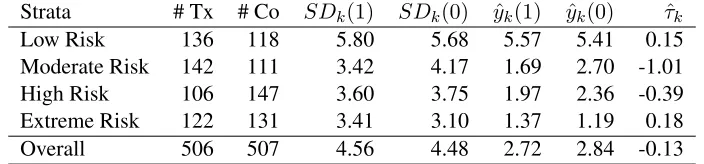
This analysis is simplified for the purposes of illustration. We are only looking at one of the outcomes and have dropped several potentially important covariates for the sake of clarity. Statistics on the strata forK= 4are listed on Table 1. A higher proportion of subjects in the first two groups were treated than one would expect given the randomization. Imbalance in the first group, with its high average outcome, could heavily influence the overall treatment effect estimate ofτˆsd.

Strata # Tx # Co SDk(1) SDk(0) yˆk(1) yˆk(0) τˆk

Low Risk 136 118 5.80 5.68 5.57 5.41 0.15

Moderate Risk 142 111 3.42 4.17 1.69 2.70 -1.01

High Risk 106 147 3.60 3.75 1.97 2.36 -0.39

Extreme Risk 122 131 3.41 3.10 1.37 1.19 0.18

Overall 506 507 4.56 4.48 2.72 2.84 -0.13

Table 1: Strata-Level Statistics for the PAC Illustration

We estimate the minimum gain in precision due to post-stratification by calculating point esti-mates of all the within- and between-strata variances and the between-strata covariance and plugging these values into Equation 9. We are not taking the variability of these estimates into account. By assuming the strata rk are maximal, i.e.,rk = 1 for allk, we estimate a lower bound on the

re-duction in variance due to post-stratification. Theβ’s are estimated by numerical simulation of the randomization process (with 50,000 trials) and are therefore exact up to uncertainty in this Monte Carlo calculation; these values do not depend on the population characteristics and so there is no sampling variability here. We show the resulting estimates for several different stratifications. For

K = 4, we estimate the percent reduction of variance,100%×(Var[ˆτps]−Var[ˆτsd])/Var[ˆτsd], to be

no less than 12%. If the truerkwere less than 1, the benefit would be greater. More strata appear

somewhat superior, but gains level off rather quickly. See Table 2.

The estimate of treatment effect changes markedly under post-stratification. The estimatesτˆps

hover around−0.28 forK = 4and higher, as compared to the−0.13from the simple-difference estimator. The post-stratified estimator appears to be correcting the bias from the random imbalance in treatment assignment.

We can also estimate the MSE for both the simple-difference and post-stratified estimator condi-tioned on the imbalance by plugging point estimates for the population parameters into Equation 15 and Equation 14. We again assume the correlationsrkare maximal. We estimate bias by plugging in

the estimatedyˆk(`)for the mean potential outcomes of the strata. These results are the last columns

of Table 2; the percentage gain in this case is higher primarily due to the correction of the bias term from the imbalance. When conditioning on the imbalanceW, the estimated MSE (i.e., variance) of the post-stratified estimator is slightly higher than thevarianceof the simple-difference estimator, but is substantially lower than its overall MSE. This is due to the bias correction. Because the true variances and therkfor strata are unknown, these gains are estimates only. They do, however,

area of future work.

Uncond. Variance MSE Conditioned onW

K τˆps τˆsd ˆτps τˆsd % MSEτˆps varˆτsd biasτˆsd MSEτˆsd %

2 -0.34 -0.13 0.077 0.081 5% 0.077 0.076 0.207 0.118 35%

4 -0.27 -0.13 0.071 0.081 12% 0.072 0.070 0.137 0.089 19%

10 -0.25 -0.13 0.070 0.081 14% 0.071 0.069 0.119 0.083 15%

15 -0.24 -0.13 0.070 0.081 14% 0.070 0.067 0.115 0.081 13%

30 -0.28 -0.13 0.069 0.081 15% 0.068 0.064 0.148 0.086 21%

50 -0.32 -0.13 0.068 0.081 15% 0.066 0.061 0.190 0.097 32%

Table 2: Estimated Standard Errors for PAC. Table shows both conditioned and unconditioned estimates for different numbers of strata. ‘%’ denotes percent variance reduction.

Matched Pairs Estimation. We can also estimate the gains by building a fake set of potential outcomes by matching treated units to control units on observed covariates. We match as described in Sekhon and Grieve (2011). We then consider each matched pair a single unit with two potential outcomes. We use this synthetic set to calculate the variances of the estimators using the formula from Section 2.

Matching treatment to controls and controls to treatment gives 1013 observations with all poten-tial outcomes “known.” The correlation of potenpoten-tial outcomes is 0.21 across all strata.τ =−0.031. The unconditional variance for the simple-difference and post-stratified estimators are 0.048 and 0.038, respectively. The percent reduction in variance due to post-stratification is 19.6%.

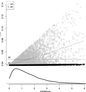
We can use this data set to further explore the impact of conditioning. Assume the treatment probability isp= 0.5and repeatedly randomly assign a treatment vector and compute the resulting conditional MSE. Also compute the “imbalance score” for the treatment vector with a chi-squared statistic:

Imbalance≡X

k

(Wk(1)−pnk)2

pnk

This procedure produces Figure 1. As imbalance increases, the MSE (variance) ofˆτpssteadily, but

slowly, increases as well. The MSE ofτˆpsis quite resistant to large imbalance. This is not the case

forτˆsd, however. Generally, high imbalance means high conditional MSE. This is due to the bias

term which can get exceedingly large if there is imbalance between different heterogeneous strata. Also, for a given imbalance, the simple-difference estimator can vary widely depending on whether stratum-level bias terms are canceling out or not. This variability is not apparent for the post-stratified estimator, where only the number of units treated drives the variance; the post-post-stratified points cluster closely to their trend line.

The curve at the bottom shows the density of the realized imbalance score: there is a good chance of a fairly even split with low imbalance. In these cases, the variance of τˆsd is smaller

than the unconditional formula would suggest. If the randomization turns out to be “typical” the unconditional variance formula would be conservative. If the imbalance is large, however, the unconditional variance may be overly optimistic. This chance of large imbalance with large bias is why the unconditioned MSE ofτˆsdis larger than that ofτˆps.

The observed imbalance for the actual assignment was about 2.37. The conditional MSE is 0.083 forτˆsdand 0.039 forτˆps, a 53% reduction in variance. The conditional MSE for the

Figure 1: PAC MSE Conditioned on Imbalance. Uses constructed matched PAC dataset. Points indicate the conditional MSE ofτˆpsandτˆsd given various specific splits ofW. x-axis is the

imbal-ance score for the split. Curved dashed lines interpolate point clouds. Horizontal dashed lines mark unconditional variances for the two estimators. The curve at bottom is the density of the imbalance statistic.

observed, quite imbalanced, splitW. For the post-stratified estimator, however, the conditional vari-ance is only about 1% higher than the unconditional; the degree of imbalvari-ance is not meaningfully impacting the precision. Generally, with post-stratification, the choice of using an unconditional or conditional formula is less of a concern.

8

Conclusions

Post-stratification is a viable approach to experimental design in circumstances where blocking is not feasible. If the stratification variable is determined beforehand, post-stratification is nearly as efficient as a randomized block trial would have been: the difference in variances between post-stratification and blocking is a smallO(1/n2). However, the more strata, the larger the potential penalty for post-stratification. There is no guarantee of gains.

Conditioning on the observed distribution of treatment across strata allows for a more appropri-ate assessment of precision. Most often the observed balance will be good, even in moderappropri-ate-sized experiments, and the conditional variance of both the post-stratified and simple-difference estimator will be smaller than estimated by the unconditional formula. However, when balance is poor, the conditional variance of the estimators, especially for the simple-difference estimator, may be far larger than what the unconditional formula would suggest. Furthermore, in the unbalanced case, if a truly prognostic covariate is available post-stratification can significantly improve the precision of one’s estimate. For a covariate unrelated to outcome, however, a simple-difference estimator can be superior.

When viewing a post-stratified or a blocked estimate as an estimate of the PATE, under the assumption that the sample is a draw from a larger population, our findings generally hold although the potential for decreased precision is reduced. However, in most cases the sample in a randomized trial is not such a random draw. We therefore advocate for viewing the estimators as estimating the SATE, not the PATE.

Problems arise when stratification is determined after treatment assignment. The results of this paper assume that the stratification is based on a fixed and defined covariateb. However, in practice covariate selection is often done after-the-fact in part because, as is pointed out by Pocock et al. (2002), it is often quite difficult to know which of a set of covariates are significantly prognostic

a priori. But variable selection invites fishing expeditions, which undermine the credibility of any findings. Doing variable selection in a principled manner is still notoriously difficult, and is often poorly implemented; Pocock et al. (2002), for example, found that many clinical trial analyses select variables inappropriately. Tsiatis et al. (2008) summarized the controversy in the literature and, in an attempt to move away from strong modeling, and to allow for free model selection, proposed a semiparametic approach as a solution.

Beach and Meier (1989) suggested that, at minimum, all potential covariates for an experiment be listed in the original protocol. Call thesez. In our framework, variable-selection is then tobuilda stratificationbfromzandT after having randomized units into treatment and control. Stratification

b(now B) is random as it depends onT. Questions immediately arise: how does one define the variance of the estimator? Can substantial bias be introduced by the strata-building process? The key to these questions likely depends on appropriately conditioning on both the final, observed, strata and the process of constructingB. This is an important area of future work.

9

Appendix A

Theorem 2.1. The proof of Theorem 2.1 is based on iterated expectations and a lot of unpleasant algebra. The following shows the highlights. We leave the conditioning on D implicitly in the expectations for cleaner presentation. See the supplementary material for a version with more detail. We first set up a few simple expectations. Under Assignment Symmetry,

E

Ti

Wk(1)

=E E

Ti

Wk(1)

|Wk(1)

=E

1 nk

= 1 nk

Rearrangeβ1k≡E[Wk(0)/Wk(1)] =nkE[1/Wk(1)]−1to getE[1/Wk(1)] = (β1k+ 1)/nkand

E

T2 i

W_k2(1)

=E E

Ti

W_k2(1)|Wk(1)

= 1 nk E

1 Wk(1)

= β1k+ 1

n2_k . (19)

These derivations are easier if we useα1k ≡ E[1/Wk(1)], but the β’s are more interpretable and

lead to nicer final formula. There are analogous formula for the control unit terms and cross terms. We use these relationships to compute means and variances for the strata-level estimators.

Unbiasedness. The strata-level estimators are unbiased:

E[ˆτk] = E



 X

i:bi=k

Ti

Wk(1)

yi(1)− X

i:bi=k

1−Ti

Wk(0)

yi(0) 



= X

i:bi=k

E

Ti

Wk(1)

yi(1)− X

i:bi=k

E

1−Ti

Wk(0)

yi(0)

= X

i:bi=k

1 nk

yi(1)− X

i:bi=k

1 nk

yi(0) =τk.

Variance. Var[ˆτk] =Eτˆk2

−τ_k2. Expandτ_k2into three parts(a)0−(b)0+ (c)0:

τ_k2 =



 X

i:bi=k

1 nk

yi(1) 

 2

| {z }

(a0₎

−2



 X

i:bi=k

1 nk

yi(1) 

 

 X

i:bi=k

1 nk

yi(0) 



| {z }

(b0₎

+



 X

i:bi=k

1 nk

yi(0) 

 2

| {z }

(c0₎

.

Similarly, expand the square ofEˆτk2

to get(a)−(b) + (c). Simplify these parts with algebra and relationships such as shown in Equation 19. We then get, for example

(a) =E



 X

i:bi=k

Ti

Wk(1)

yi(1) 

 2

= β1k+ 1 n2

k

X

i:bi=k

y2_i(1) + −β1k+nk−1 n2

k(nk−1)

X

i6=j

yi(1)yi(1).

Part(b)and(c)are similar.

The variance is then Var[ˆτk] = (a)−(a0)−(b) + (b0) + (c)−(c0), a sum of several ugly

differences. Algebra, and recognizing formulas for the sample variances and covariances, gives:

(a)−(a0) = β1k nk

σ2_k(1)

(b0)−(b) = 2 nk

γk(1,0)

and

(c)−(c0) = β0k nk

σ2_k(0)

Theorem 2.2 The mean is immediate. For the variance, observe:

Var[ˆτps] =E

  K X k=1 nk

n (ˆτk−τk)

!2

 = K X k=1 n_k n 2 E h

(ˆτk−τk)2 i

+X

k6=r

nknr

n2 E[(ˆτk−τk) (ˆτr−τr)].

The first sum is what we want. The second is 0 since, using the tower property and Assignment Symmetry

E[E[(ˆτk−τk) (ˆτr−τr)|W]] =E[E[(ˆτk−τk)|W]E[(ˆτr−τr)|W]] =E[0·0] = 0.

Theorem 4.1. Calculate the MSE ofˆτsdconditioned on the splitW with a slight modification to

the above derivation. Define a new estimator that is a weighted difference in means:

ˆ αk≡Ak

X

i:bi=k

Ti

Wk(1)

yi(1)−Bk X

i:bi=k

1−Ti

Wk(0)

yi(0)

withAk, Bk constant. αˆk is an unbiased estimator of the difference in means weighted byAkand

Bk:

E[ ˆαk] =E



A_k X

i:bi=b

Ti

Wk(1)

yi(1)−Bk X

i:bi=b

Tk

Wi(0)

yi(0) 

=A_ky¯_k(1)−B_ky¯_k(0).

Now follow the derivation of the variance ofˆτkpropagatingAkandBkthrough. These are constant

and they come out, giving

Var[ ˆαk] =

1 nk

A2_kβ1kσk2(1) +Bk2β0kσ2k(0) + 2AkBkγk(1,0)

.

Expandτˆsdinto strata terms:

ˆ τsd=

K X k=1   W1k W1 X

i:bi=k

Ti

W1k

yi(1)−

W0k

W0 X

i:bi=k

1−Ti

W0k

yi(0)  = K X k=1 ˆ αk

withAk=W1k/W1andBk=W0k/W0. Conditioning onW makes theAkand theBkconstants,

β1k=W0k/W1k, andβ0k=W1k/W0k. Assignment symmetry ensures that, conditional onW, the

stratum assignment patterns are independent, so theαˆkare as well, and the variances then add:

Var[ˆτsd|W] = K X

k=1

Var[ ˆαk|W].

The bias isE[ˆτsd|W]−τ with

E[ˆτsd|W] = K X

k=1

E[ ˆαk|W] = K X

k=1

Aky¯k(1)−Bky¯k(0).