Stochastic Solvency Testing in Life Insurance

(1)

Stochastic Solvency Testing

in Life Insurance

Genevieve Katherine Hayes

A thesis submitted for the degree of Doctor of Philosophy of

The Australian National University

(2)

(3)

Statement of Originality

This thesis contains no material that has been accepted for the award of any other degree or diploma in any University, and to the best of my knowledge and belief, contains no material published or written by another person, except where due reference is made in the thesis.

Genevieve Hayes

September 2008

(4)

(5)

Acknowledgements

Over the course of my PhD, I have received advice and direction from a number of people, first among them being Prof. Ross Maller. Ross taught me the importance of statistical evidence in justifying opinions, no matter how wise they may appear. I have never met anyone with higher standards than Ross, both of himself and of his students, and although, at times, I wished that he would lower these standards, I am now glad that he never did. I could not imagine a better supervisor than Ross. I would also like to thank Dr. Steven Stern, David Service, Aaron Bruhn, Adam Butt, Tim Higgins, Jeff Dukes, Sue Howes, Winnie Luo and Prof. David Wilkie, for their assistance and feedback.

Thank you to the Australian National University School of Finance and Applied Statistics for providing me with the resources necessary to complete my research, and to the following individuals for assisting me in gaining access to the data used in this thesis: Dr. Len Smith of the Australian Centre for Population Research at the Australian National University, who provided access to the Australian Population Data Set; Anthony Brien and Sue Clark of the Institute of Actuaries of Australia Life Risk Insurance Committee, who provided access to the IAAust Data Set; and the Australian Life Insurer (which must remain anonymous for confidentiality reasons) that supplied the Single Insurer Data Set.

Finally, I would like to thank my parents, who lived through this PhD with me. They never stopped believing in me, even on those occasions when I thought that I would never make it to the end of it all.

(6)

(7)

Abstract

Stochastic solvency testing methods have existed for more than 20 years, yet there has been little research conducted in this area, particularly in Australia. This is for a number of reasons, the most pertinent of which being the lack of computing capabilities available in the past to implement more sophisticated techniques. How-ever, recent advances in computing have made stochastic solvency testing possible in practice and have resulted in a trend towards this being done in advanced studies. The purpose of this thesis is to develop a realistic solvency testing model in a form that can be implemented by Australian Life Insurers, in anticipation that the Australian insurance regulator, APRA, will ultimately follow the world trend and require stochastic solvency testing to be carried out in Australia. The model is constructed from three interconnected stochastic sub-models used to describe the economic environment and the mortality and lapsation experience of the portfolio of policies under consideration. Australian economic and Life Insurance data is used to fit a number of possible sub-models, such as generalised linear models, over-dispersion models and asset models, and the “best” model is selected in each case. The selected models are a modified CAS/SOA economic sub-model; either a Poisson or negative binomial (NB1) distribution (depending on the policy type considered) as the mortality sub-model; and a normal-Poisson lapsation sub-model.

Based on tests carried out using this model, it is demonstrated that, for portfolios of level and yearly-renewable term insurance business, the current deterministic solvency capital requirements provide little protection against insolvency. In fact, for the test portfolios of term insurance policies considered, the deterministic capital requirements have levels of sufficiency of less than 2% (on a Value at Risk basis) when compared to the change in capital distribution over a three year time horizon. This is of concern, as yearly-renewable term insurance comprises a significant volume of Life Insurance business in Australia, with there being over 426,000 yearly-renewable

(8)

vi

term insurance policies on the books of Australian Life Insurers in 1999 and more business expected since then.

(9)

List of Tables

4.1 A Comparison of Reduction Factors at Selected Ages . . . 38

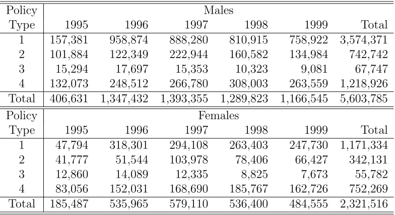
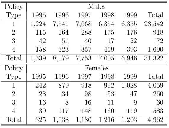
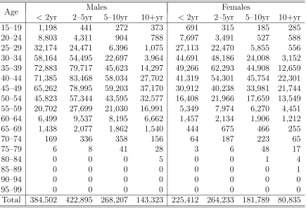
5.1 Exposures by Sex, Policy Type and Year . . . 50 5.2 Deaths by Sex, Policy Type and Year . . . 51

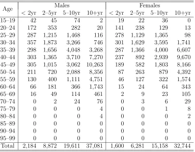
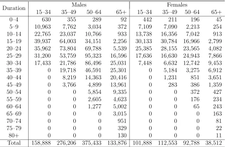
5.3 Exposures by Age Band, Sex and Duration Band for Type 1 Policies 51 5.4 Exposures by Age Band, Sex and Duration Band for Type 2 Policies 52

5.7 Exposures by Sex, Policy Type and Year . . . 55 5.8 Deaths by Sex, Policy Type and Year . . . 55

5.9 Non-Death Terminations by Sex, Policy Type and Year . . . 56

5.12 Exposures as a % of the Total for each Policy Type/Sex/Data Set Combination by Age Band . . . 57 5.13 Exposures as a % of the Total for each Policy Type/Sex/Data Set

Combination by Duration Band . . . 58

5.14 Exposures and Withdrawals by Policy Type and Year . . . 59 5.15 Exposures by Duration Band and Policy Type . . . 60

5.16 Exposures as a % of the Total for each Policy Type by Duration Band 60 5.17 A Summary of the Economic Data . . . 62

5.18 Summary Statistics for the Economic Data . . . 63 5.19 Correlations Between the Economic Variables withp-values Shown in

Brackets . . . 67

(16)

xiv LIST OF TABLES

6.1 Correlations Between Mortality Ratios and Lapse Ratios by Lag, Sex and Policy Type (All Ages) withp-values Shown in Brackets . . . 76 6.2 Correlations Between Mortality Ratios and Lapse Ratios by Lag, Sex

and Policy Type (Ages 15–64 Only) with p-values Shown in Brackets 76 6.3 Drop in Deviance Between the Two Selective Lapsation GLMs by

Maximum Lag . . . 77 6.4 Correlations Between Insured Life Mortality Ratios and Economic

Variables (1995–1999) withp-values Shown in Brackets . . . 89 6.5 Correlations Between Population Mortality Ratios and Economic

Vari-ables with p-values Shown in Brackets . . . 91 6.6 Drop in Deviance between the Two Economic Fluctuation versus

Mortality GLMs . . . 93 6.7 Analysis of Deviance Table for Model 2 for the IAAust Data . . . 93 6.8 Fitted Coefficients for the Economic Fluctuation versus Mortality

GLMs with Standard Errors Shown in Brackets . . . 94 6.9 % Change in the Mortality Ratio Associated with a 1% Change in

the Short-Term Interest Rate . . . 95 6.10 Correlations Between (All-Duration) Lapse Ratios and Economic

Vari-ables (Single Insurer Mortality Data) with p-values Shown in Brackets 101 6.11 Correlations Between (All-Duration) Lapse Ratios and Economic

Vari-ables (Single Insurer Lapsation Data) withp-values Shown in Brackets 101 6.12 Decrease in Deviance between the Two Economic Fluctuation versus

Mortality GLMs . . . 102 6.13 Fitted Coefficients for the Economic Fluctuation versus Mortality

GLMs (Model 2) with Standard Errors Shown in Brackets . . . 103 6.14 % Change in the Lapsation Ratio Associated with a 1% Change in

Each of the Economic Variables for the Single Insurer Mortality Data 103

7.1 Fitted Parameter Values for the Kemp Model with Standard Errors Shown in Brackets . . . 121 7.2 Correlation Matrix for the Kemp Model withp-values Shown in

Brack-ets . . . 121 7.3 Goodness of Fit Statistics for the Kemp Random Walk Model . . . . 122 7.4 A Summary of the Wilkie Model Sub-Models Used in this Thesis . . 124 7.5 Fitted Parameter Values for the Wilkie Model . . . 124 7.6 Goodness of Fit Statistics for the Wilkie Model Time Series Processes 124 7.7 Fitted Parameter Values for the CAS/SOA Model . . . 126 7.8 Goodness of Fit Statistics for the CAS/SOA Model Time Series

(17)

LIST OF TABLES xv

7.9 A Comparison of the AIC for the Kemp, Wilkie and CAS/SOA

Mod-els . . . 127

7.10 Fitted Parameter Values for the Modified CAS/SOA Model . . . 129

7.11 Goodness of Fit Statistics for the Modified CAS/SOA Model . . . . 129

7.12 A Summary of the Over-Dispersion Models Fitted to the Data . . . 133

7.13 Over-Dispersion Statistics for the Poisson GLMs withp-values Shown in Brackets . . . 134

7.14 Over-Dispersion Parameters for the Over-Dispersion Models with p -values Shown in Brackets . . . 135

7.15 AIC for the Models Fitted to the Type 1 Males and Females Data . 137 7.16 Fitted Coefficients for the Over-Dispersion Models with Standard Er-rors Shown in Brackets . . . 137

7.17 Over-Dispersion Statistics for the Lapsation Data Poisson GLMs with p-values Shown in Brackets . . . 140

7.18 Over-Dispersion Parameters for the Lapsation Over-Dispersion Mod-els with p-values Shown in Brackets . . . 141

7.19 AIC for the Lapsation Over-Dispersion Models . . . 142

7.20 Fitted Coefficients for the Normal-Poisson Random Coefficient Model with Standard Errors Shown in Brackets . . . 144

7.21 Fitted Variances and Covariances for the Normal-Poisson Random Coefficient Model with Standard Errors Shown in Brackets . . . 144

8.1 Model Portfolio Compositions . . . 161

8.2 Duration Assumptions (Years) by Age Band, Sex and Policy Type . 162 8.3 Expense Assumptions per Policy . . . 163

8.4 Composition of each of the Model Asset Portfolios . . . 164

8.5 Regular Annual Premiums Assumed for Type 1 and 3 Policies by Age Band . . . 167

8.6 Single Premiums Assumed for the Type 2 (M and F) Policies Under Each Investment Option by Age Band . . . 168

8.7 Implicit Profit Margins (% of After-Tax Investment Earnings) for Type 2 Policies Under Each Investment Option . . . 168

8.8 Premium Rate Scale for Type 4 Policies ($) . . . 170

8.9 Implicit Profit Margins (% of Claims) for Type 4 Policies . . . 170

8.10 Economic Variable Starting Values . . . 171

(18)

xvi LIST OF TABLES

8.14 Selected Capital Adequacy Margins . . . 177

8.15 Fitted Values of αd and αw by Policy Type and Sex . . . 181

9.1 VaR and TVaR Per Policy for the Base Case Scenarios ($) . . . 185

9.2 Best Estimate Liabilities, and Solvency and Capital Adequacy Capi-tal Requirements Per Policy for the Base Case Scenarios ($) . . . 186

9.3 Levels of Sufficiency (on a VaR Basis) of the LPS2.04 and LPS3.04 Capital Requirements for the Base Case Scenarios . . . 187

9.4 Summary Statistics for the Base Case Simulations . . . 187 9.5 Number of Iterations Performed, the Time Required and the Number

of Iterations Needed for Convergence for the Base Case Scenarios . . 188

9.6 p-values for the Kolmogorov-Smirnov and Anderson-Darling Tests for the Base Case Scenarios . . . 189

9.7 Stochastic Minimum Asset Requirements for the Base Case Scenarios ($) . . . 190 9.8 Ratios of the LPS2.04 and LPS3.04 Solvency and Capital Adequacy

Requirements to the Stochastic Minimum Asset Requirements for the Base Case Scenarios . . . 191

9.9 p-values for the Two-Sample Kolmogorov-Smirnov Tests for the Eco-nomic Sub-Model Sensitivity Scenarios . . . 193

9.10 VaR and TVaR Per Policy for the Economic Sub-Model Sensitivity Analysis Scenarios ($) with Ratios of these Amounts to the Base Case Capital Requirements Shown in Brackets . . . 195 9.11 Best Estimate Liabilities, and Solvency and Capital Adequacy

Capi-tal Requirements Per Policy for the Economic Sub-Model Sensitivity Analysis Scenarios ($) . . . 196

9.12 Levels of Sufficiency (on a VaR Basis) of the LPS2.04 and LPS3.04 Capital Amounts for the Economic Sub-Model Sensitivity Analysis Type 3 and 4 Policy Scenarios . . . 197 9.13 Ratios of the Economic Sub-Model Sensitivity Analysis Stochastic

Minimum Asset Requirements to the Base Case Requirements for the Same Portfolio . . . 198

9.14 Summary Statistics for the ₋∆C(1) and ₋∆Cmin(0,3) Simulations

for the Economic Sub-Model Sensitivity Analysis Scenarios . . . 199

9.15 p-values for the Kolmogorov-Smirnov and Anderson-Darling Tests for the Economic Sub-Model Sensitivity Analysis Scenarios . . . 200

(19)

LIST OF TABLES xvii

9.17 p-values for the Two-Sample Kolmogorov-Smirnov Tests for the

Lap-sation Sub-Model Sensitivity Scenarios . . . 202

9.18 VaR and TVaR Per Policy for the Lapsation Sub-Model Sensitivity Analysis Scenarios ($) with Ratios of these Amounts to the Economic Base Case Capital Requirements Shown in Brackets . . . 203

9.19 p-values for the Two-Sample Kolmogorov-Smirnov Tests for the Mor-tality and Lapsation Sub-Model Sensitivity Scenarios . . . 204

9.20 p-values for the Two-Sample Kolmogorov-Smirnov Tests for the De-pendencies Sensitivity Scenarios . . . 206

9.21 VaR and TVaR Per Policy for the Dependencies Sensitivity Analysis Scenarios ($) with Ratios of these Amounts to the Economic Base Case Capital Requirements Shown in Brackets . . . 208

9.22 p-values for the Two-Sample Kolmogorov-Smirnov Tests for the Dis-tributional Mean Sensitivity Analysis Scenarios . . . 210

9.23 VaR and TVaR Per Policy for the Distributional Mean Sensitivity Analysis Scenarios ($) with Ratios of these Amounts to the Economic Base Case Capital Requirements Shown in Brackets . . . 212

9.24 Ratios of the Distributional Mean Sensitivity Analysis Stochastic Minimum Asset Requirements to the Economic Base Case Require-ments for the Same Portfolio . . . 213

9.25 Ratios of the Distributional Mean Sensitivity Analysis Stochastic Minimum Asset Requirements to the (Original) Base Case Require-ments for the Same Portfolio . . . 215

9.26 Average Numbers of Iterations Required for Simulation Convergence and Accuracy . . . 217

A.1 IA95-97 M and F . . . 226

A.2 ALT95-97 M and F . . . 227

A.3 Mortality Reduction Factors. . . 228

A.4 Expected Lapse Rates by Curtate Duration (Years) and Policy Type. 229 D.1 Stochastic Minimum Asset Requirements for the Economic Sub-Model Sensitivity Analysis Scenarios ($) . . . 240

D.2 Ratios of the LPS2.04 Solvency Requirements to the Stochastic Min-imum Asset Requirements for the Economic Sub-Model Sensitivity Analysis Scenarios . . . 241

(20)

xviii LIST OF TABLES

D.4 Summary Statistics for the ₋∆C(1) and ₋∆Cmin(0,3) Simulations

for the Mortality Sub-Model Sensitivity Analysis Scenarios . . . 243 D.5 Summary Statistics for the ₋∆C(1) and ₋∆Cmin(0,3) Simulations

for the Lapsation Sub-Model Sensitivity Analysis Scenarios . . . 244 D.6 Levels of Sufficiency (on a VaR Basis) of the LPS2.04 and LPS3.04

Capital Amounts for the Lapsation Sub-Model Sensitivity Analysis Scenarios . . . 245

D.7 Stochastic Minimum Asset Requirements for the Lapsation Sub-Model Sensitivity Analysis Scenarios ($) . . . 245 D.8 p-values for the Kolmogorov-Smirnov and Anderson-Darling Tests for

the Lapsation Sub-Model Sensitivity Analysis Scenarios . . . 245 D.9 Summary Statistics for the ₋∆C(1) and ₋∆Cmin(0,3) Simulations

for the Mortality and Lapsation Sub-Model Sensitivity Analysis Sce-narios . . . 246 D.10 Summary Statistics for the ₋∆C(1) and ₋∆Cmin(0,3) Simulations

for the Dependencies Sensitivity Analysis Scenarios . . . 247

D.11 Best Estimate Liabilities, and Solvency and Capital Adequacy Capi-tal Requirements Per Policy for the Dependencies Sensitivity Analysis Scenarios ($) . . . 248

D.12 Levels of Sufficiency (on a VaR Basis) of the LPS2.04 and LPS3.04 Capital Amounts for the Dependencies Sensitivity Analysis Scenarios 249 D.13 Stochastic Minimum Asset Requirements for the Dependencies

Sen-sitivity Analysis Scenarios ($) . . . 250 D.14 Ratios of the LPS2.04 and LPS3.04 Requirements to the Stochastic

Minimum Asset Requirements for the Dependencies Sensitivity Anal-ysis Scenarios . . . 251 D.15p-values for the Kolmogorov-Smirnov and Anderson-Darling Tests for

the Dependencies Sensitivity Analysis Scenarios . . . 252

D.16 Summary Statistics for the ₋∆C(1) and ₋∆Cmin(0,3) Simulations

for the Distributional Mean Sensitivity Analysis Scenarios . . . 253 D.17 Best Estimate Liabilities, and Solvency and Capital Adequacy

Capi-tal Requirements Per Policy for the Distributional Mean Sub-Model Sensitivity Analysis Scenarios ($) . . . 254 D.18 Stochastic Minimum Asset Requirements for the Distributional Mean

Sensitivity Analysis Scenarios ($) . . . 255 D.19 Ratios of the LPS2.04 Solvency Requirements to the Stochastic

(21)

LIST OF TABLES xix

D.20 Ratios of the LPS3.04 Capital Adequacy Requirements to the Stochas-tic Minimum Asset Requirements for the Distributional Mean Sensi-tivity Analysis Scenarios . . . 257 D.21p-values for the Kolmogorov-Smirnov and Anderson-Darling Tests for

(22)

(23)

List of Figures

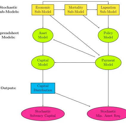
3.1 A Simplified Pictorial View of the Solvency Testing Model Framework 28

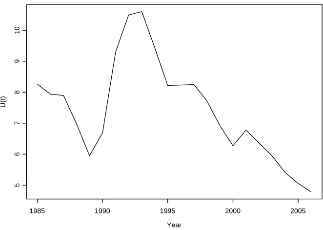
5.1 CPI Inflation (∆ lnQ(t)) . . . 64 5.2 Share Price Index Growth (∆ lnP (t)) . . . 64 5.3 Dividend Yield (lnY (t)) . . . 65 5.4 Interest Rates (ln (1 +R(t)) and ln (1 +F (t))) . . . 65 5.5 Property Yield (∆ lnZ(t)) . . . 66 5.6 Unemployment Rate (U(t)) . . . 66

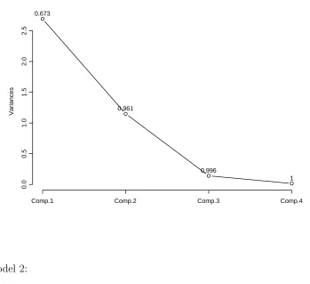
6.1 A Scree Plot for the Economic Data. . . 87

6.2 All-Age All-Duration Mortality Ratios for the IAAust Data Set . . . 88 6.3 All-Age Mortality Ratios for the Australian Population Data Set . . 90

6.4 All-Age Mortality Ratios versus Short-Term Interest Rate (%) for the Australian Population Data Set . . . 91

6.5 All-Age Mortality Ratios versus Unemployment Rate (%) for the Aus-tralian Population Data Set . . . 92 6.6 All-Age, All-Duration Insured Life Lapse Ratios (Single Insurer

Mor-tality Data) . . . 100

6.7 All-Duration Insured Life Lapse Ratios (Single Insurer Lapse Data) . 100

7.1 Relationships Between the Variables in the Wilkie Model . . . 110

7.2 Relationships Between the Variables in the CAS/SOA Model . . . . 112

7.3 Property Yield Correlogram (∆ lnZ(t)) . . . 120 7.4 A Simplified Pictorial View of the Stochastic Sub-Model Cascade

Structure . . . 145

(24)

xxii LIST OF FIGURES

(25)

CHAPTER

1

Introduction

The most important goal of any business is to remain solvent, as it can no longer continue its operations if it becomes insolvent, except in special circumstances where the government bails out the company by injecting capital. In the case of financial services institutions, such as banks and insurance companies, continued solvency is of importance, not just to the institution, but also to account/policyholders who could potentially face economic hardship if such an institution were to collapse. The 2001 collapse of Australian General Insurer HIH Insurance illustrates the adverse consequences to the public of such an event. As a result, the financial services in-dustry is one of the most highly regulated industries, and all advanced economies have in place legislation designed to minimise the risk of a financial services insti-tution going bankrupt. The legislation generally requires such instiinsti-tutions to hold capital greater than a specified minimum amount, often referred to as the solvency capital requirement, at all points in time. This thesis focuses on the calculation of this quantity in the context of the Australian Life Insurance industry.

Currently, Australian Life Insurers are required to calculate their solvency cap-ital requirements on a deterministic basis using formulae set out in Life Insurance Prudential Standards LPS2.04 and LPS3.041_{. However, recently there has been a} trend in advanced economies, such as Switzerland, through the Swiss Solvency Test, and the European Union countries, through Solvency II, towards calculating insurer

1_{LPS2.04 and LPS3.04 specify methodologies the insurer must follow in order to determine its}

solvency and capital adequacy requirements, respectively. The insurer must hold assets greater than both of these requirements at all times. If the insurer’s assets fall below the solvency require-ment, the insurer is considered to be insolvent for statutory purposes, while if its assets fall below the capital adequacy requirement, the Australian insurance regulator, the Australian Prudential Regulatory Authority (APRA), will intervene in the hope of preventing the insurer from becoming insolvent.

(26)

2 Introduction

solvency capital requirements using stochastic techniques, thereby requiring insurers to hold a capital amount that satisfies a probability-based criterion. For example, insurers might be required to hold an amount of capital sufficiently large so that there is a 99.5% chance that, in one year’s time, the insurer’s assets will exceed its liabilities. In order to satisfy such a criterion, the insurer must attempt to determine the probability distributions of the values of its assets and liabilities, or sometimes just of its capital holdings, at future points in time. These distributions usually need to be determined using computer-intensive simulation techniques. It was due to the unavailability of inexpensive, high-speed computers in the past that determin-istic solvency testing techniques were used almost exclusively in all countries, and it is because of the easier access to such computers in recent years that stochastic solvency testing techniques have suddenly come to prominence.

It is anticipated that the Australian insurance regulator, the Australian Pruden-tial Regulatory Authority (APRA), will ultimately require Australian Life Insurers to calculate their solvency capital requirements using stochastic methods. Such be-ing the case, there is a need to develop a realistic asset-liability model that can be used for this purpose. In this thesis, such a model is constructed and the model is then used to assess whether the current Australian deterministic solvency capital criteria are appropriate, based on four commonly used stochastic solvency criteria: the 99.5% Value at Risk (VaR) and Tail Value at Risk (TVaR) of the change in capital distribution over a one year time horizon, and the 95% VaR and TVaR of the change in capital distribution over a three year time horizon. The developed model is a simulation model comprising three interconnected stochastic sub-models used to describe the economic environment and the mortality and lapsation experi-ence. It is demonstrated, using Australian economic and Life Insurance data, that the “best” sub-model in each case (out of the range of models under consideration) is a modified CAS/SOA2 _{economic sub-model, a Poisson or negative binomial} (de-pending on the policy type considered) mortality sub-model, and a normal-Poisson lapsation sub-model.

Tests conducted in this thesis demonstrate that, although the current determin-istic requirements are sufficiently high for portfolios of investment-linked or “tradi-tional” (endowment insurance) policies, they provide very little protection against insolvency for portfolios of “traditional” term insurance or for portfolios of “mod-ern” yearly-renewable term insurance under some of the solvency criteria. Sensitivity tests conducted in association with these investigations show that the (stochastic) total asset requirements calculated using the solvency testing model are virtually un-affected by ignoring the over-dispersion that was found to be present in the mortality and lapsation data used in this thesis, or dependency relationships that were found

(27)

Introduction 3

to exist between the economy and mortality rates, and the economy and lapsation rates. However, for some policy types, the requirements are significantly affected by changing the sub-model used to forecast the economic variables, or simplifying the formulae used to determine the mean mortality and lapsation rates in the sub-models used to forecast future mortality and lapsation experience. The implication of this latter result is that, if APRA is to require Life Insurers to calculate their solvency capital requirements using stochastic methods, then, in order to ensure consistency between insurers, some guidance should be provided with regard to the nature of the solvency testing model used.

(28)

(29)

CHAPTER

2

Life Insurance Solvency Testing: A Review

2.1 Introduction

In the context of accounting, a business is considered to be solvent if it can pay its debts as they fall due. Thus, a business is generally considered to be solvent if its assets exceed its liabilities. The difference between assets and liabilities is referred to as capital. In the context of insurance, however, the values of the assets and liabilities are uncertain and solvency must be defined in terms of a probability statement. For example, an insurer is considered to be solvent at a particular point in time, t, if there is a sufficiently high probability that the insurer’s assets are greater than its liabilities at that time. That is, for some pre-specified value α,

P r_{A(t)> L(t)_{} ≥}1₋α; (2.1)

where 0< α <1, A(t) denotes the value of the insurer’s assets at time t, and L(t) denotes the value of the insurer’s liabilities at time t. A major proportion of the insurer’s liabilities are policy liabilities (defined in Section 2.2).

In spite of the fact that the insurer’s future assets and liabilities are both stochas-tic quantities, traditionally an insurer’s solvency position has been evaluated using prescribed formulae that ignore the random nature of these amounts, that is, on a deterministic basis. This is primarily due to the lack of computational capabilities required to implement more advanced techniques. However, stochastic asset and liability valuation techniques have existed for the past 25 years1 _{and in recent years,} due to advances in computing, there has been a trend towards stochastic solvency

1_{For example, see Panjer and Bellhouse (1980).}

(30)

6 Life Insurance Solvency Testing: A Review

testing (also referred to as dynamic solvency testing), although this is not, as yet, required by legislation in Australia2_.

The purpose of this chapter is to provide an overview of the techniques currently used in Life Insurance policy liability valuation, and of the current valuation and solvency legislation, as well as a review of the existing stochastic valuation and solvency testing literature with a view to applying it to the Australian insurance environment.

2.2 Reserves and Policy Liabilities

A Life Insurance policy reserve, as defined by Booth et al. (2005, p.223), is “the amount of assets that the Life Office3 _{needs to hold at a particular point in time} (the valuation date) such that, allowing for future premium income and for the anticipated returns from investment, the (insurance) liabilities of the Life Office will be met as they fall due, (where) the (insurance) liabilities of the Life Office can be defined as:

1. The obligations that the company has under the contracts currently in force to pay benefits according to the terms of those contracts.

2. The expenses that the Life Office will incur in the future in order to administer the contracts of insurance it holds.

3. The obligation to provide a return to those with a stake in the company for the capital that they have provided; that is, to the with-profits policyholders and/or shareholders, as appropriate.

4. Taxation.”

The terms policy reserve (or reserve) and policy liability are often used inter-changeably. However, it is important to distinguish between these terms. The policy liability (also termed policy value) for a Life Insurance contract (or block of

2_{Note that the trend towards stochastic solvency testing, referred to in this paragraph, has}

been observed in the legislative standards issued by insurance regulators and not in accounting

standards. AASB 1038, the Australian Accounting Standard which applies to Life Insurance contracts and which is the Australian equivalent to International Financial Reporting Standard IFRS 4, requires a market consistent value to be placed on an insurer’s asset and liabilities at the current reporting date and the insurer’s solvency is determined subject to the standard accounting definition of solvency, given previously. Other advanced economies also have similar accounting standards in place. In this thesis, we focus only on solvency testing from a regulatory point of view.

(31)

Life Insurance Solvency Testing: A Review 7

contracts) which is in force4 _{is the result of the calculation:}

Policy Liability = Expected present value of future outgoings

−Expected present value of future income; (2.2)

while the policy reserve is the amount actually held in respect of a contract and may differ from the theoretical policy value. For example, the reserve may equal the calculated policy liability plus an additional risk margin added to better ensure that the insurer will be able to meet all claim payments even if the actual claims experience turns out to be worse than expected. Policy reserves are calculated for various purposes, including statutory reporting requirements, and in order to calculate the insurer’s future financing requirements. This distinction between these terms is made throughout this thesis.

Equation (2.2) is a prospective formula for calculating policy liabilities (the result of this calculation is often referred to as aprospective policy liability). An alternative approach to calculating policy liabilities is to use a retrospective (or accumulation) approach. Under this approach the (retrospective) policy liability for an in force insurance contract is calculated as:

Policy Liability = Accumulated value of income to date

−Accumulated value of outgoings to date; (2.3) where the accumulated values are calculated allowing for both interest and survivor-ship5_{. If the retrospective and prospective policy liabilities for a given policy at a} given point in time are calculated using the same set of mortality, lapsation and economic assumptions, then they will be equal, but otherwise may differ (Faculty of Actuaries and Institute of Actuaries (2008)).

In practice the prospective method of valuation is most often used, except in the case of unbundled policies (for example, investment-linked policies). However, for consistency, in this thesis we shall use the prospective method to value all policy types. Thus, the term policy liability is taken to refer to the prospective policy liability. Policy liabilities comprise a major proportion of an insurer’s liabilities (the residual liabilities typically being those thatany business entity, not just an insurer, would be expected to hold) and thus, estimating the insurer’s policy liabilities is integral to determining an insurer’s solvency position.

4_{An insurance contract is said to be}_{in force} _{if it has been written, that is, the policy term has}

commenced, and has not yet expired through reaching the end of its term or following a claim, nor has it been terminated by either the insurer or the policyholder.

5

Theaccumulated value allowing for interest and survivorship of $1, invested for a term of n

years at an interest rate ofip.a by a life currently agedxexact, is (1 +i)n/npx, wherenpxdenotes

(32)

2.3 An Overview of Policy Valuation Techniques

Prior to the widespread use of computers, actuaries used very simplistic methods for performing policy valuations. One such method used was the net premium policy valuation method, described in Carr (2004), which makes no explicit allowance for future profit distribution or expenses. Traditional valuation methods, such as the net premium valuation method, were typically implemented using actuarial mathemati-cal formulae6 _{that could be evaluated with the assistance of tabulated commutation} functions7_{, in order to perform the required expected present value calculations.} These formulae required a minimal number of parameters to evaluate (typically only the mortality table, a fixed interest rate and policy details, such as the age of the policyholder, term of the contract and sum insured) and made simplifying assumptions, such as making no allowance for lapsation8_{. Furthermore,} conserva-tive valuation assumptions (for example, a low future interest rate or high mortality rates) were typically used to include an implicit margin against the risk of insol-vency in the policy value. In fact, in Australia, the Life Insurance Act 1945 required the use of conservative valuation assumptions when calculating policy liabilities for statutory reporting purposes.

The advancement of fast, inexpensive computers made possible valuation tech-niques that were previously considered impractical due to the large number of cal-culations involved, in particular, projection (or discounted cashflow) techniques. Projection techniques involve calculating the expected cashflows (for example, of premiums, claims and expenses) for each time period for a policy (or block of poli-cies) and then discounting these cashflows to get the expected present values required in Equation (2.2). Projection techniques are usually implemented using either spe-cialist computer software or spreadsheet models designed to incorporate all of the necessary variables and assumptions. If spreadsheet models are used, as is the case in this thesis, it is common to build two models: a policy model and a payment model. The policy model is used to forecast the number of policies in force at discrete in-tervals in time (usually monthly, half-yearly, or annually) and once the number of policies in force at each point in time is known, the policy cashflows are forecast using the payments model. Some simplifying assumptions are still required in

build-6_{Actuarial mathematical formulae are discussed in detail in most Life Insurance mathematics}

texts, for example Bowers et al. (1997), Gerber (1997) and Promislow (2006).

7

Commutation functions are computational devices developed in the 18th century to assist in the calculation of numerical values for many actuarial quantities, in particular the expected present values of insurance and annuity benefits. Prior to the widespread availability of computers and electronic calculators, values of commutation functions were tabulated for specific interest rates and life tables, for lives of differing ages, thus reducing the time required to calculate premiums and policy values. For further details see Gerber (1997).

8

(33)

ing such models (for example, assumptions are often made concerning the timing of cashflows). Nevertheless, these models allow for additional complexities (such as allowance for withdrawals) not previously feasible with traditional techniques.

With the movement towards projection techniques also came a movement to-wards calculating policy liabilities on a realistic basis; that is, allowing for all rele-vant cashflows and using realistic, rather than conservative, valuation assumptions. Historically, realistic policy liabilities were only used for management information and not in published accounts. However, in recent years most developed countries have incorporated the requirement of realistic policy liabilities for statutory report-ing purposes in their Life Insurance legislation. In Australia, this requirement was incorporated in the Life Insurance Act 1995. To protect against the risk of insol-vency, an explicit risk margin can be added to the realistic policy liability, once it is calculated, to give the amount required for reserving purposes. Such risk margins are also, typically, required by legislation.

In general, the valuation techniques described above are implemented using de-terministic valuation assumptions, that is, all valuation model assumptions are as-sumed to be known (non-random) values, even if this is clearly untrue, as in the case of future interest rates. The only random variables allowed for in a determin-istic valuation are time-until-death and time-until-withdrawal. The distributions of these random variables are summarised in decrement tables of mortality and lap-sation (or lapse) rates. For use in the valuation model, however, the mortality and lapse rates in these tables are assumed to be deterministic. A policy value calculated using deterministic valuation assumptions is referred to as a determin-istic policy value. Determindetermin-istic methods suffice for the calculation of realdetermin-istic (or best estimate) policy values. However, they do not allow for the estimation of the probability distribution of the policy liabilities9_{. Without such an estimate, it is} impossible to determine the probability of adequacy of the policy reserves. To esti-mate the probability distribution of the policy liabilities, it is necessary to employ stochastic valuation techniques.

Stochastic valuation techniques generally involve replacing some of the quantities used in the deterministic valuation assumptions in the previously mentioned meth-ods with random variables. Not all of the quantities need be assumed stochastic (that is, random variables). In some cases, a deterministic assumption is adequate (for example, expense assumptions). Nevertheless, mortality rates, lapsation rates and economic processes such as interest and inflation are generally considered to be stochastic in nature and should be treated accordingly in the valuation. A number of papers have been written suggesting ways in which this can be done; a review is

9_{Historically, to account for variability of estimates, some sensitivity analysis is performed of}

(34)

given in Section 2.5.

By replacing the deterministic assumptions with stochastic ones, the policy value becomes a random variable for which a probability distribution can be estimated. Using this information, it is then possible to determine a best estimate policy liability (usually this is set equal to the mean of the distribution) and to set reserves at a pre-specified level of adequacy (for example, a 75% probability that the reserve is sufficient to meet all future claim payments and policy expenses as they fall due).

Stochastic liability valuation techniques have existed for the past 25 years, but in spite of this, stochastic reserves are rarely calculated in the context of Life Insurance. This is partly due to the lack of computational capabilities required to implement such techniques and a lack of understanding of these techniques by the actuarial community in general. However, it is mainly due to the high level of complexity of this task. To determine the probability distribution of a Life Insurer’s policy liabilities, it is necessary to “determine the sensitivity of the (policy liabilities) to all relevant risk factors over the whole run-off period of the liabilities which (is) often 40 to 50 years” (FOPI (2006, p. 9)), and the resulting distribution depends heavily on the assumptions made in determining it. Nevertheless, it is generally believed the probability distribution of the change in the best estimate policy liability over a relatively short time horizon (for example, one year), required for stochastic solvency testing, can be calculated with reasonable stability, and for this reason, recent ad-vances in computing have resulted in stochastic solvency testing becoming an area of increasing interest to insurers and insurance regulators. Stochastic solvency testing is discussed in the next section.

2.4 Solvency

Estimating the value of policy liabilities is just one step in the process required to assess an insurer’s solvency position. Traditionally, solvency has been assessed on a deterministic basis, by using prescribed formulae that ignore the random nature of the valuation parameters. These formulae are sometimes called “risk-based cap-ital models”. An insurer is considered to be solvent if, at the valuation date, its assets are greater in value than its liabilities (both policy liabilities and non-policy10 liabilities), with sufficient buffer for capital. Policy liabilities are valued using one of the deterministic techniques mentioned in Section 2.3 and conservative valuation assumptions are enforced so as to include an implicit risk margin in the estimate (more recently, an explicit deterministic risk margin was added to the best estimate

10

(35)

of the policy liabilities instead of an implicit margin). In many instances, additional margins are also added to the liabilities to allow for other risks not included in the policy liability risk margin, such as asset risks (for example, credit risk and liquidity risk) and catastrophe risk. That is, an insurer is considered to be solvent if:

A(0)> L(0) + Risk margins, (2.4)

where t = 0 is the valuation date.

As in the case of policy reserving, it is also possible to evaluate an insurer’s solvency position using stochastic techniques. This is referred to in this thesis as stochastic solvency testing. Stochastic solvency testing involves determining proba-bility distributions forA(t) andL(t), or sometimes, just for the insurer’s capital at time t,C(t), where C(t) =A(t)₋L(t), and using these to determine the amount of capital the insurer must hold at the solvency testing date such that a probability-based solvency criterion (for example11_, _{P r}₍_C₍_t₎_>_{0) = 0}_._{995) is satisfied. An} insurer is then considered to be solvent if the amount of capital that it is currently holding is greater than this amount (additional risk margins may also be added to this minimum capital amount, as in the deterministic case).

There are many overlaps between stochastic reserving and stochastic solvency testing and many of the models and techniques used in one can also be applied to the other. In both cases it is necessary to determine probability distributions for many of the valuation assumptions (in particular, mortality rates, lapsation rates, asset returns and inflation). However, in the case of stochastic reserving, it is necessary to simulate values of the valuation assumptions for each valuation period for the remaining term of the block of policies in question (often more than 20 years), while in the case of stochastic solvency testing, it is only necessary to simulate values of the valuation assumptions for each valuation period for the solvency testing time horizon, that is, to time t (where t is typically specified in the solvency legislation and is usually less than 5 years). Simulated values of A(t) andL(t), used to deter-mine empirical distributions of these quantities, are best estimates of the insurer’s assets and liabilities that would be calculated at time t, allowing for the simulated mortality, lapsation, and economic behaviour over the period from the valuation date to timet. From time t onwards, best estimate valuation assumptions are used.

(36)

2.5 Stochastic Claims Reserving and Solvency

Testing

The concepts of stochastic Life Insurance reserving and solvency testing are not new. They were proposed as far back as the 1970’s (for example, see OECD (1971)), and most of the papers subsequently written on these topics have put forward very simplistic valuation models that do not differ greatly from the traditional models that were criticised in Section 2.3. Most attempts to evaluate policy reserves or solvency in a stochastic environment have simply involved assuming that there is a single asset class with the yield on this asset class being a random variable, but still use deterministic mortality rate assumptions (and ignore lapsation). The papers also generally take a net premium valuation approach. Some examples of papers which take this approach are Panjer and Bellhouse (1980), Frees (1990), Parker (1997), Marceau and Gaillardetz (1999), and Cairns (2000), among others. As was alluded to previously, the net premium valuation method has been widely criticised for its lack of realism; ignoring the stochastic nature of mortality and lapse rates will lead to underestimation of the variance of the policy liabilities.

A range of stochastic asset return and interest rate models exist in the actuarial and financial literature, most of which are time series models. All of the papers mentioned above used simple univariate time series models, such as the autoregres-sive process of order 1 (AR(1)), the moving average process of order 1 (MA(1)) or the Ornstein-Uhlenbeck process (which is the continuous counterpart to the AR(1) process), to model stochastic interest rates. These models are described in greater detail in Section 4.4.

Very few investigations have considered stochastic reserving or solvency testing allowing for more than one stochastic valuation assumption. Three cases where this has occurred are Daykin et al. (1994), Lee (2000) and Tsai et al. (2001).

Both Lee (2000) and Tsai et al. (2001) took a net premium valuation approach. Lee (2000) ignored lapsation but assumed that mortality rates, as well as interest rates and inflation, were random variables. Lee considered three different stochastic economic models for modelling asset returns: the Wilkie (1995) model, the Smith Jump Equilibrium model (Smith (1996)), and the Cairns model (Cairns (1999)); and proposed two (original) stochastic mortality models. Tsai et al. (2001) ignored expenses, but not lapsation, and allowed for stochastic mortality, lapsation and interest rates in their model. Tsai et al. assumed a binomial distribution for the number of deaths in each year and used a cointegrated vector autoregressive (VAR) process to model interest rates and lapsation (taking into account a dependency relationship observed by Tsai et al. between these variables).

(37)

used for policy valuation or solvency testing purposes. They proposed a projection approach with allowance for all of the commonly expected life insurance cashflows and decrements. Stochastic sub-models were used to generate the numbers of deaths and lapses and the interest and inflation rates in each year. Daykin et al. suggested either a Poisson or binomial distribution be used to model the numbers of deaths and lapses, and either the Wilkie model (Wilkie (1986)) or a time series model, such as an autoregressive process, be used to model inflation and interest.

The models proposed by Daykin et al. (1994), Lee (2000) and Tsai et al. (2001) are all simulation models. In each case, after estimation of the parameters, the values of the random variables, and hence, the insurer’s asset and liability position at time

t, can be generated using simulation techniques, and based on a large number of simulation trials, an empirical distribution for the insurer’s capital at time t can be derived from which the insurer’s capital requirement can be determined.

With some exceptions, dependency relationships between the stochastic random variables were generally ignored by these authors. Consequently, there is scope for further research on this topic.

2.6 Risk Measures

The three most commonly mentioned methods of determining risk margins in the context of stochastic reserving are the Value at Risk (VaR) method, the Tail Value at Risk (TVaR) method (also referred to as the Expected Shortfall method), and the Cost of Capital method. As well as being used to calculate policy risk margins, the VaR and TVaR can be used to calculate the solvency capital requirement of an insurer. The Cost of Capital method is unsuitable for this purpose.

1. The VaR method is commonly used in banking and referred to in Basel II (BIS (2006)), the second Basel Accord produced by the Bank for International Settlements (BIS), which makes recommendations for bank capital regulations. The VaR of a liability or loss distribution is defined by Sandstr¨om (2006) as the α-quantile xα, which is the value satisfying

VaRα(X) = inf{x∈R: P (X>x)≤α}, (2.5)

where X denotes the random variable under consideration (for example, the loss during year t) and 0< α <1.

The 100 (1₋α) % VaR Risk Margin is then defined as

(38)

where µ denotes the mean of the distribution, and α is specified in advance, often in the legislation of the country that the insurer operates in. µ here is generally viewed as the insurer’s policy reserves and RM(α) is interpreted as the solvency capital requirement.

2. The TVaR (also defined in Sandstr¨om (2006)) is the conditional tail expecta-tion in the upperα% of the right-hand tail of the (liability or loss) distribution. That is,

TVaRα(X) = E [X|X>VaRα(X)] ; (2.7)

where 0< α < 1, and the 100 (1₋α) % TVaR risk margin thus satisfies

RM(α) = TVaRα(X)−µ. (2.8)

The TVaR method gives rise to greater risk margins than the VaR method (for the same confidence level).

3. A third method of calculating risk margins is the Cost of Capital method. Under the Cost of Capital method, “the risk margin of an insurance portfolio is defined as the hypothetical cost of regulatory capital necessary to run off all the insurance liabilities, following financial distress of the company” (Sand-str¨om (2006, p. 149)). CEA (2006) and FOPI (2006) give methodologies for calculating the risk margin under the Cost of Capital method. The basic steps involved are:

(a) Calculate the solvency capital requirement (SCR) for the portfolio for each future point of the policy liability projections (that is,t = 1,2, . . .) until the portfolio has run off12_{, assuming no new business.}

(b) Calculate the cost of capital (that is, the capital charge) for each year until run off.

(c) Calculate the present value at timet= 0 of the capital charges calculated in Step 2.

Thus, the Cost of Capital risk margin is given by

RM =

∞

X

t=1

CoCt×SCRt

Qt

k=1(1 +rk)

, (2.9)

where SCRt is the solvency capital requirement at time t, rk is the discrete

12

An insurance portfolio is said to have run off when all of the policies in the portfolio have

(39)

per period risk discount rate for the period from time k ₋1 to time k, and

CoCt is the cost of capital factor for periodt.

The SCR may be defined either deterministically or stochastically using ei-ther the VaR or TVaR method and CoCt is typically specified in reserving

legislation.

There has been a recent trend in Europe towards using the Cost of Capital method for risk margin calculations. CEA (2006) and FOPI (2006) list a number of reasons why the Cost of Capital method may be preferable to the Value at Risk approach to calculating risk margins, the most pertinent of these reasons being: “policy holders’ interest(s) (are) best served if the portfolio of an insolvent insurer could be taken over by another insurer (and) this is not necessarily fulfilled by the (VaR) approach.” (FOPI (2006, p.8)). VaR risk margins provide some degree of safety that the insurer will have sufficient funds to meet its liabilities, but they do not necessarily provide adequate risk compensation for a hypothetical insurer who may take over the portfolio in the future. Cost of Capital risk margins aim to provide this protection.

2.7 Reserving and Solvency Legislation

In Australia, three actuarial standards exist that set out the statutory requirements for the valuation of policy liabilities for realistic profit reporting, solvency and capi-tal adequacy purposes. These standards were made by the Life Insurance Actuarial Standards Board (LIASB), and reissued by the Australian Prudential Regulatory Authority (APRA) in 2008, following the transferral of responsibility for actuarial standards from the LIASB to APRA as a result of the Financial Sector Legislation Amendment (Simplifying Regulation and Review) Act 2007. All Life Insurers with operations in Australia are obligated to comply with these standards13_. _Life Insur-ance Prudential Standard 1.04: Valuation of Policy Liabilities (LPS1.04) was made for the purposes of subsection 114(2) of the Life Insurance Act 1995 (the Act)14_;_Life Insurance Prudential Standard 2.04: Solvency Standard (LPS2.04) was made for the purposes of subsection 65(1) of the Act15_{; and} _{Life Insurance Prudential Standard} 3.04: Capital Adequacy Standard (LPS3.04) was made for the purposes of subsection

13_{Note that the Life Insurance Act 1995 does not apply in relation to the foreign Life Insurance}

business of foreign Life Insurers, even if they operate in Australia, under Section 16ZE of the Act.

14

“A valuation of the policy liabilities referable to a statutory fund must be made in accordance with actuarial standards.” Life Insurance Act 1995 (114(2)).

15_{“The solvency standard consists of provision made by an actuarial standard for the purposes}

(40)

70(1) of the Act16_{. LPS1.04 requires the realistic valuation of the life policies of the} insurer, providing for the emergence of profit from life policies as it is earned, while LPS2.04 and LPS3.04 require the determination of policy liabilities using prescribed assumptions that are more conservative than best estimate assumptions and also outline the statutory capital requirements for Australian Life Insurers.

The amount calculated under LPS1.04, which is referred to as thepolicy liability, is a central estimate of the value of the liabilities payable by the insurer in the future. It is determined using the formula:

Policy Liability = Best Estimate Liability

+ EPV of future best est. bonuses (for participating business17)

+ EPV of future best est. shareholder profit,

(2.10)

where EPV stands for Expected Present Value, and Best Estimate (or best est.) refers to an estimate determined using realistic assumptions; while

Best Estimate Liability = EPV of future benefit payments

+ EPV of future expenses

−EPV of future receipts (ie. premiums); (2.11) Discounting is carried out at either the assumed rate of future investment income or at “a risk free discount rate18_{,” and profits can only be recognised once they have} been earned (this is done using the Margin on Services (MoS) approach, which is described in LPS1.04).

LPS1.04 specifically lists seven factors that should be considered in calculating the policy liability:

• investment earnings;

• inflation;

• taxation;

• expenses;

• mortality and morbidity;

16_{“The capital adequacy standard consists of provision made by an actuarial standard for the}

purposes of this Division.” Life Insurance Act 1995 (70(1)).

17

Under aparticipating or with-profits policy, the policyholder is entitled to receive a share of

the profits earned by the insurer (usually as a result of paying higher premiums than if the policy was a non-profit contract). These profits are distributed to the policyholder as bonuses.

18_The

(41)

• policy discontinuance; and

• reinsurance.

The amounts calculated under LPS2.04 and LPS3.04, the solvency requirement and capital adequacy (cap. ad.) requirement, respectively, are the amounts the insurer must hold so as to be considered, by APRA, to be solvent in the short term (in the case of the solvency requirement) and likely to remain solvent in the long term (in the case of the capital adequacy requirement). By definition, the capital adequacy requirement is always at least as great as the solvency requirement, and for regulatory purposes an insurer must hold assets greater than its capital adequacy requirement, although it is not considered to be insolvent for statutory purposes unless its assets fall below its solvency requirement. If an insurer’s assets fall below its capital adequacy requirement, this serves as an early warning signal to APRA, allowing it the opportunity to intervene in order to prevent the insurer from becoming insolvent, if at all possible.

One component of the solvency requirement is the solvency liability, which is determined based on the same methodology used to determine the LPS1.04 best estimate liability but “allowing for current and future bonuses subject to the appro-priate application of discretions” and adopting prescribed (conservative) valuation assumption. No allowance is made for future shareholders’ profits, since, if an insurer is on the verge of insolvency, it is not permitted to release its capital to shareholders. Similarly, one component of the capital adequacy requirement is thecapital adequacy liability, which is calculated as for the solvency liability, but adopting a different set of prescribed (conservative) valuation assumptions. The prescribed assumptions un-der LPS3.04 are more conservative than those prescribed unun-der LPS2.04, but are subject to the insurer’s discretion. For example, under LPS2.04, the insurer must add a risk margin of 2.5% to their investment management expenses, while under LPS3.04 the insurer must add a margin of between 2.5% and 20%, with the size of the margin determined by the insurer with regard to the particular circumstances of the company and the level of risk of the product type.

(42)

in-18 Life Insurance Solvency Testing: A Review

surer’s capital adequacy capital requirement similarly defined:

Solvency Capital Requirement = Solvency requirement₋Best estimate liability

−Other liabilities;

(2.12)

and

Cap. Ad. Capital Requirement = Cap. ad. requirement₋Best estimate liability

−Other liabilities.

(2.13)

No requirement is made for the actuary to use stochastic assumptions under any of these three standards, and in practice, most actuaries use deterministic as-sumptions. Since the solvency and capital adequacy requirements are calculated deterministically, the probabilities of adequacy of these requirements are unknown, as is whether these probabilities are consistent among different policy types and be-tween different insurers, although according to Karp (2002), “the capital adequacy risk criterion was set at a 2% probability of assets falling below the required solvency level at the next annual balance date” and “the solvency risk criterion was set at a 5% probability of assets falling below liabilities within any of the next three annual balance dates” (p. 5). It is uncertain as to how Karp determined these probabil-ities. Presumably stochastic solvency testing methods must have been used, but these are not specified, and in order to determine whether Karp’s claims are true, it is necessary to use stochastic solvency testing methods.

Stochastic reserving methods are currently mandated in Australia for General Insurers19 _{under APRA Prudential Standard GPS 310. Under this standard, the} insurer must hold a risk margin above the central estimate of the value of its liabilities such that the liabilities are valued at the 75% level of sufficiency (or at the central estimate plus one half of the coefficient of variation, if this amount is greater than the 75% level of sufficiency).

In addition, the insurer must hold capital greater than its minimum capital requirement, as specified under APRA Prudential Standard GPS 110. The insurer’s minimum capital requirement may be calculated using a prescribed (deterministic) method or the insurer may develop its own internal capital measurement model and use that to calculate its minimum capital requirement (subject to APRA’s

19

(43)

approval of the model). If the internal model based approach is used, the insurer must hold sufficient capital such that the insurer’s probability of default over a one year time horizon is reduced to 0.5% or below. In theory, the internal model based approach should produce lower risk margins than the prescribed method. However, Sutherland-Wong and Sherris (2004) demonstrated, through a case study, that the opposite may, in fact, hold true.

In 2004, the International Actuarial Association (IAA) published a report (IAA (2004)) making recommendations on insurer solvency assessment. Three recommen-dations of this report (p. 5) were:

• “A reasonable period for the solvency assessment time horizon, for purposes of determining an insurer’s current financial position is about one year;”

• “The amount of required capital must be sufficient with a high level of confi-dence, such as 99%, to meet all obligations for the time horizon as well as the present value at the end of the time horizon of the remaining future (insur-ance) obligations (for example, best estimate value with a moderate level of confidence, such as 75%);” and

• The most appropriate risk measure for solvency assessment is the Tail Value at Risk as it requires insurers to hold an additional capital amount, above the Value at Risk capital amount, that is greater for insurers with more positively skewed loss distributions (that is, insurers who are more likely to experience catastrophic losses, must hold a greater amount of capital).

Some major countries are already in the process of introducing the requirement of stochastic solvency testing into their Life Insurance legislation.

The European Commission is currently in the process of reviewing the existing European Union (EU) solvency regime (Solvency I) with the objective of establishing “a solvency system that is better matched to the true risks of an insurance company” (CEA and Mercer Oliver Wyman (2005, p. 1)). This new system is referred to as Solvency II and it is anticipated that it will come into effect in the EU member states by the end of 2010.

(44)

pay in order to take over and meet the insurer’s obligations to policyholders.” That is, the policy liability risk margin is calculated using the Cost of Capital method.

Switzerland, not a member of the European Union, has recently developed the Swiss Solvency Test. Development of the Swiss Solvency Test started in 2003 and it will become mandatory for all insurers by the end of 2010.

The Swiss Solvency Test sets out methods for calculating the Minimum Sol-vency requirement and Target Capital that must be held by an insurer. These can be viewed as being analogous to the Australian solvency and capital adequacy re-quirements. Target Capital is used as an early warning sign by the Swiss regulator. If the insurer’s capital falls below Target Capital, the insurer is not yet considered insolvent, but the regulator is likely to initiate measures to correct the situation. It is only if capital falls below the Minimum Solvency level that the insurer is considered to be insolvent. The Minimum Solvency requirement is calculated deterministically, while the Target Capital is calculated using “a hybrid stochastic-scenario model” (FOPI (2004, p. 27)), which we now describe.

Let C(t) denote the insurer’s risk-bearing capital at time t, discounted to time 0, that is:

C(t) = A(t)−L(t)

1 +R(0, t) ; (2.14)

and

∆C(t) =C(t)₋C(t₋1), (2.15)

where A(t) denotes the market value of the insurer’s assets at timet,L(t) denotes the best estimate of the insurer’s liabilities at time t, and R(0, t) denotes the risk discount rate over the period from time 0 to time t.

Target Capital under the Swiss Solvency Test is calculated as the sum of:

• the 99% TVaR of the change of risk-bearing capital over 1 year, that is, the 99% TVaR of ∆C(1);

• the liability risk margin, calculated using the Cost of Capital method; and

• a credit risk margin calculated (deterministically) using the Basel II standard-ised approach, with operational risk excluded.