Geometric Construction of Quantum Hall Clustering Hamiltonians

Geometric Construction of Quantum Hall Clustering Hamiltonians

Ching Hua Lee,1,2 Zlatko Papić,3,4,5and Ronny Thomale6,* 1_{Department of Physics, Stanford University, Stanford, California 94305, USA} 2

Institute of High Performance Computing, 1 Fusionopolis Way, Singapore 138632, Singapore

3_{School of Physics and Astronomy, University of Leeds, Leeds LS2 9JT, United Kingdom} 4

Perimeter Institute for Theoretical Physics, Waterloo, Ontario, Canada N2L 2Y5

5_{Institute for Quantum Computing, Waterloo, Ontario, Canada N2L 3G1} 6

Institute for Theoretical Physics, University of Würzburg, Am Hubland, D-97074 Würzburg, Germany (Received 19 February 2015; revised manuscript received 9 August 2015; published 8 October 2015)

Many fractional quantum Hall wave functions are known to be unique highest-density zero modes of certain“pseudopotential”Hamiltonians. While a systematic method to construct such parent Hamiltonians has been available for the infinite plane and sphere geometries, the generalization to manifolds where relative angular momentum is not an exact quantum number, i.e., the cylinder or torus, remains an open problem. This is particularly true for non-Abelian states, such as the Read-Rezayi series (in particular, the Moore-Read and Read-RezayiZ3states) and more exotic nonunitary (Haldane-Rezayi and Gaffnian) or irrational (Haffnian) states, whose parent Hamiltonians involve complicated many-body interactions. Here, we develop a universal geometric approach for constructing pseudopotential Hamiltonians that is applicable to all geometries. Our method straightforwardly generalizes to the multicomponent SUðnÞcases with a combination of spin or pseudospin (layer, subband, or valley) degrees of freedom. We demonstrate the utility of our approach through several examples, some of which involve non-Abelian multicomponent states whose parent Hamiltonians were previously unknown, and we verify the results by numerically computing their entanglement properties.

DOI:10.1103/PhysRevX.5.041003 Subject Areas: Condensed Matter Physics

I. INTRODUCTION

Among the most striking emergent phenomena in con-densed matter are the incompressible quantum fluids in the regime of the fractional quantum Hall (QH) effect[1]. A key theoretical insight to understanding the many-body nature of such phases of matter was provided by Laughlin’s wave function[2]. Shortly thereafter, Haldane[3]realized that the

ν¼1=3Laughlin state also occurs as an exact zero-energy ground state of a certain positive semidefinite short-range parent Hamiltonian which annihilates any electron pair in a relative angular momentuml >1state, but which assigns an energy penalty for each state withl¼1.

Haldane’s construction of the parent Hamiltonian forν¼ 1=3is just one aspect of a more general“pseudopotential” formalism that applies to quantum Hall systems in the infinite plane or on the surface of a sphere[3]. In those cases, the system is invariant under rotations around at least a single axis, and by virtue of the Wigner-Eckart theorem, any long-range interaction [such as Coulomb interactions projected to the Landau level (LL)] decomposes into a discrete sum of

components Vl. The different components are quantized

according to the relative angular momentuml, which is odd for spin-polarized fermions and even for spin-polarized bosons. The unique zero mode of theV1pseudopotential at

ν¼1=3is precisely the Laughlin state. Furthermore, it is the

densestsuch mode because all the other states, atν¼1=3or

any fillingν0>ν, are separated by a finite excitation gap as indicated by overwhelming numerical evidence. In numeri-cal simulations, it is furthermore possible to selectively turn on the magnitude of longer-range pseudopotentials (V3,V5, etc.) and verify that the Laughlin state adiabati-cally evolves to the exact ground state of the Coulomb interaction [4]. The corrections induced to the Laughlin state in this way are notably small (below 1% in finite systems containing about 10 particles), and the gap is maintained during the process [5]. These findings con-stitute an important support of Laughlin’s theory.

Remarkably, the existence of pseudopotential Hamiltonians is not limited to the Laughlin states. Generically, more complicated parent Hamiltonians arise in the case of quantum trial states with non-Abelian quasiparticles, which constitute an important route towards topological quantum computation [6,7]. For example, the celebrated Moore-Read “Pfaffian” state [8], believed to describe the quantum Hall plateau at

ν¼5=2filling fraction[9], was shown to possess a parent Hamiltonian that is the shortest-range repulsive potential

*_{rthomale@physik.uni‑wuerzburg.de}

acting on three particles at a time [9–12]. This state is a member of a family of states—the parafermion Read-Rezayi (RR) sequence—where the parent Hamiltonian of the kth member is the shortest-range k-body pseudopo-tential [13]. Similar parent Hamiltonians have been for-mulated for non-AbelianS¼k=2chiral-spin-liquid states [14]. More recent analysis has allowed us to resolve the structure of quantum Hall trial states interpreted as null spaces of pseudopotential Hamiltonians [15–18].

The knowledge of the parent Hamiltonian class is crucial for the complete characterization of a quantum Hall state. In certain cases, when the state can be represented as a correlator of a conformal field theory (CFT), the charged (quasihole) excitations can be constructed using the tools of the CFT[8]. (Note that such approaches become rather cumbersome for quasielectron excitations [19], and even more so in the torus geometry [20].) The tools of CFT relating wave functions to conformal blocks certainly become less useful when information about neutral exci-tations is needed. The knowledge of the parent Hamiltonian is thus indispensible, e.g., for estimating the neutral excitation gap of the system. In some cases, the neutral gap can be computed by the single-mode approximation [21,22], which is microscopically accurate for Abelian states [23] but requires nontrivial generalizations for the non-Abelian states [24]. Similarly, entanglement spectra may help to characterize the elementary excitations solely deduced from the ground-state wave function [25–27], but they only unfold their full strength as a complementary tool to the spectral analysis of the associated parent Hamiltonian. While a CFT underlies the structure of entanglement, conformal blocks, and clustering properties within most quantum Hall states of interest [15], it is desirable to have a general framework that complements it with a pseudopotential parent Hamiltonian.

An appealing “added value” of pseudopotentials as building blocks of parent Hamiltonians is the possibility of discovering new states by varying the considered pseudopotential terms and searching for new zero-mode ground states. This strategy is exemplified by the spin-singlet Haldane-Rezayi state[28], initially discovered as a zero mode of the“hollow core”interaction between spinful fermions at half filling. Another example is the three-body interaction of a slightly longer range than the one that gives rise to the Moore-Read state. It was found[29]that such an interaction has the densest zero-energy ground state at filling factorν¼2=5, subsequently named the“Gaffnian” [30]. These examples illustrate that a systematic description of an operator space of parent Hamiltonians holds the promise of the discovery of previously unknown quantum Hall trial states.

All appreciable aspects of parent Hamiltonians discussed so far are independent of the geometry of the manifold in which the quantum Hall state is embedded. For several purposes, however, knowing the parent Hamiltonian on

geometries without rotation symmetry, such as the torus or cylinder, is particularly desirable. For example, quantum Hall states only exhibit topological ground-state degeneracy on higher genus manifolds such as the torus[31]. Accessing the set of topologically degenerate ground states further allows us to extract the modularS;T matrices that encode all topological information about the quasiparticles[32,33]. Furthermore, parent Hamiltonians on a cylinder or torus can be used to derive solvable models for quantum Hall states when one of the spatial dimensions becomes comparable to the magnetic length[34–39]. It has been shown that such models can be used to construct “matrix-product state” representations for quantum Hall states, and in some cases, they can be used to study the physics of“nonunitary”states and classify their gapless excitations[39–41].

A systematic construction of many-body parent Hamiltonians for quantum Hall states was first undertaken by Simonet al. for the infinite plane or sphere geometry [42,43]. This approach relies on the relative angular momentum, which, in this case, is an exact quantum number. As such, it cannot be applied to the cylinder, torus, or any quantum Hall lattice model such as fractional Chern insulators, for which the analogue of pseudopoten-tials has been developed recently[44–47].

Reference [44] has introduced the closed-form expres-sions for all two-body Haldane pseudopotentials on the torus and cylinder. In this work, inspired by Refs.[42–44] as the starting point of our analysis, we provide a complete framework for constructing general quantum Hall parent Hamiltonians involvingN-body pseudopotentials, for fer-mions as well as bosons, in cylindric and toroidal geom-etries. This advance proves particularly important for the non-Abelian states, most of which necessitate many-body pseudopotentials in their parent Hamiltonian class. From the construction scheme laid out in this work, all topo-logical properties of the non-Abelian states such as their modular matrices and topological ground-state degeneracy can now be conveniently studied from their associated toroidal parent Hamiltonian. Complementing previous results for the sphere and infinite plane, our formalism furthermore directly generalizes to multicomponent sys-tems with an arbitrary number of“spin types”or“colors.” Therefore, our construction of many-body clustered Hamiltonians not only applies to arbitrary geometries but also crucially simplifies previous approaches. We illustrate this by numerical examples, including non-Abelian multicomponent states whose parent Hamiltonians were previously unknown.

many-body parent Hamiltonians described in Sec.III. The main result of that section is the appropriately chosen integral measure, which allows us to generate all pseudo-potentials through a direct Gram-Schmidt orthogonaliza-tion. The extension to many-body parent Hamiltonians for spinful states is described in Sec.IV. Technical details of the construction are delegated to the Appendixes. In Sec.V, explicit examples of parent Hamiltonian studies are worked out in detail. We discuss spin-polarized states such as the Gaffnian, the1=qPfaffian, and the Haffnian states, as well as spinful states such as the spin-singlet Gaffnian, the non-Abelian spin singlet (NASS), and the Halperin-permanent states. Apart from deriving the second-quantized parent Hamiltonians, we also provide extensive numerical checks of our construction using exact diagonalization and analy-sis of entanglement spectra. In Sec.VI, we conclude that our geometric construction of parent Hamiltonians prom-ises ubiquitous use in the analysis of fractional quantum Hall states, and we outline a few immediate future directions.

II. HALDANE PSEUDOPOTENTIALS

Within a given Landau level, the kinetic energy term in the QH Hamiltonian is “quenched”, i.e., it is effectively a constant. Hence, the remaining effective Hamiltonian only depends on the interaction between particles (e.g., the Coulomb potential) projected to the given Landau level[4]. In the infinite plane, the lowest Landau level (LLL) projection amounts to evaluating the matrix elements of the Coulomb interaction between the single-particle states of the form

ϕmðzÞ ¼zmexpð−jzj2=4l2BÞ; ð1Þ

wherez is a complex parametrization of two-dimensional (2D) electron coordinates andl_B ¼pffiffiffiffiffiffiffiffiffiffiffiℏ=eBthe magnetic length [Fig.1(a)]. For simplicity, we consider a QH system in the background of a fixed (isotropic) metric[48], which allows us to write z¼xþiy. The states in Eq. (1) are mutually orthonormal and span the basis of the LLL. There areNϕof these states, which is also the number of magnetic flux quanta through the system. The above will be assumed throughout this paper, which is appropriate in strong magnetic fields when the particle-hole excitations to other Landau levels are suppressed by the large cyclotron energy gapℏω_c.

Restricting to a single LL, a large class of QH states can be classified by their clustering properties. (See Refs. [49,50]for classification schemes based on cluster-ing.) These are a set of rules that describe how the wave function vanishes as particles are brought together in space. To define the clustering rules, it is essential to first consider the problem of two particles restricted to the LLL [Fig.1(b)]. As usual, the solution of the two-body problem

proceeds by transforming from coordinatesz1; z2into the center-of-mass (COM),Z¼ ðz1þz2Þ=2, and the relative coordinatez≡z1−z2 frame. In the new coordinates, the two-particle wave function decouples. As we are interested in translationally invariant problems, only the relative wave function (which depends onz) will play a fundamental role in the following analysis. For any two particles, the relative wave function turns out to have an identical form to the single-particle wave function(1),

ψmðz≡z1−z2Þ∝zmexpð−jzj2=8l2BÞ; ð2Þ

up to the rescaling of the magnetic lengthl_B. An important difference between Eqs.(2)and(1)is the new meaning of m: Sinceznow represents therelative separation between two particles,min Eq.(2)is related to particle statistics and therefore encodes the clustering properties. For spinless electrons,min Eq.(2)is only allowed to take odd integer values since the wave function must be antisymmetric with respect toz→−z, while for spinless bosons,mcan only be an even integer. Finally, m is also the eigenvalue of the relative angular momentum for two particles (ℏ¼1), as we can directly confirm from

Lz_¼X i

zi

∂ ∂zi

: ð3Þ

After this two-particle analysis (summarized in Fig.1), we are in a position to introduce the notion of clustering properties for N-particle states. Let us pick a pair of coordinates zi and zj of indistinguishable particles in a FIG. 1. (a) Landau levels and the single-particle states on the disk. The lowest LL is separated from the next lowest level by the cyclotron gapℏω_c. The wave functions of the LLL states areϕ_m, labeled by an integerm¼0;1;2…, and Gaussian localized along the ring of radius∼pffiffiffiffimlB. (b) Any two-particle state separates into a product of two wave functions, one depending on the center of mass and the other depending on the relative coordinate

many-particle wave function. We say that these particles are in a stateψijm, which obeys the clustering property with the

powermifψijmvanishes as a polynomial of total powermas

the coordinates of the two particles approach each other:

ψij

mðzi→zjÞ∼ðzi−zjÞm: ð4Þ

Similarly as before, we can relate the exponent m to the angular momentumLzif the latter is a conserved quantity. Clustering conditions like this directly generalize to cases where more than two particles approach each other, with the polynomial decay also specified by a power. For example, we say that anN-tuple of particlesz1; z2;…; zNis

in a state ψN_m with total relative angular momentum m if

ψN

m vanishes as a polynomial of total degree m as the

coordinates ofN particles approach each other. Fixing an arbitrarily chosen reference particle of the N-tuple, i.e., z1≕zr, we have

ψN

mðz2;…; zN→zrÞ∼ YN

j¼2

ðzr−zjÞmj; ð5Þ

with PN_j¼2mj¼m as all remaining N−1 particles

approach the reference particle zr. If the system is

rota-tionally invariant about at least a single axis (such as for a disk or a sphere), it directly follows that the state in Eq.(5) is also an eigenstate of the corresponding Lz relative

angular-momentum operator with eigenvalue m.

The simplest illustration of the clustering condition is the fully filled Landau level. The wave function for such a state is the single Slater determinant of statesϕ_mðziÞin Eq.(1).

Because of the Vandermonde identity, this wave function can be expressed as

ψν¼1¼ Y

i<j

ðzi−zjÞexp

−X

k

jzkj2=4l2B

: ð6Þ

We see that when any pair of particlesziandzjis isolated, the

relevant part of the wave function is (zi−zj). Therefore, the

wave function of the filled Landau level vanishes with the exponentm¼1as particles are brought together. This is the minimal clustering constraint that any spinless fermionic wave function must satisfy. (As we will see in the next few sections, interesting many-body physics results from

strongerclustering conditions on the wave function.)

When properly orthogonalized, the statesfψN_mgform an orthonormal basis in the space of magnetic translation-invariant QH states. They allow us to define the N-body Haldane pseudopotentials [3](PPs)

UNm¼ jψNmihψNmj; ð7Þ

which obey the null space condition UN

m0ψNm ¼0 for

m0≠m. Since they are positive-definite, the PPs UN m give

energy penalties toN-body states with total relative angular momentumm. With a given many-body wave function, the Hamiltonian representation of UNm will involve the sum

over allN-tuple subsets of particles. Concrete examples of this will be given in Secs.III andV.

For a given filling fraction, a certain QH state can be the unique anddensestground state lying in the null space of a certain linear combination of PPs; i.e., it is annihilated by a certain number of PPs. (The requirement of being the densest state is necessary to render the finding nontrivial because it is simple, in principle, to construct additional zero modes of a given PP Hamiltonian by increasing the magnetic flux, i.e., by nucleating quasihole excitations.) The most elementary examples are the Laughlin states at 1=m filling, which lie in the null space of U2_m0 for all m0< m. As it also represents the densest configuration that is annihilated by the PP, the Laughlin state emerges as the unique ground state of a Hamiltonian at filling1=m, H¼Pm0<mcm0U2m0, where the coefficients are arbitrary as

long ascm0 >0. In other words, the fermionic1=3Laughlin

state is the unique ground state ofU2₁, while the fermionic 1=5 state is the unique ground state of any linear combi-nation ofU21andU23with positive weights. Note that the PPs of evenm0 are precluded by fermionic antisymmetry. For short-ranged two-body interactions on the disk where the degree of the clustering polynomialm coincides with the exact relative angular momentum l, the traditional notation by Haldane[3] relates to ours via Vl≡U2m. As

will be explicitly discussed in Sec.V, many more exotic states can be realized as the highest-density ground states of combinations of PPs involvingN ≥2 bodies.

In view of other geometries than disk or sphere types, one question immediately arises: Is there any hope of defining PPs in the absence of continuous rotation sym-metry and hence with no exact relative angular-momentum quantum number? This question is natural because one of the popular choices for the gauge of the magnetic field— the Landau gauge—is only compatible with periodic boundary conditions along one or both directions in the plane, which breaks continuous rotational symmetry.

the torus, given in the classic paper by Haldane and Rezayi [51], has demonstrated that its short-distance properties are identical to its original version defined on the disk. The states in both geometries are uniquely characterized by their clustering properties and are locally indistinguishable; their main difference lies in the global properties, e.g., the fact that the torus Laughlin state is m-fold degenerate because of its invariance under the COM translation. This degeneracy is of intrinsically topological origin [31]. At fillingν¼p=q, wherep; q are relative coprime integers, the quantum Hall state on a torus is invariant under the translation that moves every particle by q orbitals [see Fig. 3(c) below]. This symmetry guarantees an exact m-fold degeneracy of the Laughlin ν¼1=m state on the torus [52]. Additional topological degeneracies can arise for more complicated (non-Abelian) states [8,10].

In the following, we assume there exists, in general, a well-defined deformation of the null space specified by a planar QH trial wave function to the multidimensional null space specified by the associated set of topologically degenerate QH ground states on the torus. What we are then interested in is finding a suitable deformation of the planar Laplacian, whose bilinear form is the known planar parent Hamiltonian composed of the spherical PPs, to the toroidal Laplacian, whose bilinear form is the toroidal Hamiltonian. In the following sections, we solve this problem by what we refer to as the“geometric construction” of pseudopotentials.

III. GEOMETRIC CONSTRUCTION OF PSEUDOPOTENTIALS: SPINLESS CASE

We describe the construction of generic QH pseudopo-tential Hamiltonians with a perpendicular magnetic field applied to the 2D electron gas. We assume the field to be sufficiently strong such that the spin is fully polarized and that there are no further internal degrees of freedom for the particles. We first introduce a suitable single-particle basis for generic N-body interactions that obeys the magnetic translation symmetry and conserves the COM momentum. Next, we show how the explicit functional form of Haldane PPs in Sec. II can be easily obtained from geometric principles and symmetry. We constrain ourselves to single-component PPs in this section and generalize our con-struction to multicomponent (spinful) PPs in Sec. IV.

A. Basis choice

A well-developed pseudopotential formalism is available in the literature[3,30]for the infinite plane or the sphere, where thezcomponent of angular momentum is conserved. A different approach to pseudopotential Hamiltonian con-struction, however, is needed when the system is no longer invariant under continuous rotations around thezaxis. This can occur when periodic boundary conditions are imposed (Fig.2), either along one direction (cylinder geometry) or

both directions (torus). Under periodic boundary conditions in one direction (say,yˆ), the single-particle Hilbert space is spanned by the Landau gauge basis wave function labeled byn:

ψnðx; yÞ≡h~rjc†nj0i∝eiðκ=lBÞnye− 1

2½ðx=lBÞ−κn2_; ð₈Þ

wherel_B¼pffiffiffiffiffiffiffiffiffiffiffiℏ=eBis the magnetic length andc†n is the

second-quantized operator that creates a particle in the state jni. The parameter κ¼2πl_B=Ly sets the effective

sepa-ration between the one-body states in the x direction, as each one-body state is a Gaussian packet approximately localized aroundκnin thex direction (Fig.2).

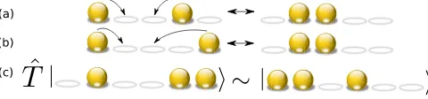
Because of this simple one-parameter labeling of the one-body states, anN-body interaction matrix element is labeled by2N indices. Additional constraints on its func-tional form arise when we consider interactions projected to a given Landau level (Fig.3). Because of the magnetic translation invariance, the interactions projected to a Landau level only allow for scattering that conserves total momentum or, equivalently, leaves the COM of the particles fixed. For example, the process in Fig. 3(a) is allowed, but the one in Fig.3(b)is forbidden. This special structure in the interaction Hamiltonian gives rise to the symmetry under many-body translations that shifts every particle byqorbitals at fillingν¼p=q[Fig.3(c)]. This is

FIG. 2. Boundary conditions considered in this paper, compat-ible with Landau gauge: cylinder (left diagram) and torus (right diagram). The associated single-particle statesψ_nðrÞ are arranged along a one-directional (1D) chain, with the parameter κ¼2πlB=Lycontrolling the distance between nearest-neighbor orbitals.

the symmetry that underlies the topological ground-state degeneracy.

The matrix elements of any interaction Vðr1;…;rNÞ

projected to a Landau level are given by

Vfnjg;fn0jg¼ Z

dr1;…; drN

×Y

j ψ

n0_jðrjÞψnjðrjÞ

Vðr1;…;rNÞ; ð9Þ

which corresponds to the second-quantized Hamiltonian

H¼X α

X

n

bαn†bαn;

bαn∝ X P

jnj¼n

pαðκn¯1;…;κn¯NÞe−

ðκ2_=2ÞPN j¼1n¯2j_c

n1;…; cnN:

ð10Þ

Here,n¯j¼nj−n=Ndenotes the orbital of particlejwith

respect to the COM, n¼n1þ þnN, and pα is a

polynomial in N variables κn¯j. The index α, as will be

clear from the explicit construction ofpα below, specifies the degree of the polynomial and, for a multicomponent state discussed in Sec.IV, its spin sector. The polynomial pα can be chosen to be real, as will be evident from its geometric construction later. From now on,nwill refer to the COM and not the index of a single particle previously appearing in Eq.(8).c†nj is the same operator as in Eq.(8),

creating thejth particle in statejn_ji. The Hamiltonian thus consists of a product sum over all positions of the COMn, as well as all polynomial degreesα.

Equations(9)and(10)represent a general translationally invariant Hamiltonian projected to a Landau level. This Hamiltonian has a rather special form: It decomposes into a linear combination of positive-definite operators bαn†bαn,

such that the form factor pαe−ðκ

2_=2ÞPN

j¼1n¯2j _{in each b}α n

depends only on the relative coordinates of particles. Any short-range Hamiltonian can be explicitly expressed in this form [34,35,44], which reveals its Laplacian structure.

Physically, Landau-level-projected Hamiltonians can be visualized as a long-range interacting 1D chain (Fig. 3). The interaction terms can be interpreted as long-range (though Gaussian-suppressed) hopping processes labeled byα. For eachα,Nparticles“hop”from sitesnjto sitesn0j,

j¼1;…; N according to a COM-independent amplitude given by pαðκn¯1;…;κn¯NÞe−

ðκ2_=2ÞPN

j¼1n¯2j_{, such that the}

initial and final COM n remains unchanged [Fig. 3(c)]. Note that although we use the term“hopping,”there is no clear distinction between hopping and“interaction”in our case, as opposed to the Hubbard model. Rather, hopping is designated for any interaction term that is purely quantum (i.e., not of Hartree form). The goal of the remainder of this

paper is to show how to systematically construct the polynomial amplitudes pα that need to be inserted into Eq. (10)to obtain the parent Hamiltonian for the desired quantum Hall state.

B. Geometric derivation

We now specialize Eq.(9)toN-body interactions that are Haldane PPs UN

m. One appealing feature of the

second-quantized form of Eq. (9) is that we can construct the desired PPs from symmetry principles alone, without referring to the first-quantized form of the interaction Vðr1;…;rNÞ.

The many-body PPs are, by definition, supposed to project onto orthogonal subspaces labeled bym, where, if applicable,mdenotes the relative angular momentum:

UN

m0UNm ¼ jψNm0ihψNm0jjψmNihψNmj ¼UmNδm0m: ð11Þ

This requires that

h0jbm0†

n bmnj0i∝ X

¯

n1þþn¯N¼0

pm0ðκn¯1;…;κn¯NÞ

×pmðκn¯1;…;κn¯NÞexp

−κ2XN

j¼1 ¯ n2_j

¼δm0m: ð12Þ

IfψN

mvanishes withmth total power asNparticles approach

each other, the polynomialpmmust be of degreem. Hence,

the PPs will becompletelydetermined once we find a set of polynomialsfp_mg such that (1) pm is of total degreem,

(2)pm has the correct symmetry property under exchange

of particles, i.e., is totally (anti)symmetric for bosonic (fermionic) particles, and (3) the pm’s are orthonormal

under the inner product measure

hpm0; pmi ¼ X

¯

n1þþn¯N¼0

pm0ðκn¯1;…;κn¯NÞ

×pmðκn¯1;…;κn¯NÞexp

−κ2XN

j¼1

¯ n2_j

: ð13Þ

Using the barycentric coordinates (Appendix A) to represent the tuple (n¯1;…;n¯N),

hpm0; pmi≈ Z

RN−1dWdΩpm

0ðW;ΩÞp_mðW;ΩÞ

× exp

−N−1

N W 2

JN−1ðW;ΩÞ

¼δm0m; ð14Þ

whereWandΩare the radial and angular coordinates of the vector ~x∈RN−1 _{representing the tuple (n¯}

JN−1is the Jacobian for the spherical coordinates inRN−1.

We have exploited the magnetic translation symmetry of the problem in quotienting out the COM coordinaten. (It is desirable to quotient outn¼PN

j njsincentakes values on

an infinite set when the particles lie on the 2D infinite plane, and that complicates the definition of the inner product measure.) Each quotient space is most elegantly represented as anN−1simplex in barycentric coordinates, where particle permutation symmetry (or subgroups of it) is manifest. Explicitly, the set of n¯j can be encoded in the

vector

~x¼κX

N

j¼1

¯

nj~βj; ð15Þ

where theNbasis vectorsfβ~_jgform a set that spansRN−1_.

A configuration (n¯1;…;n¯N) is uniquely represented by a

point~x∈RN−1_{that is independent ofn¼}PN

j nj. Since~x

should not favor any particular n¯j, any pair of vectors in

the basis fβ~_jgmust form the same angle with each other. Specifically,

~

βj·~βk¼

N N−1δjk−

1

N−1; ð16Þ

so that each vector points at the angle of π−cos−1ð1Þ= ðN−1Þ from another vector.

With this parametrization, the Gaussian factor reduces to the simple form

W2¼ j~xj2¼ N N−1κ

2XN

j¼1

¯

n2j: ð17Þ

Further mathematical details can be found in the examples that follow, as well as in AppendixA.

The integral approximation in Eq.(14)becomes exact in the infinite plane limit and is still very accurate for values of m where the characteristic interparticle separation is smaller than the smallest of the two linear dimensions of the QH system. In the following, we assume this to be the case; otherwise, there can be significant effects from the inter-action of a particle with its periodic images. This was systematically studied in the Appendix of Ref. [44] for N¼2. We note that the approximation in Eq. (14) does not affect the exact zero-mode property of the trial Hamiltonians constructed below.

C. Orthogonalization

We are now ready to evaluate the pseudopotentials. To find second-quantized PPs with relative angular momentum m, one needs to follow the rules listed in Table I. In the following, we shall execute this recipe explicitly for N¼2;3, and, to some extent, N ¼4-body interactions.

1. Two-body case

For two-body interactions, we have

hp_m0; p_mi ¼

Z _∞

−∞pm

0ðWÞp_mðWÞe−12W2_dW; ð18Þ

whereW ¼−2κn¯1¼2κn¯2. For thisN¼2case, we have allowedW to take negative values as the angular direction spans the 1D circle, which consists of just two points. The primitive polynomials for bosons aref1; W2; W4; W6;…g, while those for fermions arefW; W3; W5;…g. After per-forming the Gram-Schmidt orthogonalization procedure, the two-body PPs are found to beU2m∝κ3

P

nbmn†bmn, where

bm n ¼

X

¯

n1þn¯2¼0

pmðκn¯1;κn¯2Þe− 1

2κ2ðn¯21þn¯22Þ_cn=2þn¯

1cn=2þn¯2; ð19Þ

n=2þn¯j are integers, and pm is the mth-degree Hermite

polynomial given in TableII. In particular, we recover the Laughlin ν¼1=2 bosonic or ν¼1=3 fermionic state for m¼0orm¼1, respectively.

One can easily check that PPs become more delocalized inW space asm increases. Indeed,

κ2X

j

¯ n2j

¼1

2hW2i ¼ 1 2

Z _∞

−∞pmðWÞW 2_e−1

2W2_dW

¼mþ1

2; ð20Þ

which is reminiscent of the interpretation of m as the angular momentum of a pair of particles in rotationally invariant geometries (Fig.1). Obtaining the pseudopoten-tials in this second-quantized form is highly advantageous. In particular, note that this construction is free from ambiguities in the choice of Vðr₁;…;rNÞ since several

possible real-space interactions, e.g., those of the Trugman-Kivelson type [53], can all be grouped into the same m sector. This is discussed in more detail in AppendixB.

2. Three-body case

For N ¼3, the inner product measure takes the form

hpm0; pmi ¼ Z _∞

0 Z _2π

0 pm

0ðW;θÞp_mðW;θÞe−23W2_Wdθ_dW;

ð21Þ

TABLE I. Summary of the PP construction for spinless par-ticles. Examples of this procedure are given in Sec.V.

(1) Write down the allowed“primitive”polynomials[30,42,43] of degreem0≤mconsistent with the symmetry of the particles. (2) Orthogonalize this set of primitive polynomials according

with

¯

n1¼2W_3κ cosθ; ð22aÞ

¯ n2¼W_3κ

ffiffiffi

3 p

sinθ−cosθ

; ð22bÞ

¯ n3¼W_3κ

−pffiffiffi3sinθ−cosθ

: ð22cÞ

Each of the n¯j’s are treated on equal footing, as one

can easily check graphically. The above expressions are the simplest nontrivial cases of the general expres-sions for barycentric coordinates found in Eqs.(A3)–(A5) of Appendix A.

The bosonic primitive polynomials are made up of elementary symmetric polynomials S1; S2; S3 in the vari-ablesκn¯j¼κðnj−n=NÞ. SinceS1¼κ

P

jn¯j¼0, the only

two symmetric primitive polynomials are

−S2¼−κ2 X

i<j

¯ nin¯j¼

S21−2S2

2 ¼

κ2 2

X

i

¯ n2i ¼

1

3W2 ð23Þ

and

Y¼S3¼κ3 Y

i

¯ ni

¼κ3

27ð2n1−n2−n3Þð2n2−n3−n1Þð2n3−n1−n2Þ ¼ 2

27W3cos3θ: ð24Þ

The fermionic primitive polynomials are totally anti-symmetric and can always be written [42,43] as a symmetric polynomial multiplied by the Vandermonde determinant

A¼κ3ðn1−n2Þðn2−n3Þðn3−n1Þ ¼κ3_ðn¯

1−n¯2Þð¯n2−n¯3Þð¯n3−n¯1Þ

¼− 2

3pffiffiffi3W3sin3θ: ð25Þ

Note thatW2is of degree 2, whileAandYare of degree 3. All of them are independent of the COM coordinate n, as they should be. N¼3 PPs were derived in Ref. [44] through explicit integration, and the approach discussed here considerably simplifies those computations by exploit-ing symmetry.

To generate the fermionic (bosonic) PPs up to U3m,

we need to orthogonalize the basis consisting of all possible (anti)symmetric primitive polynomials up to degree m. For instance, the first seven (up to m¼9) three-body fermionic PPs are generated from the primi-tive basis fA; AW2; AY; AW4; AYW2; AY2; AW3g. Note that the last two basis elements both contribute to the m¼9 PP sector.

The three-body PPs are found to beU3m∝κ3 P

nbmn†bmn,

where

bm n ¼

X

n1þn2þn3¼n

pmðW; Y; AÞe− 1 3W2_cn

1cn2cn3; ð26Þ

with the polynomialspm listed in TableIII. These results

are fully compatible with those from Ref. [42]. As mentioned, there can be more than one (anti)symmetric polynomial of the same degree for sufficiently largem. This leads to the degenerate PP subspace, a specific example of which is presented in Sec.VA 2.

3. N≥4-body case

For general PPs involving N bodies, the inner product measure takes the form

TABLE II. Representative polynomials pm for the first few N¼2-body PPs for bosons and fermions.

pmðWÞe−W 2₌₄

represents the probability amplitude that two particlesW=κsites apart along a chain are involved in a two-body hopping.

m BosonicpmðWÞ FermionicpmðWÞ

0 1 0

1 0 W

2 _ð1=pffiffiffiffi_{2!Þð−1þW}2_Þ 0

3 0 _ð1=pffiffiffiffi_{3!Þð−3þW}2_ÞW

4 _ð1=pffiffiffiffi_4!Þð3−6W2_þW4_Þ 0

5 0 _ð1=pffiffiffiffi_{5!Þð15−10W}2_þW4_ÞW

6 _ð1=pffiffiffiffi_{6!Þð−15þ45W}2_−15W4_þW6_Þ 0

hpm0; pmi ¼ Z _∞

0 e −N−1

NW2WN−2dW

× Z _2π

0 dϕN−2 Y N−3

k¼1 Z _π

0 sin

N−2−k_ðϕ kÞdϕk

×pm0ðW;ϕ1;…;ϕN−2ÞpmðW;ϕ1;…;ϕN−2Þ;

ð27Þ

where the Jacobian determinant from Eq. (14) has already been explicitly included. One transforms the tuple fn¯1;…;n¯Nginto (N−1)-dim spherical coordinates via the

barycentric coordinates detailed in AppendixA.

The bosonic primitive basis is spanned by the elementary symmetric polynomials fS₂; S3;…; SNg ¼

fP_ijn¯in¯j; P

ijkn¯in¯jn¯k;…; Q

jn¯jg and combinations

thereof. For instance, with N¼5 particles at degree m¼6, there are three possible primitive polynomials: S3₂; S2₃, andS2S4. The fermionic primitive basis is spanned by all the symmetric polynomials as above, times the degree ðN

2Þ Vandermonde determinant Q

i<jðn¯i−n¯jÞ

shown in Fig. 4.

From the examples above, one easily deduces the degeneracy of the PPs UNm to be Pðm; NÞ−Pðm−1; NÞ

for bosons and Pðm−ðN₂Þ; NÞ−Pðm−1−ðN₂Þ; NÞ for fermions, where Pðm; NÞ is the number of partitions of the integer N into at most m parts [42,43]. In particular, the degeneracy is always nontrivial (≥2) wheneverN ≥4 andm≥4.

IV. GEOMETRIC CONSTRUCTION OF PSEUDOPOTENTIALS: SPINFUL CASE

In the presence of“internal degrees of freedom”(DOFs) which we also refer to as “spins” or “components” for simplicity, there are considerably more possibilities for the diverse forms of the PPs. This is because the PPs consist of products of spatial and spin parts, and either part can have

TABLE III. The polynomialspmforN¼3-body PPs for bosons and fermions up tom¼9. Note that there is more than one possible PP for largermsince there are multiple ways to build a homogeneous (anti)symmetric polynomial from the primitive and elementary symmetric polynomials. For instance, withYandAdefined in Eqs.(24)and(25), there are two possible bosonic PPs form¼6since there are two ways (W6 and Y2) to build a homogeneous 6-degree polynomial from elementary symmetric polynomials. For the fermionic cases, we have explicitly kept only one factor ofAsince even powers ofAcan be expressed in terms ofW2andY. For all cases, the mean-square spread of the PPs also increases linearly withm, i.e.,κ2hP3_jn¯2ji ¼mþ1[compare with the two-body case in Eq.(20)].

m BosonicpmðW; YÞ FermionicpmðW; Y; AÞ

0 1 0

1 0 0

2 1−2_3W2 0

3 ₃pffiffiffi_2Y A

4 1−4_3W2þ2_9W4 0

5 pffiffiffi_2Yð6−W2_{Þ Að2−}1

3W2Þ

6 (i)1−2W2þ2₃W4−₈₁4W6 (ii)₈₁1

ffiffi 2 5 q

ð2W6−729Y2Þ ð3=pffiffiffi5ÞAY

7 _ð2=3pffiffiffi_{5Þð45−15W}2_þW4_ÞY pffiffiffiffiffi_10Að1−1

3W2þ451W4Þ

8 (i)1þ₂₄₃2 W2ðW2−6Þð54−18W2þW4Þ

(ii)₂₄₃1

ffiffiffiffi 2 35 q

ð2W2−21Þð2W6−729Y2Þ

3 ffiffi7 5 q

ð1− 2 21W2ÞAY

9 (i)

ffiffiffiffiffiffi 6 155 q

Yð−30þ15W2−2W4þ18Y2Þ

(ii)₂₇1

ffiffiffiffiffiffiffi 2 1085 q

Yð−5760W2þ756W4−31W6þ81ð140þ9Y2ÞÞ

(i)ðA=pffiffiffi5Þð−10þ5W2−2₃W4þ₈₁2W6Þ

(ii)ðA=81pffiffiffiffiffiffiffiffi105ÞðW6−729Y2Þ

FIG. 4. The primitive polynomials have beautiful geometric shapes when plotted inN−1-dim spherical coordinates. Shown above are the constantW plots of the antisymmetric polynomial

A¼ ðn¯1−n¯2Þðn¯1−n¯3Þðn¯1−n¯4Þðn¯2−n¯3Þðn¯2−n¯4Þðn¯3−n¯4Þ (left

diagram) and the degree m¼4 symmetric expression in the orthonormalized space spanned by the elementary symmetric polynomials 1; S2; S3; S4, and S22 (right diagram). On the left,

many possible symmetry types, as long as they conspire to produce an overall (anti)symmetric PP in the case of (fermions) bosons.

A generic multicomponent PP takes the form

UN m ¼

X

λ X

σ UN

m;λjσλihσλj: ð28Þ

The notation here requires some explanation. λ¼ ½λ1;λ2;… defines a partition of all particles into several subgroups λ_i, each of which imposes a symmetry con-straint among particles of this subgroup. Associated with this partition, or symmetry type, isUN

m;λ, which is anmth

order spatial term [in ðn¯1;…;n¯NÞ space] exhibiting this

symmetry. jσλi ¼ jσ₁σ₂…i refers to an (internal) spin basis that is consistent with the symmetry type λ. Each symmetry type corresponds to a partition of N, with P

jλj¼N. For N bosons, λ represents the situation

where there is permutation symmetry among the first

λ1 particles and the next λ2 particles, etc., but no additional symmetry between the λ_i subsets. This is often represented by the Young tableau with λ_i boxes in the ith row. For fermions, we use the conjugate representation λ¯, with the rows replaced by columns and symmetry conditions replaced by antisymmetry ones. For instance, the totally (anti)symmetric types are ½1;1;…;1 and ½N, respectively.

Hence, the space of PPs is specified by three parameters: N, the number of particles interacting with each other;m, the total relative angular momentum or the total polynomial degree in n¯i; and b, the number of internal DOFs (spin).

While the symmetry typeλ, and henceUNm;λ, depends only on

Nandm, the set of possiblejσλialso depends onb. To further illustrate our notation, we specifyN; m; bparameters for the interactions relevant to some commonly known states: In the archetypical single-layer FQH states, we have b¼1 com-ponents, and theN ¼2PP interactions for the Laughlin state penalize pairs of particles with relative angular momentum m, whereν¼1=ðmþ2Þis the filling fraction. For bilayer FQH states, we have b¼2 and N¼2-body interactions. PPs as energy penalties in the [2] sector with angular momentum< mand [1,1] sectors with angular momentum < n give rise to the HalperinðmmnÞ states. Here, the [2] sector is also known as the triplet channel, as it is spanned by the following three basis vectors: fj↑↑i;j↑↓iþ j↓↑i;j↓↓ig. By contrast, the [1,1] sector only contains fj↑↓i−j↓↑ig, as dictated by antisymmetry.

A. Multicomponent pseudopotentials for a given symmetry

The construction of multicomponent PPs here parallels that of multicomponent wave functions described in Ref. [43]. For completeness, we first review this con-struction and proceed to show how an orthonormal

multicomponent PP basis, adapted to the cylinder or torus, can be explicitly found through the geometric approach. We describe how to first find the spatial part of the PP UN

m;λ, and second the spin basis jσλi.

1. Spatial part

For each symmetry type λ, we can construct the spatial part UN

m;λ with elementary symmetric polynomials in

subsets of the particle indices n¯i¼ni−n=N. They are,

for instance, S1;12¼n¯1þn¯2, S2;234¼n¯2n¯3þn¯3n¯4þ ¯

n2n¯4, etc. Of course, we must haveS1;123…N¼ P

in¯i¼0.

Like in the single-component case, the spatial partUNm;λ

consists of a primitive polynomial that enforces the sym-metry and a totally symmetric factor that does not change the symmetry. Here, the main step in the multicomponent generalization is thereplacementof primitive polynomials 1 and A by primitive polynomials consistent with the symmetry type λ. As the simplest example, the primitive polynomial inUN¼3

m¼1;½2;1 isS1;12 ¼−n¯3(and

cyclic permutations). It is the only possible degreem¼1 expression symmetric in two (but not all three) of the indices. In general, there can be more than one candidate monomial obeying a symmetry consistent with λ. For instance, for UN_m¼¼32;½2;1they areS21;12¼ ð¯n1þn¯2Þ2andS2;12¼n¯1n¯2(and

cyclic permutations thereof). To find the primitive poly-nomials, we have to construct one or more linear combinations of these terms, which do not have any higher symmetry other than [2,1] (i.e., in this case, this higher-symmetry channel could be [3]). Elementary com-putation reveals that the only primitive polynomial should beS2_1;12þ2S2;12 because it is the only linear combination

that is manifestly symmetric in indices 1,2anddisappears upon symmetrization over all three particles.

N¼4, m¼2, λ¼ ½2;2.—As a more involved example, we demonstrate how to find the primitive polynomial corresponding to the symmetry type [2,2]. Independent monomials that satisfy this symmetry includeS21;12,S2;12,

andS2;34. The primitive polynomial is then given by the

linear combination

S2_1;12þμ1S2;12þμ2S2;34; ð29Þ

with μ₁ and μ₂ to be determined by demanding that the linear combination disappears upon symmetrizing over permutations under [3,1] and [4]. The symmetrized sums are

2½ðn2þn3Þ2þ ðn2þn4Þ2þ ðn3þn4Þ2

þμ1ðn1n2þn1n3þn2n3Þ þμ2ðn1n4þn2n4þn3n4Þ ð30Þ

4ðn2

2þn23þn24þn2n3þn3n4þn2n4Þð4−μ1−μ2Þ: ð31Þ

Setting them both to zero, we find μ₁¼μ₂¼2, so the primitive polynomial isS21;12þ2S2;12þ2S2;34.

N¼3,m¼2,λ¼ ½2;1.—The above procedure works for arbitrarily complicated cases but quickly becomes cum-bersome. This is when our geometric approach again becomes useful. We first write down the relevant mono-mials in barycentric coordinates given by Eq. (22) for N¼3bodies [or Eq.(A12)for generalN]. The coefficients in the primitive polynomial can then be elegantly deter-mined through graphical inspection. We demonstrate this explicitly by revisiting the example on λ¼ ½2;1. Recall that the primitive polynomial (call itβ_m¼2≡β₂) is a linear combination of S21;12 andS2;12, i.e.,

β2¼S21;12þμS2;12

¼−W2

9κ ðμ−2þ ð1þμÞðcos2θ−

ffiffiffi

3 p

sin2θÞÞ; ð32Þ

whereθ¼0;2π=3;4π=3points towards the vertices favor-ingn¯1;n¯2;n¯3, respectively. The correct value ofμwill cause

β2to disappear under symmetrization of the three particles. Graphically, this means that the lobes of three copies of the plot ofβ₂, each rotated an angle2π=3from each other, must cancel upon addition. This is illustrated in Fig. 5, where

μ¼2is readily identified as the correct value.

All in all, we have the m¼2 primitive polynomial for [2,1]:

β2¼ ð¯n3Þ2þ2¯n1n¯2¼W 2

3 ð−cos2θþ

ffiffiffi

3 p

sin2θÞ: ð33Þ

N¼3, m¼1, λ¼ ½2;1.—The reader is invited to also visualize the simpler case for the [2,1] sector, which takes the form

β1¼S1;12¼−n¯3¼₃W_κðcosθþ ffiffiffi

3 p

sinθÞ: ð34Þ

Compared to the antisymmetric case for fermions, we have two primitive polynomials β₁;β2, instead of just A. The primitive polynomials for a wide variety of cases are also listed in Tables II and III of Ref.[43], and can alternatively be systematically derived via the theory of Matric units explained in the appendix of the same reference.

2. Admissible spin bases

In general, not all possibleN-particle spin bases survive under symmetrization with respect to a given symmetry typeλ. Only those that survive should be included, i.e., are admissible, in the set of basis injσλi. For instance, the basis

jαααi does not appear in jσ½2;1_{i. To see this, try}

sym-metrizing the combination pðn¯1;n¯2;n¯3Þjαααi subject to the condition that pðn¯1;n¯2;n¯3Þ has no higher sym-metry than λ¼ ½2;1, i.e., the totally symmetrized sum S½pðn¯1;n¯2;n¯3Þ ¼0. Obviously, pð¯n1;n¯2;n¯3Þjαααi then has to symmetrize to zero and should not be included in [2,1].

We can write down the set of admissible bases by looking at the labelings of semistandard Young tableaux. From Ref. [43], the admissible bases in jσλi, up to permutations, are in one-to-one correspondence with the labelings of semistandard Young tableaux with numbers 1 to N. (A semistandard Young tableau has nondecreasing entries along each row and strictly increasing entries along each column.) For instance, a symmetry type of [3,1] with b¼3corresponds to labelings (with labelsa; b; c defined to be in increasing order):

½aaa; b;½aab; b;½aac; b;½abb; b;½abc; b; ½acc; b;½aaa; c;½aab; c;½aac; c;½abb; c;

½abc; c;½acc; c;½bbb; c;½bbc; c;½bcc; c and ½ccc; c;

where rows are separated by commas. From these, the admissible states for λ¼ ½3;1 can be written down by copying the labelings verbatim:

jaaabi;jaabbi;jaacbi;jabbbi;jabcbi; jaccbi;jaaaci;jaabci;jaacci;jabbci;

jabcci;jaccci;jbbbci;jbbcci;jbccci; and jcccci: 0.6 0.4 0.2 0.2 0.4 0.6

0.6 0.4 0.2 0.2 0.4 0.6

FIG. 5. Polar plots ofβ₂ðθÞ as a function ofθ, with μ¼0.5 (blue curve) andμ¼2(purple curve).β₂ðθÞ þβ₂ðθþ2π=3Þ þ

β2ðθþ4π=3Þis zero only when the lobes are of equal size, which

In the Young tableau corresponding to λ, each row represents a set of particles that are symmetric with each other in the λ representation. The requirement that labels increase monotonically within each row defines an ordering and prevents the repeated listing of basis states related by permutation. The requirement of strictly increasing label-ings down each column also prevents this and also avoids the listing of bases that do not survive under symmetry constraints.

With these preliminary considerations, we are now in a position to formulate the general recipe for constructing PPs in the multicomponent case, which is given in TableIV. In the following section, we apply this recipe to the case of SU(2) spins with three-body interactions.

B. Example: N¼3-body case for SU(2) spins

Here, we explicitly work out the multicomponent case b¼2, which is also the most common multicomponent scenario. We focus onN¼3-body interactions to illustrate the nontrivial aspects of our approach.

The symmetry type is given by ½λ₁;λ2 ¼ ½N=2þS; N=2−S, where S is the total spin of the particles. Let us denote the spins by ↑;↓. There are only N¼3 boxes in the Young tableaux, with the following possible symmetry types: [3], [2,1], [1,1,1].

For type λ¼ ½3, the possible spin bases are j↑↑↑i, j↑↑↓i,j↑↓↓i, andj↓↓↓i. Forλ¼ ½2;1, the possible spin bases arej↑↓↓i,j↑↑↓i, corresponding to tableau labelings ½↑↓;↓and½↑↑;↓, respectively. Forλ¼ ½1;1;1, there is actually no admissible spin basis: Total (internal DOF) antisymmetry is impossible for three particles, if there are only two different spin states to choose from.

Consider bosonic particles in the following. The sym-metry type [3] case corresponds to the primitive polynomial 1, so the resultant PP takes the same form as in the single-component case. After symmetrizing the spin part, we have the following available sets of spin channels for [3]:

fj↑↑↑ig;

fj↑↑↓i;j↑↓↑i;j↓↑↑ig; fj↓↓↑i;j↓↑↓i;j↑↓↓ig; fj↓↓↓ig:

For the PPU3_m;½3∝κ3

P

nbmn†bmn, we have

bmn†j0i ¼ X P

jnj¼n

pme− 1

3W2j↑↑↑i ð35Þ

forS¼3=2, and

b†nmj0i ¼S 2 6

4_PX

jnj¼n

pme− 1

3W2j↑↑↓i

3 7

5 ð36Þ

for S¼1=2. Other contributions with S→−S can be obtained via the identificationj↑i↔j↓i. Here,j↑↑↓iis the shorthand forc†_n1↑c†_n2↑c_n†_3↓j0i, etc., and pm≡pm;½3 refers

to thesamepolynomial as in the single-component case. To construct the orthonormal PP basis for the first fewm, we orthogonalize the set fβ₁;β2;β1W2;β2W2;β1Y;β2Y;

β1W4;…g. The results are shown in TableV. Notice that the first PP for symmetry type [2,1] occurs at m¼1, whereas that of single-component bosons or fermions occurs at m¼0 and m¼3, respectively. Indeed, there are more ways of constructing PP polynomials when only a subgroup of the full symmetric or alternating group is involved. The onset of PPs degenerate in m also occurs earlier, atm¼4.

TABLE IV. Summary of the PP construction procedure for the multicomponent case. Examples of this procedure are given in Sec.V.

(1) GivenN,m, andb, specify which symmetry type the PP is associated with. For example, we specify the [2] or the [1,1] channel when computing PPs realizing the fermionic Halperin states in bilayer QH systems (b¼2; N¼2).

(2) Next, determine the appropriate primitive polynomials by finding the coefficients multiplying the allowed monomials. Then, multiply the primitive polynomial by symmetric polynomials and orthogonalize to obtain the spatial partsUN

m;λ. (3) Finally, choose the desired admissible spin channels and

(anti)symmetrize the resultant product of the spatial and spin parts depending on whether we want a bosonic or fermionic PP.

TABLE V. The polynomials pm for the first fewN¼3-body PPs for bosons in the total spinjSj ¼1₂, i.e.,λ¼ ½2;1channel. The primitive polynomialsβ₁andβ₂are given by Eqs.(33)and (34). The cos4θ;sin4θ;cos5θ;sin5θ can all be decomposed into the elementary symmetric polynomials and primitive poly-nomialsW; Y;β1, andβ2.

m pm;½2;1ðβ1;β2; W; YÞ

1 β₁

2 ð1=pffiffiffi3Þβ2

3 1

3 ffiffiffi

2

p

β1ð−3þW2Þ

4(i) ð1=pffiffiffi5Þðβ2þ6β1YÞ

4(ii) ð1=27pffiffiffi5Þ½−54β2þ12β2W2þW4ðcos½4θ þpffiffiffi3sin½4θÞ

5(i) ð1=pffiffiffiffiffi33Þ½β1ð−3þ2W2Þ þ6β2Y

5(ii) 1 81

ffiffiffiffi 2 55 q

To illustrate the full procedure for PP construction with internal DOFs, we detail the case ofS¼−1=2below. For m¼1,

b1n†j0i ¼S 2 6

4_PX

jnj¼n

ð−n¯3Þe−13W2j↑↓↓i

3 7 5

¼−e−1

3W2½ð_n¯₂þ_n¯₃Þj↑↓↓i

þ ð¯n1þn¯3Þj↓↑↓i þ ðn¯1þn¯2Þj↓↓↑i

¼e−13W2½_n¯₁j↑↓↓i þ_n¯₂j↓↑↓i þ_n¯₃j↓↓↑i_; ð₃₇Þ

while for m¼2, we have

b2n†j0i ¼S 2 6

4_PX

jnj¼n

ðð¯n3Þ2þ2¯n1n¯2Þe−13W2j↑↓↓i

3 7 5

¼e−13W2½ðð_n¯₂Þ2þ ð_n¯₃Þ2þ2¯_n1ð¯_n2þ_n¯₃ÞÞj↑↓↓i

þ ðð¯n1Þ2þ ð¯n2Þ2þ2¯n3ðn¯1þn¯2ÞÞj↓↓↑i

þ ðð¯n1Þ2þ ð¯n3Þ2þ2¯n2ðn¯1þn¯3ÞÞj↓↑↓i: ð38Þ

Expressions forS¼1=2 are obtained viaj↑i↔j↓i. For the present case of SU(2) spins, i.e., b¼2, there exists a nice closed-form generating function for the dimension of the spatial basis for each m. Define the generating functionZ½λ1;λ2ðqÞ¼

P

mdð½λ1;λ2;mÞqm, where

dð½λ1;λ2;mÞis the number of different polynomials with degreemand symmetry type½λ₁;λ2. It can be shown that for bosons,

Z½λ1;λ2ðqÞ ¼

1−q

Qλ1

m¼1ð1−qmÞ Qλ2

n¼1ð1−qnÞ

−Q_λ1þ1 1−q

m¼1ð1−qmÞ Q_λ2−1

n¼1ð1−qnÞ

: ð39Þ

This result is obtained[43]by considering the dimension-ality from two symmetry subsets and then subtracting overlaps from the higher-symmetry case ½λ₁þ1;λ₂−1. The dimension is related to theq-binomial coefficient. For b >2, however, the situation is much more complicated, involving Kostka coefficients that count the number of semisimple labelings ofλ with a given alphabet.

V. PSEUDOPOTENTIAL HAMILTONIANS: CASE STUDIES

In this section, we provide several applications of the general pseudopotential construction developed in the previous sections, with examples arranged in the order of increasing complexity. We start with spin-polarized states (Sec.VA), whose Hamiltonians have been obtained via alternative methods and are well known in the literature.

As an illustration of the method, we provide a detailed derivation of the fermionic Gaffnian parent Hamiltonian. Note that the resulting second-quantized form of the Hamiltonian applies (with minimal modifications) to both cylinder and torus geometries. In addition to pedagogical examples that illustrate our approach, we construct pseudopotential Hamiltonians for some non-Abelian states that have not been available in the literature for any geometry.

The main sequence of steps is stated as follows: (i) Assuming that the ground-state wave function is known in the first-quantized form, find its thin-torus pattern (this step has been frequently discussed in the literature; for completeness, we provide a brief summary in AppendixC). (ii) Using the formalism developed in the previous sections, write down the parent Hamiltonian corresponding to the root pattern in the second-quantized form. (iii) Use numerics (exact diagonalization) to verify that the ground state of the proposed Hamiltonian is indeed given by the initial wave function. The verification criteria include testing for the unique zero-energy ground state at the given filling factor, the correct thin-cylinder root patterns as the circumference of the cylinder is taken to zero, and the level counting of entanglement spectra. For the purpose of numerical calculations, we place a finite total number of particlesN on the surface of a torus or an open cylinder. The two linear dimensions of the Hall surface (LandH) satisfy the relation LH¼2πl2BNorb, where Norb is the

number of available orbitals (it is equal to Nϕ on the torus and equal toNϕþ1 on the cylinder). Unless stated otherwise, we also assumeL¼H.

A. Spin-polarized states

The construction of two-body as well as the shortest-range three-body pseudopotential Hamiltonians has been discussed in depth in the literature (see, e.g., Refs.[4,9– 11]). Starting from there, as our most elementary example for spin-polarized particles, we consider ground states of longer-ranged three-body potentials: the fermionic Gaffnian state at filling ν¼2=5 as well as the Haffnian and the generalized Moore-Read Pfaffian state at filling

ν¼1=q, for which the q¼4 case will be discussed in detail.

1. Fermionic Gaffnian

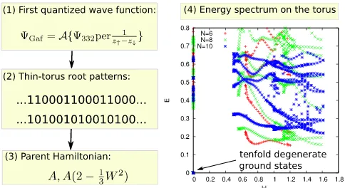
The derivation of the fermionic Gaffnian parent Hamiltonian is summarized in Fig.6. The wave function of the Gaffnian state on the infinite plane is given by[54]

ΨGaf ¼A Ψ332ðfz↑g;fz↓gÞPer

1 z↑−z↓

; ð40Þ

state, the above wave function reflects the underlying“ two-component”nature of the Gaffnian state: In order to write down the wave function, we have divided electrons into two groups,↑and ↓(not to be confused with physical spin), that are correlated through the Jastrow factors within the 332 Halperin state, which is defined as

Ψ332ðfz↑; z↓gÞ ¼ Y

i<j

ðz↑;i−z↑;jÞ3 Y

i<j

ðz↓;i−z↓;jÞ3

×Y

i;j

ðz↑;i−z↓;jÞ2; ð41Þ

as well as the “permanent"

Per

1 z↑−z↓

¼X σ

1

Q

jðz↑j−z↓σðjÞÞ

: ð42Þ

Ultimately, the distinction between ↑ and ↓ particles is erased by the overall antisymmetrization A, producing a well-defined single-component wave function.

Having obtained the first quantized wave function for the Gaffnian, the second step is to determine its thin cylinder root patterns. (Note that a similar but different analysis can also be executed on the sphere by analyzing the root partitions of the parent Hamiltonian null space[55]). The detailed procedure for finding the root patterns of Halperin bilayer states was given in Ref. [56], of which a brief summary is outlined in Appendix C. The Gaffnian wave function vanishes as power 6 as three particles are brought

together; hence, its thin-torus root patterns are 1100011000…and1010010100…, accordingly.

From the form of the root patterns, we conclude that we needUN¼3

m¼3 and UNm¼¼35 terms in order to build the parent

Hamiltonian. The polynomial amplitudes for these terms can be found in Eq.(26)and TableIII. The Gaffnian parent Hamiltonian therefore reads

H¼X

n

b†nbnþγ X

n

d†ndn; ð43Þ

bn¼ X

¯

n1þn¯2þn¯3¼0

Aðn¯1;n¯2;n¯3Þe−ðκ

2_=2ÞP3 j¼1n¯2j_c

n1cn2cn3; ð44Þ

dn¼ X

¯

n1þn¯2þn¯3¼0

Aðn¯1;n¯2;n¯3Þ

2−1

3W2ðn¯1;n¯2;n¯3Þ

×e−ðκ2=2Þ

P₃ j¼1n¯2j_c

n1cn2cn3; ð45Þ

where as before n¯j¼nj−n=3. The Hamiltonian (43)

assigns positive energies tom¼3;5 in a cluster of three particles in an infinite system, while all the other energies are exactly zero. The constantγ tunes the ratio of the two nonzero energies and can be set to any positive number. The precise value ofγdoes not affect the ground-state wave function or its energy, but it does have an effect on the energetics of the low-lying excited states. In the following, for the sake of brevity, we refer to the Hamiltonian in Eq.(43) simply byAþγAð2−1₃W2Þ.

Finally, having obtained the parent Hamiltonian, we can verify that it yields the correct ground state we started from [Eq.(40)]. As we see in Fig.6, exact diagonalization on the torus forN ¼6;8;10electrons consistently finds a zero-energy ground state that is tenfold degenerate and has zero momentum (i.e., does not break translation symmetry). One can further verify that we have obtained the correct ground state by computing its entanglement properties, as we discuss below. Another nontrivial check is to perform diagonalization on a torus stretched along one axis and directly identify the root patterns in the thin-torus limit. In doing so, we find, as expected, the ground states to evolve to the single Fock states1100011000…and1010010100… (and those obtained from these by COM translation), in agreement with the fermionic Gaffnian state.

2. Pfaffians and Haffnians

We next consider the generalized non-Abelian Pfaffian state at 1=q filling[8,11]. The wave function in the disk geometry reads

Pf

1 zi−zj

Y

i<j

ðzi−zjÞq; ð46Þ

where even (odd)qcorresponds to a fermionic (bosonic) state. The Pfaffian is defined as

PfðAÞ ¼ 1 2n=2_ðn=2Þ!

X

σ∈Sn

sgnðσÞY

n=2

i¼1

Aσð2i−1Þ;σð2iÞ;

where A is the n×n skew-symmetric matrix Aij¼1=

ðz_i−zjÞforneven. The caseq¼2reduces to the familiar

Moore-Read state, which is the ground state of the purely three-body interaction U3₃. One would naively expect that q >2states can be obtained by adding two-body terms to U33, but as one can explicitly verify, this is not the case.

By a power-counting procedure[11](further elaborated on in Appendix C), the root configuration of the 1=q -Pfaffian state is given by

10q−2₁₀q₁₀q−2₁₀q_……10q−2₁₀q_{…; ð47Þ}

where0q represents a string ofqzeros. It follows that its parent Hamiltonian is given by the three-body PP

U3_m¼3ðq−1Þ; ð48Þ

as well as all nonzero spinless two-body PPs

U2m<q−2: ð49Þ

For the more interestingq¼4case that we have studied numerically, we require the two-body U2₁ PP and three-bodyU3_9;ðiÞandU39;ðiiÞPPs given by Eq.(26)and TableIII.

[Again, we emphasize that U’s promoted to how they appear in the Hamiltonian should be understood as poly-nomial amplitudes that enter the definition of operators b†n; bn in Eq.(10).]

Note that labels (i),(ii) stand for two linearly independent three-body PPs that occur form¼9. Thus, the1=4Pfaffian state is an example whose parent Hamiltonian contains a degenerate subspace of PPs. The state can alternatively be obtained numerically through Jack polynomials [57] and the root configuration given above. We have confirmed that the overlap between the ground state of the parent Hamiltonian and the Jack polynomial wave function is equal to 1 (within machine precision) for q¼4andN¼ 6;8 electrons. Note that experiments [58] find some evidence for an incompressible, potentially non-Abelian,

ν¼1=4 state. This may be attributed to the Pfaffian1=4 state, although theoretical calculations suggest that the Halperin 553 state is also a candidate [59].

For our final spin-polarized example, we consider the fermionic Haffnian state [60], whose bosonic counterpart was recently considered in Ref. [39]. The fermionic Haffnian occurs at the filling fraction ν¼1=3, and, up to COM translation, has the following root patterns[61]on the sphere: 110000110000… and 100100100100… The latter pattern is identical to that of the Laughlin state. The fermionic Haffnian vanishes as power 7 as three particles are brought together; hence, we need to impose an energy

penalty for m¼6 too, and the parent Hamiltonian consists of

U3₃; U3₅; and U3₆; ð50Þ

which are given by Eq.(26)and Table III.

B. Spinful states

We have previously mentioned that if we allow the spin degree of freedom to enter, the number of possible states obviously becomes much richer with interactions involving three or more particles. A systematic investigation of these states is left for future work. Here, we content ourselves with illustrating our method by formulating parent Hamiltonians for several states that have been the subject of recent attention: the spinful Gaffnian[62]and the NASS states [63]. The Hamiltonians for these states have pre-viously been written down for the sphere (or disk) geometry, which we now extend to the cylinder and torus. Furthermore, we propose the parent Hamiltonian for a certain type of state involving the permanent state (“221 times permanent” state [64]), for which the Hamiltonian was previously unknown.

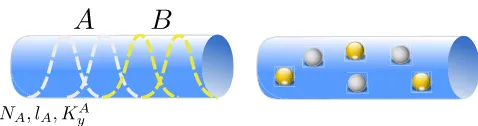
In addition to formulating the parent Hamiltonians, we also computed the orbital entanglement spectrum (OES) and the particle entanglement spectrum (PES) for the respective states. Figure 7 illustrates the two types of partitioning in the case of an open cylinder. After perform-ing the cut, the entanglement spectrum can still have some remaining symmetry that can be used to classify the Schmidt levels. For example, for the OES, the total number of particlesNA and the total number of orbitalslA

in the left subsystem remain good quantum numbers. On the other hand, for the PES, the translation or rotation symmetry of the full system is preserved. For an open cylinder, as in Fig.7, this means that the total momentum KAy of the left subsystem is also a good quantum number:

FIG. 7. Two choices of partitioning the system for computing the entanglement spectrum. The orbital cut (left diagram) amounts to partitioning the system into two groups of orbitals

AandB, and tracing out the orbitals inB(marked yellow). The Schmidt levels ofAcan be classified by the number of particles

KAy ¼ X

m∈A

mnˆm; ð51Þ

with nˆm the density operator acting on the momentum

orbital m. This linear momentum on the cylinder corre-sponds to theLz projection of angular momentum on the

sphere. The PES on the sphere, however, is also invariant under full SU(2) rotation; i.e., it forms multiplets of L2. This symmetry is absent on a cylinder, where we can only use KA

y to classify the levels of the entanglement

spectrum. This is discussed in more detail in the example in Sec. V B 1. As we perform an orbital partition, the symmetry of the subsystem is reduced, and even on the sphere, the only remaining quantum number is Lz. Thus,

the OES on the sphere can be directly compared with the OES on the open cylinder. Finally, for spinful states, the spin quantum number commutes with the reduced density operator of the OES and thus allows for additional resolution of the ES level counting [65].

1. Spin-singlet Gaffnian state

The spin-singlet Gaffnian state is a nontrivial spinful generalization of the bosonic spin-polarized Gaffnian state by Davenport et al. [62]. In addition to the two spin-polarized three-body terms with S¼3=2, its parent Hamiltonian also contains the shortest-range (m¼1) term withS¼1=2. In total, this encompasses the PPs

U3_0;S¼3=2; U32;S¼3=2 and U31;S¼1=2: ð52Þ

As such, the spin-singlet Gaffnian wave function vanishes as the third power in theS¼3=2channel and the second power inS¼1=2. These projectors are given by Eqs.(26) and(35)and TableIIIforU3_0;3=2andU3_2;3=2, and Eq.(37)for U3_1;S¼1=2(with both spin orientationsj↑i↔j↓i). In addition

to these, we also add the total spin operator S2 to our Hamiltonian, to ensure that the ground state is a spin singlet.

By diagonalizing the Hamiltonian(52)numerically, we find a zero-energy ground state at filling factor ν¼4=5 and shift of −3 on a finite cylinder for N¼4;8, and 12 particles. We have furthermore computed the PES [27] for N¼12particles and Nϕ¼12 flux quanta, shown in Fig. 8. As illustrated in Fig. 7 (right), to perform a PES “partition,” we divide the system into parts A and B, which both contain Nϕorbitals, butNA andNB particles,

respectively, such that NAþNB¼N. To obtain Fig. 8,

we have traced outNB ¼6particles from the system. The

PES obtained in this way provides information about the counting of quasihole excitations of the given state, as shown in Ref. [27].

We compare the counting in Fig.8with the correspond-ing PES obtained on the sphere in Davenport et al. [62]. Note that our result in Fig. 8superficially looks different

from the result in Ref. [62]. This is because the PES partition preserves the symmetry of the ground state, causing the PES on the sphere to have exact rotational symmetry, which is absent for our open cylinder. In other words, on an open cylinder, the good quantum number after partitioning is only the linear momentumKA

y. This quantum

number, in turn, corresponds to theLzprojection of angular

momentum on the sphere. This, however, does not exhaust all symmetries of the PES on the sphere, where the full angular momentum L2 is a good quantum number. This additional degeneracy of the PES is factored out in Ref. [62]. Furthermore, on both the sphere and cylinder, because of the singlet property of the wave function, we expect the PES levels to be multiplets of the S2 operator [65], as can be verified in Fig. 8. The most important universal information is the counting of PES levels per momentum sector, which we find to be in agreement with Ref.[62]. As we restore theL2degeneracy in the PES given in Ref. [62], the counting for the first three sectors is a single level withS¼1andLz_{¼22, four levels atL}

z¼21

(two with S¼1 and two with S¼0), and ten levels at Lz¼20(one of them withS¼2, six withS¼1, and three

withS¼0). While the finite-size splitting between these levels is nonuniversal (and differs between sphere and cylinder), we indeed obtain the identical counting per sector (Fig.8).

2. NASS state

Another class of non-Abelian spin-singlet states has been proposed by Ardonne et al. [63] under the name “ non-Abelian spin singlet”states (NASS). The bosonic family of such states occurs at filling factorsν¼2k=3. According to

FIG. 8. PES of the spin-singlet Gaffnian state for N¼12

particles and Nϕ¼12 flux quanta on an open cylinder with aspect ratio equal to 1. The spectrum is obtained by tracing out

NB¼NA¼6particles and plotted as a function of momentum

KA