THREE DIMENSIONAL FREE-SURFACE MODELLING WITH A NOVEL VALIDATION APPROACH

THREE DIMENSIONAL FREE-SURFACE MODELLING WITH A NOVEL VALIDATION APPROACH

DUNCAN BORMAN(1)_{, ANDREW SLEIGH}(2) _{& ANDREW COUGHTRIE}(3)

(1) _{School of Civil Engineering, University of Leeds, Leeds, UK; [email protected]} (2) _{School of Civil Engineering, University of Leeds, Leeds, UK; [email protected]} (3) _{School of Civil Engineering, University of Leeds, Leeds, UK; [email protected]}

ABSTRACT

We show that that a three-dimensional two-phase CFD-VOF model can reliably predict the position of waves and hydraulic jumps within the complex hydraulic flow environments of a recreational white-water course. The model is validated to predict the full transient behaviour of white-water ‘features’ that form such courses. A novel application of LIDAR provides high-quality data for validation of the free-surface location.

A RANS CFD model is implemented in this work which incorporates an explicit VOF model to predict the transient free-surface behaviour of white-water phenomena. Experimental studies were undertaken in a recreational white-water course channel that provided a means to vary the flow rates of water and restrict the flow easily as required as well as in river with a controlled flow from a dam release. The addition of obstructions within the channels allowed analysis of the impact on the size, position, velocities associated with hydraulic jumps, waves and other key features necessary for white-water kayaking.

The study includes an original application LIDAR which has successfully been used as a measurement tool allowing high-quality free-surface data in a situation where other available options would be very difficult - either prohibitively expensive or would have had an impact on the flow being measured. LIDAR is not traditionally used to measure the surface of water as typically there is no return (reflection) from the water; however the broken water surface of white-water provides enough signal response to capture the detail of a stationary wave and other features.

The results of the study establish that the free-surface CFD approaches can accurately predict the complex hydraulic behaviour in large-scale open channel flows. In order to reliably capture the full three-dimensional characteristics of the water free-surface using the VOF approach a structured, high resolution mesh with time-steps in order of milliseconds is necessary.

Keywords: CFD-VOF, Validation, Free Surface, Open-Channel, LIDAR

1. INTRODUCTION

Hydraulic modelling of multiphase free-surface phenomena is now a useful and usable item in the engineer’s toolbox. CFD advances together with greater access to high-performance computing facilities has meant that simulations that would have been unfeasible even five years ago are now a realistic prospect. They can realistically support the design of water features where there is a need to understand the shape and location of a water surface alongside a three dimensional velocity distribution and related flow phenomena. Examples include river management interventions (such as weirs and spillways) as well as the design of flow characteristics in recreational white-water courses. Commercial recreational white-water sports can be categorized as rafting, canoeing and kayaking. These are popular: there are currently over 40 courses in the UK alone. Play-boating involves performing technical moves or acrobatic tricks on channel flow features, usually standing waves, hydraulic jumps and ‘holes’, so they will often remain on the same section of the water for a period of time. Kayakers will stop to ‘play’ at the locations of these features during their descent down the river channel. Control of these features in the flow is crucial to the performance of such a facility – yet ‘control’ in the design process it is extremely difficult to achieve.

White-water courses, both natural and man-made, are formed by water flowing through a channel of changing cross section, typically over submerged obstacles; that induce hydraulic jumps and recirculating flows. Standing waves are a key component of a course and used by kayakers for performing manoeuvres and stunts. Standing waves can be smooth or breaking; breaking waves are typically spilling or plunging in character. These occur when the critical amplitude and velocity of the wave crest are exceeded and the wave overturns, creating turbulence and white-water. Breaking waves occur most commonly in shallower water and are desirable for surfing.

Figure 1. Standing wave (left) schematic (taken from Budwig et al 2009, and (right) kayaker surfing a ‘high-quality’ standing wave

Lin et al (2008) used CFD successfully in modelling of hydraulic jumps on the Calgary Bow River in order to create recreational opportunities but it is one of the few examples of numerical modelling for design of this type of flow feature. The main current approach for designing and testing white-water courses prior to prototype construction is to use a combination of Froude scale hydraulic model (typically 1:10 scale), 2D shallow-water equation based models, prior experience, as well as ‘trial and error’ (Shipley et. al. 2010). By creating a physical scale model of a channel, if the Froude number in both the model and the physical channel are matched then the characteristics of the flow, such as velocity, wave height and fluid depth, will be comparable. However, these Froude-scale physical models are expensive (typically in excess of £200,000). Furthermore, due to their size they are typically disassembled shortly after construction rendering them unavailable for supporting refinement and modification of constructed courses in future years.

In this work the VOF-PLIC approach will be implemented and evaluated as a method to reliably predict the three-dimensional free-surface location of real flows as found in a recreational white-water course. The model will be used to simulate the position of the hydraulic jump and associated stationary wave through a real channel. Experiments, conducted for a range of flow rates and geometries, will be used to provide validation data. A novel application of a Terrestrial LIDAR System (TLS) provides measurements of the position of the water free-surface location.

2. EXPERIMENTAL AND NUMERICAL MODEL

2.1 Physical Model

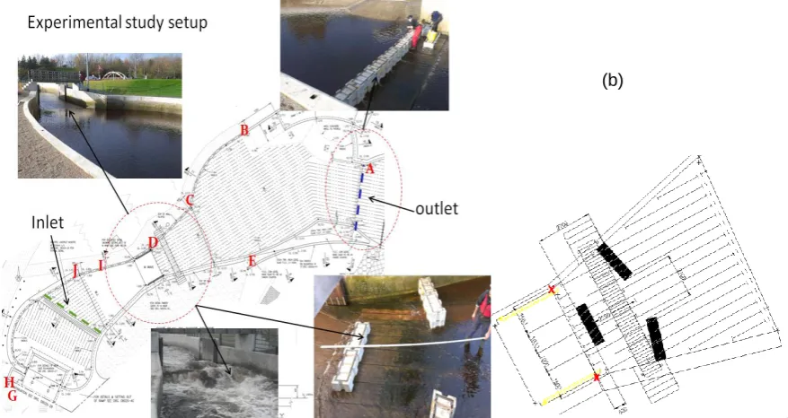
The test environment is a recreational white-water course that provides a means to vary the flow rates of water and restrict the flow as and when required. The physical channel is approximately 65m in length (from ‘inlet’ gate to downstream ‘outlet’ weir) with the channel bed having a fall of 3.1m over this length. The width of the channel ranges from approximately 4.5m to 23m. The flow rate of water into the channel is controlled by a movable gate that can be lowered incrementally to release water from the upstream channel. A StreamPro acoustic doppler current profiler (ADCP) is used to measure velocity profiles across the channel for each experimental trial, which in turn are used to calculate the flow rate for each experiment. A TLS (Topcon GLS 1500) was used to scan the empty channel bed and geometry and to record returns from the white-water.

Figure 2a provides an overview of the experimental channel with key features such as the location of the inlet gate and downstream weir identified. The weir height at the exit of the channel was initially set to 0.25m in height and in later studies was increased to 0.5m. Figure 2b shows a close-up view of the channel bed where the hydraulic jump is observed to form and where ‘obstacle blocks’ have been inserted onto the channel floor for the latter experiments.

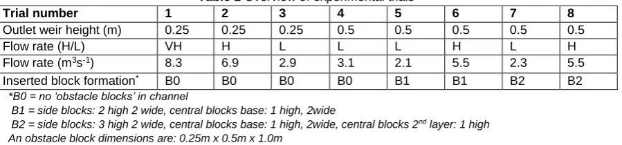
Table 1 outlines detail of seven experimental trials conducted. Trials 1-4 have no additional obstacle blocks inserted into the channel floor and involve varying the flow rate and downstream weir height. Trials 5 and 6 insert obstacle blocks into the channel as seen in the location set out in Figure 2b, for high and low discharge rates. Figure 4 and 5 are the same experiment, but with an increased height of block (on the same footprint). In each experiment a high (H) and low (L) flow was used; the absolute flow rate varied due to conditions over the 10 hour duration of the trial period. Low flows are between

2.1-3.1 m3_s-1 _{and high flow above 5.0 m}3_s-1_{. The block arrangement ‘B1’ can be observed in Figure 2.}

Table 1 Overview of experimental trials

Trial number 1 2 3 4 5 6 7 8

Outlet weir height (m) 0.25 0.25 0.25 0.5 0.5 0.5 0.5 0.5

Flow rate (H/L) VH H L L L H L H

Flow rate (m3_s-1_{) 8.3 6.9 2.9 3.1 2.1 5.5 2.3 5.5}

Inserted block formation* _{B0 B0 B0 B0 B1 B1 B2 B2}

*B0 = no ‘obstacle blocks’ in channel

B1 = side blocks: 2 high 2 wide, central blocks base: 1 high, 2wide

B2 = side blocks: 3 high 2 wide, central blocks base: 1 high, 2wide, central blocks 2nd _{layer: 1 high} An obstacle block dimensions are: 0.25m x 0.5m x 1.0m

2.2 Numerical Model

The solver Ansys Fluent 13.0 was selected for the numerical modelling as it provides robust and convenient implementation of the VOF-PLIC method. A RANS CFD approach is implemented in the work which incorporates an explicit VOF model to predict the transient free-surface behaviour of white-water. A description of the VOF-PLIC model is found in [17]. An initial pilot study is used to assess the approach including mesh requirements and sensitivity to turbulence model as required for the main study. In the main numerical study 3D numerical simulations are run for each of the experimental trials outlined in Table1. For the each case the boundary conditions used are based on the experiments with the water having a mass flow rate equated from the volume flow rate. Furthermore in each case the CFD is run transiently allowing the water to fill the channel and is left to run until a steady flow is reached.

Table 2 Overview of boundary conditions for main CFD study

Boundary Water phase Air phase

Inlet water Mass flow rate

(derived from flow rate in table 1)

n/a

Outlet Atmospheric pressure Atmospheric pressure

Walls No slip condition No slip condition

Atmosphere n/a Atmospheric pressure

3. RESULTS AND DISCUSSION

3.1 Pilot Study

The pilot modelling study carried out on a simplified geometry is used to evaluate the approach, assess the sensitivity of predictions to turbulence modelling and investigate mesh requirements. This study was performed on a simple 3D geometry in a 2m x 0.5m x 0.2m rectangular duct with a small 0.1m high block cut out of the channel bed. A dam break situation was simulated similar to that of Pracht (1997) with a block of water measuring 0.4m x 0.4m x 0.2m initially patched at one end of

the channel. The simulations were run transiently using the VOF-PLIC with the 𝑘 − 𝜖 RNG turbulence model and a

time-step of 0.005 seconds. Mesh independence was investigated with three mesh sizes of increasing size used- 25,000, 100,000, 225,000 elements. The finer of the 2 meshes are consistent for key aspects of the flow that is useful for understanding the mesh requirements for the full-scale study. Extrapolating from this study it was anticipated that for the full-scale study mesh elements of between 10-100mm in length would be required. In the main CFD study the base mesh used has 2.4 million elements with 55 elements in the vertical direction (z), 100 across the width (y) and 440 in the stream-wise direction (x).

Further simulations were undertaken to examine the effect of the turbulence model. In general, the simulations were

comparable with the 𝑘 − 𝜖 RNG and 𝑘 − 𝜔 SST models predicting the location of the free-surface generally more in line

with one another. Based on these tests and the previous literature the 𝑘 − 𝜖 RNG model will be used to model turbulence

3.2 Main Channel - Without Obstacles

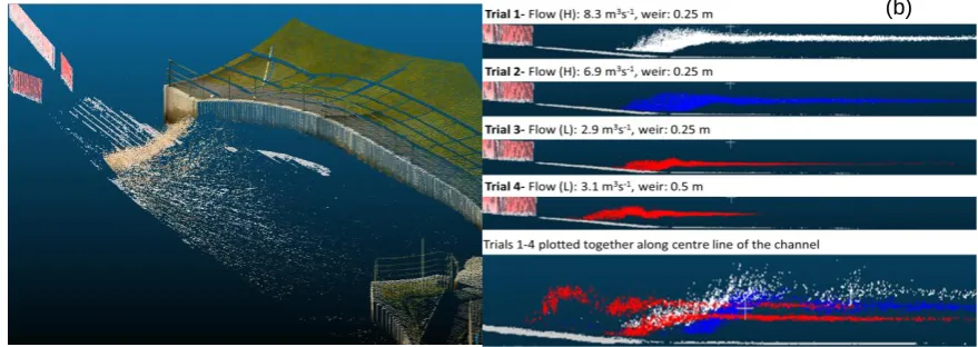
Before considering the examples with obstacles inserted in the channel, trials 1-4 were undertaken to investigate the location and shape of the stationary wave forming for different flow rates and downstream weir heights. The mesh used is a regular hexahedral structured mesh throughout. Figure 3a shows the point cloud data for experimental Trail 1. Both the channel and stationary wave are captured clearly using the TLS. Figure 3b shows the side profile of the point clouds for Trails 1-4. As expected the higher flow rates create a larger and more energetic hydraulic jump; however, the location at which the jump occurs is similar for each of the discharge rates. In the case of Trial 3 and 4, where the low discharge rate is used, the impact of increasing the downstream weir height is observed to move the location of the hydraulic jump upstream (as expected due to the higher water level it induces).

Figure 3 TLS point cloud of the channel (a) 3D view showing reflected white-water for trial 1, (b) horizontal plane view of white-water surface for Trials 1-4

Figure 4a and 4b show the process of overlaying the three-dimensional point cloud for the TLS measured white-water surface onto the the free-surface prediction for the VOF simulation. The case shown is for the low discharge rate and low downstream weir height (Trial 3). To aid analysis the point clouds can be separated into thin parallel strips. It can be observed that the model predicts the hydraulic jump well in terms of both position and height. This is further supported by the photograph shown in figure 4c which shows the forming hydraulic jump and provides a good visual comparison with the CFD and measured TLS data. A similar good level of agreement is also found for Trials 3 and 4.

Figure 4 Predictions for Trial 3 (a) TLS point cloud and CFD free-surface prediction shown together (b) The CFD prediction (c) a photograph of the hydraulic jump/stationary wave

3.3 Obstacle blocks inserted prior to the hydraulic jump

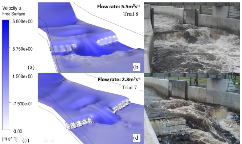
The two different obstacle block arrangements were simulated at both high and low discharge rates. Figure 5 shows the

(b)

Trial 3

(c) (b

example the water level over the blocks correctly simulated and the undular shape of the flow, and location of the rollers clearly identified. Furthermore, the location of the hydraulic jump after the obstructions is correctly predicted in terms of position, shape and height. A similar good result is observed for Trial 7, where for the lower discharge rate, there is both observed and simulated a reduction in flow over the side blocks compared with the high discharge case (figure 5c and 5d). Water levels are observed to be comparable and both the breaking wave that forms between the blocks and the shape and location of hydraulic jump are correct in the simulations. A similar level of good qualitative agreement for the free-surface location is also observed for Trials 5 and 6. Figure 6a shows the predicted free-surface location on a vertical plane down the centre of the channel for each of Trials 5-8. Figure 6b shows the same predictions in the region around the obstacles, at the same location, overlaid with the TLS measurements of the white-water surface. From this comparison it can be observed that although the main flow features are predicted well (for example the water levels, the slope of the water surface) the location of other features appears to be predicted too early along this central plane (for example the position of the wave undulation in Trail 6). However, it should be noted that these flows have a small degree of localised transient behaviour. This is observed both in the transient CFD runs and physical observations. As such, the CFD, TLS and photographic result are each a ‘snap-shot’ that are not exactly synchronised. This in part could be a cause of some small localised differences between the model and measurements. This will be investigated in more detail in the next steps of the work.

Figure 5 CFD free-surface predictions coloured by stream-wise velocity and associated photograph for Trial 8 (a), (b),

respectively and for Trial 7 (c), (d), respectively.

Figure 6 Free-surface location at the centre of channel for trials 5-8 (a) CFD free-surface predictions (b) CFD

predictions and experimental results in region around the obstacle blocks (red=CFD, blue=TLS). Trial 8

Trial 7 (a)

(c)

(b )

(d )

Trial 5

Trial 6

Trial 7

4. CONCLUSIONS

The results of the study demonstrate that, although computationally intensive, the free-surface CFD approach evaluated can reliably predict the key features of complex hydraulic behaviour in medium/large-scale open channel flow conditions. In order to reliably capture the full three-dimensional characteristics of the water free-surface a high resolution mesh (2.5 million+ cells) with time-steps in order of milliseconds is necessary (running for around 30-60 seconds of real-time simulation). There are numerous potential industrial application areas where this approach can be exploited. These include applications in the design of ‘play features’ at recreational white-water courses (such as Lee-Valley Olympic White-Water Centre) as well as providing a meaningful tool for design of river management systems.

REFERENCES

BUDWIG, R., MCLAUGHLIN, R. E., CLAYTON, S., SWEET, S. & GOODWIN, P. , Physical modeling of wave generation for the Boise River Recreation Park, Proceedings of the International Conference of Science and Information Technologies for Sustainable Management of Aquatic Ecosystems 2009: Conceptión, Chile.

LIN, F., SHEPHERD, D., SLACK, C., SHIPLEY, S. & NILSON, A. Use of CFD Modeling for Creating Recreational

Opportunities At the Calgary Bow River Weir. World Environmental and Water Resources Congress. 2008. Ahupua'a. PRACHT, W.E., CALCULATING THREE-DIMENSIONAL FLUID FLOWS AT ALL SPEEDS WITH AN

EULERIAN-LAGRANGIAN COMPUTING MESH. . Journal of Computational Physics, 17, 132-159, 1975. 17: p. 132-159

SHIPLEY, S., LAIRD, A., VANDERPOL, M., PHEIL, C. , The use of computer and physical modeling to evaluate and

redesign a whitewater park., in Whitewater Courses & Parks 20102010: Colorado, USA