Modelling household finances: A Bayesian approach to a multivariate two-part model

(1)

Modelling household

ﬁ

nances: A Bayesian approach to a

multivariate two-part model

Sarah Brown

a,

⁎

_{, Pulak Ghosh}

b

_{, Li Su}

c

_{, Karl Taylor}

a a

Department of Economics, University of Shefﬁeld, 9 Mappin Street, Shefﬁeld S1 4DT, UK

b_{Department of Quantitative Methods and Information Systems, Indian Institute of Management, Bangalore, India}

c_{MRC Biostatistics Unit, Cambridge Institute of Public Health, Cambridge Biomedical Campus, Robinson Way, Cambridge, CB2 0SR, UK}

a r t i c l e i n f o

a b s t r a c t

Article history:

Received 16 December 2014

Received in revised form 17 March 2015 Accepted 19 March 2015

Available online 26 March 2015

We contribute to the empirical literature on householdfinances by introducing a Bayesian multivar-iate two-part model, which has been developed to further our understanding of householdfinances. Ourflexible approach allows for the potential interdependence between the holding of assets and liabilities at the household level and also encompasses a two-part process to allow for differences in the influences on asset or liability holding and on the respective amounts held. Furthermore, the framework is dynamic in order to allow for persistence in householdfinances over time. Our findings endorse the joint modelling approach and provide evidence supporting the importance of dynamics. In addition, wefind that certain independent variables exert different influences on the binary and continuous parts of the model thereby highlighting theflexibility of our framework and revealing a detailed picture of the nature of householdfinances.

JEL classiﬁcation: C11

G11 G21 Keywords: Assets

Bayesian approach Bridge distribution Debt

Two-part model

1. Introduction

Over the last three decades, there has been growing interest in thefinancial economics literature in the nature offinancial portfolios at the household level. Such interest has coincided with significant changes in debt and asset accumulation at the household level. Over the last decade, for example, there has initially been a considerable increase in consumer debt in the U.S. followed by a decline in household leverage, the ratio of debt to disposable income, with the onset of the recession towards the end of 2007,Glick and Lansing (2009)and

Brown et al. (2013). In general, in the existing literature, economists have focused on speci_fic aspects of the_financial portfolio including the demand for riskyfinancial assets such as stocks and shares (for example,Bertaut, 1998, Hochguertel et al., 1997andShum and Faig, 2006), savings (for example,Browning and Lusardi, 1996) or debt (for example,Brown et al., 2005, 2008, andCrook, 2001).

Policy-makers have, however, commented on the importance of analysing household_financial assets and liabilities together, which is at odds with the approach generally taken in the academic literature which explores specific aspects of household finances in isolation of other aspects of the household balance sheet. In particular, Alan Greenspan, the former chairman of the U.S. Federal Reserve Board, has argued that unless one simultaneously considersfinancial assets along with liabilities it is hard to ascertain the true burden of debt.1_{Similarly, the Monetary Policy Committee in Great Britain has acknowledged the}

⁎Corresponding author.

1_{Remarks made by Alan Greenspan}_“_{Understanding Household Debt Obligations}_”_{at the Credit Union National Association, Government Affairs Conference, Washington,} D.C. February 23, 2004.

http://dx.doi.org/10.1016/j.jempﬁn.2015.03.017

Contents lists available atScienceDirect

Journal of Empirical Finance

(2)

importance of establishing whether the same households have been accumulatingﬁnancial assets as well as debt over the recent years (Bank of England, Minutes of the Monetary Policy Committee, 2002andBrown and Taylor, 2008).

One exception in the academic literature isCox et al. (2002), who explorefinancial pressure across households in Great Britain, and find that households with the highest absolute levels of debt also tend to have the highest income and net wealth, implying that these households may be relatively well disposed towards coping with adverse_financial shocks. On the other hand, the_findings ofBrown and Taylor (2008), who jointly model household debt and assets, suggest that the youngest households and those households who are in the lowest income quartile are the most vulnerable to changes in theirfinancial circumstances since a high proportion of them hold debt yet nofinancial assets, i.e. they have negative net worth. Suchfindings highlight the importance of further research in this area. Moreover, it is apparent that, in order to predict the influences of changes in economic policy at the household level, such as changes in the interest rate, it is important to adopt a holistic approach to analysing householdfinances including both assets and liabilities.

In order to contribute to the literature on householdfinances, we analyse panel data from the U.S. Panel Study of Income Dynamics (PSID), for 1984, 1989, 1994, 1999, 2001, 2003, 2005, 2007, 2009 and 2011, with our period of analysis covering pre and post the recentfinancial crisis. The PSID provides detailed information at the household level as well as allowing us to track households over time. In addition to providing empirical analysis of householdfinances during this period, we develop aflexible empirical frame-work, which reveals a detailed picture of liability and asset holding at the household level and allows us to uncover interdependencies across the various aspects of householdfinances. We adopt a Bayesian approach, which is highlyflexible in the context of complex models. Hence, given the complicated nature of householdfinances, it is surprising that there is a lack of Bayesian analysis in the existing literature. Many of the statistical models used in the existing literature treat the level of household debt or assets as censored variables since they cannot have negative values. Consequently, a Tobit approach has been commonly used to allow for this truncation (see, for example,Bertaut and Starr-McCluer (2002)andBrown et al. (2005, 2008)). In studies, where a joint modelling approach has been adopted, a bivariate Tobit model has been used allowing for the possibility of inter-dependent decision-making with respect to financial assets and liabilities (see, for example,Brown and Taylor (2008), where thefindings endorse the joint modelling approach indicating interdependence between the holding of assets and debt).2_{One problem with the Tobit approach, however, lies in the} possibility that the decision to hold debt orfinancial assets and the decision regarding the level of debt orfinancial assets held may be characterised by different influences. In terms of evaluating the level offinancial pressure faced by households, there is a significant difference, for example, between being in debt and holding high amounts of debt.

A double-hurdle model is an alternative econometric specification, which allows independent variables to have different effects on the probability of holding debt orfinancial assets and on the level of debt orfinancial assets if it is non-zero. Such an approach allows for a two-stage decision-making process: for example, a household decides whether to hold a particular asset and, conditional on the decision to hold a particular asset, the household then decides how much of that asset to hold, where there is potential correlation between the two decision-making processes (see, for example,Yen et al. (1997), in the context of analysingfinancial donations). The double-hurdle model has not, however, been extended to the multivariate case. Thus, studies adopting the double-hurdle approach have been restricted to focusing on one aspect of householdfinances. It is clearly important to allow for different aspects of householdfinances: for example, as stated above, it may not be problematic in terms of levels offinancial vulnerability if households holding debt simultaneously hold assets to draw upon if an adverse event arises.

In this paper, we develop aflexible Bayesian multivariate two-part model for the joint modelling of four aspects of household finances, namely unsecured debt, secured debt, non-housingfinancial assets and housing assets. With correlated random effects, our approach allows for the potential interdependence between household liabilities and asset holding and, hence, allows for poten-tial complex interactions between the various components of householdfinances, as well as persistence over time. This is important given that policy-makers have highlighted such interdependence as being relevant for ascertaining the truefinancial health of or burden faced by households, i.e. it is important to consider debt levels in the context of asset holdings and vice versa. In addition, our approach incorporates a two-part process which allows for differences in the effects of the explanatory variables on the decision to acquire assets or debt and on the amount of assets or debt held.

The results from our new framework endorse the joint modelling approach and provide evidence supporting dynamics in asset and debt holding at the household level. In addition, our results indicate that certain independent variables exert different influences on the binary and continuous parts of the model. The results are potentially interesting from a policy perspective. For example, wefind evidence of strong persistence in the probability of households holding unsecured debt: if the head of household held unsecured debt in the previous period the likelihood of currently holding such debt increases by 126 percentage points. Hence, if alleviating the number of individuals in debt is a concern, policymakers may consider influencing the underlying behaviour of households or the mechanisms behind how credit is obtained, such as from a high street bank or a pay-day loan company, where the latter is likely to be more accessible but carries higher risk in terms of the rate of interest required, which may exacerbate future debt levels.

2. Empirical framework

In this section, we develop a Bayesian multivariate two-part model for the joint modelling of four aspects of household ﬁnances, namely unsecured debt, secured debt, non-housingﬁnancial assets and housing assets. By two-part model, we refer to data generated from a response which is a mixture of true zeros and continuously distributed positive values (Olsen and

(3)

Schafer, 2001; Tooze et al., 2002). We adopt a Bayesian estimation strategy, which has the following distinct advantages for our model. First, our Bayesian estimation procedure, with the incorporation of the recent development of the Markov Chain Monte Carlo (MCMC) method (Gelfand and Smith, 1990), is powerful andﬂexible in dealing with complex non-linear problems, where the classical maximum likelihood approach encounters severe computational difﬁculties (Lopes and Carvalho, 2013). Second, the Bayesian strategy enables us to examine the entire posterior distribution of the parameters, and avoid the dependence on asymptotic properties to assess the sampling variability of the parameter estimates.

With correlated random effects, the proposed approach allows for the potential interdependence between the holding of assets and debt at the household level, and also encompasses a two-part process to allow for differences in the influences of the independent variables on the decision to hold debt or assets and the influences of the independent variables on the amount of debt orfinancial as-sets held. The model also incorporates dynamics in the two-part process, i.e. the decision to acquire and the amount held, hence allowing for persistence over time. In addition to the novelty of introducing a Bayesian approach to exploring the influences on house-holdfinances, combining the joint modelling approach with the two-part approach brings together two important aspects of house-holdfinancial decision-making which have been explored separately in the literature to date.

In terms of the specific statistical methods proposed in this paper, our multivariate two-part model has the advantage of offering straightforward interpretations of the effects of the independent variables, both conditionally (i.e., given the random effects) and mar-ginally (i.e., after integrating over the random effects), when modelling the binary parts of household balance sheet. In the standard generalized linear mixed model (GLMM) for binary dependent variables, the marginal probabilities integrated over Normal random effects in general no longer follow a generalized linear model (GLM) if a non-linear link function (e.g., logit link) is adopted (Diggle et al. 2002). In this case, the GLMM with Normal random effects can only provide subject-specific effects of independent variables con-ditional on random effects, whilst the population-averaged effects of independent variables on marginal probabilities might be of in-terest for the study in question. Therefore, in practice it is desirable that both the population-averaged and subject-specific effects of independent variables are readily available when drawing study conclusions. For this purpose, instead of using the usual Normal dis-tribution, we use the bridge distribution introduced inWang and Louis (2003)for the random intercepts in the binary parts of the dependent variables. The bridge distribution allows both the marginal model (integrated over the distribution of the random inter-cept) and the conditional model (conditional on the random effects) for the binary parts of the dependent variables to follow a logistic regression model, with regression coefficients proportional to each other.

Specifically, in our two-part model for a single dependent variable (e.g., unsecured debt), we use a random intercept logistic model for modelling the binary part of the dependent variable and a random intercept Gamma GLMM with a log link for modelling the con-tinuous part of the dependent variable. As mentioned earlier, the random intercept in the conditional logistic model for the binary part follows a bridge distribution, whilst the random intercept in the Gamma GLM for the continuous part follows a Normal distribution (Lin et al. 2010; Su et al. 2015; Wang and Louis, 2003). The marginal effects of the independent variables are proportional to the con-ditional effects of the independent variables with closed forms in both parts of the model because the marginal expectations in both parts preserve the logit and log links after integration over the random effects. The same two-part model is specified for the other de-pendent variables, i.e. secured debt; non-housingfinancial assets and housing assets. The interdependence between the two parts of each dependent variable as well as the interdependence between all of the dependent variables is taken into account by allowing the random effects to be correlated. Further, a multivariate density using a Gaussian copula model is assumed for the random effects, which is parameterised by the correlation matrix of the Gaussian copula and marginal variances of the random effects. Due to the mul-tivariate nature of our data, the correlation matrix of the Gaussian copula is left as unstructured, where the new partial autocorrelation approach is adopted to guarantee the positive definiteness of the correlation matrix (Daniels and Pourahmadi, 2009).

2.1. Modelling the value of unsecured debt

Letyijudbe the unsecured debt of theith household (i= 1,2,…,n) in thejth wave (j= 1,2,…,m) wherenis the total number of house-holds andmis the total number of follow-up waves. LetRijudbe a random variable denoting whether unsecured debt is held where

Rudi j ¼

0 ifyudi j ¼0 1 ifyudi jN0

(

with

prob Rudi j ¼r ud i j

¼ 1−p ud i j if r

ud i j ¼0 pudi j if r

ud i j ¼1:

(

Further, letsijud≡[yijud|Rijud= 1] denote the positive unsecured debt of theith household in thejth wave.

We model the probabilitypijud(the‘binary part’of the model) using a random intercept logistic model and the non-zero continuous observationssijud(the‘continuous part’of the model) using a Normal GLMM with a log link as follows:

logit pudi j

¼X1

i jβ

1

þη1y

ud i;j−1þB

ud i

log sudi j N μ ud i j;σ

ud2

i

μud i j ¼X

2

i jβ

2

þη2y

ud i;j−1þV

ud i

(4)

whereXij1andXij2are the independent variable vectors with associated parametersβ1andβ2for the binary and continuous parts, re-spectively; andBiudandViudare the random intercepts of the two parts of the model accounting for the dependence of the repeated observations within the household.

2.2. Modelling the value of secured debt

Letyijsdbe the secured debt of theith household (i= 1,2,…,n) in thejth wave (j= 1,2,…,m). LetRijsdbe a random variable denoting whether secured debt is held where

Rsdi j ¼

0 if ysdi j ¼0 1 if ysdi jN0

(

with

prob Rsdi j ¼r sd i j

¼ 1−p sd i j if r

sd i j ¼0 psdi jif r

sd i j ¼1:

(

Further, letsijsd≡[yijsd|Rijsd= 1] denote the positive secured debt of theith household in thejth wave.

We model the probabilitypijsd(the‘binary part’of the model) using a random intercept logistic model and the non-zero continuous observationssijsd(the‘continuous part’of the model) using a Normal GLMM with a log link as follows:

logit psdi j ¼X

3

i jβ

3

þη3y

sd i;j−1þB

sd i

log ssdi j N μ sd i j;σ

sd2

i

μsd i j ¼X

4

i jβ

4_þ

η4y

sd i;j−1þV

sd i

ð2Þ

whereXij3andXij4are the independent variable vectors with associated parametersβ3andβ4for the binary and continuous parts, respectively; andBisdandVisdare the random intercepts of the two parts of the model accounting for the dependence of the repeated observations within the household.

2.3. Modelling the value of non-housingﬁnancial assets

Letyijfabe theﬁnancial assets, excluding the value of housing, of theith household (i= 1,2,…,n) in thejth wave (j= 1,2,…,m). Let Rijfabe a random variable denoting whetherﬁnancial assets are held where

R_{i j}f a¼ 0;ify f a i j ¼0 1 if yi jf aN0

(

with

probR_{i j}f a¼r_{i j}f a¼ 1−p f a i j ifr

f a i j ¼0 pi jf aifr

f a i j ¼1:

(

Further, letsij fa

≡[yijfa|Rijfa= 1] denote the positiveﬁnancial assets of theith household in thejth wave.

We model the probabilitypijfa(the‘binary part’of the model) using a random intercept logistic model and the non-zero continuous observationssijfa(the‘continuous part’of the model) using a Normal GLMM with a log link as follows:

logit pi jf a

¼X5

i jβ

5

þη5y

f a i;j−1þB

f a i

log si jf a N μ f a i j;σ

f a2

i

μf a i j ¼X

6

i jβ

6

þη6y

f a i;j−1þV

f a i

ð3Þ

(5)

2.4. Modelling the value of housing assets

Letyijhabe the house value of theith household (i= 1,2,…,n) in thejth wave (j= 1,2,…,m). LetRijhabe a random variable denoting whether housing assets are held where

Rhai j ¼

0 if yhai j ¼0 1 if yhai jN0

(

with

prob Rhai j ¼r ha i j

¼ 1−p ha i j if r

ha i j ¼0 phai j if r

ha i j ¼1:

(

Further, letsijha≡[yijha|Rijha= 1] denote the value of housing assets, conditional on such assets being held, of theith household in the jth wave.

We model the probabilitypijha(the‘binary part’of the model) using a random intercept logistic model and the non-zero continuous observationssijha(the‘continuous part’of the model) using a Normal GLMM with a log link as follows:

logit phai j

¼X7

i jβ

7

þη7y

ha i;j−1þB

ha i

log shai j N μ ha i j;σ

ha2

i

μha i j ¼X

8

i jβ

8_þ

η8y

ha i;j−1þV

ha i

ð4Þ

whereXij7andXij8are the independent variable vectors with associated parametersβ7andβ8for the binary and continuous parts, respectively; andBihaandVihaare the random intercepts of the two parts of the model accounting for the dependence of the repeated observations within the household.

Note that for each of the continuous outcomes we incorporate heteroscedasticity in the error terms, i.e. (σiud)2, (σsdi )2, (σifa)2and (σiha)2in Eqs.(1) to (4), respectively. By assuming a prior on the variance, this enables the variance to be random across households and hence household speciﬁc.

2.5. Random effects model

For each household, we have an 8-dimensional random effect vectorbi= (Biud,Vudi ,Bisd,Visd,Bifa,Vifa,Biha,Viha)T. Since the binary and continuous parts of the sub-models are highly likely to be related within the households over the follow-up waves, it is necessary to allow the elements ofbito be correlated. A typical option would be to assume a multivariate normal distribution forbi. However, the logistic models in Eqs.(1) to (4)with normal random effects can only provide the household speciﬁc independent variable effects conditional on the random effects. In order to provide marginal effects of the independent variables in the logistic models for the binary outcomes, we extend the random intercept GLMM approach inWang and Louis (2003)to the multivariate two-part model setting.

We assume thatBiud,Bisd,BifaandBiha, the random intercepts in the binary parts, marginally follow the bridge distributions ofWang and Louis (2003)with densities

f1 b

ud i jϕ1

¼ 1 2π

sinðϕ1πÞ cosh _ϕ1budi

þcosð_ϕ1πÞ

−∞bbudi b∞

f3 b

sd i jϕ3

¼ 1 2π

sinð_ϕ3πÞ

cosh ϕ3bsdi

þcosðϕ3πÞ

−∞bbsdi b∞

f5 b

f a i jϕ5

¼ 1 2π

sinðϕ5πÞ cosh ϕ5b

f a i

þcosðϕ5πÞ

−∞bbif ab∞

f7 b

ha i jϕ7

¼ 1 2π

sinðϕ7πÞ

cosh ϕ7bhai

þcosðϕ7πÞ

−∞bbhai b∞

(6)

variables through the same logit link functions as for the corresponding conditional probabilities. In addition, if we specify the marginal regression structure of the binary parts as

logit prob Rudi j ¼1

n o

¼Xi jθ

1

logit prob Rsdi j ¼1

n o

¼Xi jθ

3

logit probn R_{i j}f a¼1o¼Xi jθ

5

logit prob Rhai j ¼1

n o

¼Xi jθ

7

then the marginal independent variable effectsθk_(k_{= 1, 3, 5, 7) are proportional to the household speci}_ﬁ_{c conditional} inde-pendent variable effectsβk_with_θk₌_ϕ

kβk. Therefore models(1) to (4)can be rewritten as

logit prob Rudi j ¼1B ud i n o

¼X1

i jθ

1

=ϕ1þB

ud

i ð5Þ

logit prob Rsdi j ¼1B sd i n o

¼X3

i jθ

3

=ϕ3þB

sd

i ð6Þ

logit prob Ri jf a¼1B f a i n o

¼X5

i jθ

5

=ϕ5þB

f a

i ð7Þ

logit prob Rhai j ¼1B ha i n o

¼X7

i jθ

7

=ϕ7þB

ha

i : ð8Þ

Further,Viud,Visd,VifaandVihaare assumed to be marginally normally distributed with mean zero and variance,τud2,τsd2,τfa2andτha2, re-spectively. Therefore, log(sijud), log(sijsd), log(sijfa) and log(sijha), given the vector of random effectsbi= (Biud,Viud,Bisd,Visd,Bifa,Vfai,Biha,Viha)T, follow GLMM with means (Xij2β2+Viud), (Xij4β4+Visd), (Xij6β6+Vifa) and (Xij8β8+Viha), respectively.

For the purpose of characterizing the interdependence of the dependent variables and the possible dependence between the two parts, as well as assuring the desired marginal density of each member ofbi, we construct a multivariate joint distribution for the ran-dom effects using a Gaussian copula, seeNelsen (1999). A copula is a convenient way of formulating a multivariate distribution, and is speciﬁed as a function of the marginal cumulative distribution function (CDF). IfF1(biud),F2(υiud),F3(bisd),F4(υisd),F5(bifa),F6(υifa), F7(biha) andF8(υiha) are the CDFs ofbi= (Biud,Viud,Bsdi ,Visd,Bifa,Vifa,Biha,Viha)T, respectively, then there exists a functionCsuch that the joint CDF ofbiisF(biud,viud,bisd,visd,bifa,vifa,biha,viha) =C{F1(biud),F2(viud),F3(bsdi),F4(visd),F5(bifa),F6(vifa),F7(biha),F8(viha)}, see Nelsen (1999)andJoe (1997).

To construct the Gaussian copula forbi, we specify a vectorUi= (Ui1,Ui2,Ui3,Ui4,Ui5,Ui6,Ui7,Ui8)Tsuch that

Ui1 Ui2 Ui3

⋮

Ui8 2 6 6 6 6 4 3 7 7 7 7 5N

0 0 0 ⋮ 0 2 6 6 6 6 4 3 7 7 7 7 5; Σ¼

1 ρ12 ρ13 ⋯ ρ18

ρ21 1 ρ23 ⋯ ρ28

ρ31 ρ32 1 ⋯ ρ38

⋮ ⋮ ⋮ ⋱ ⋮

ρ81 ρ82 ρ83 ⋯ 1 2 6 6 6 6 4 3 7 7 7 7 5 0 B B B B @ 1 C C C C

A: ð9Þ

Note that the diagonal elements of the covariance matrixΣare equal to 1 so that it is also the correlation matrix. We letρj,j+t= corr(Uij,Ui,j+t), wherej= 1, 2,.., 8; 1≤t≤8, denote the correlation betweenUijandUi,j+t. Using the probability integral transforms (seeHoel et al. (1971)), thenBiud=F1−1{Φ(Ui1)},Bisd=F3−1{Φ(Ui3)},Bifa=F5−1{Φ(Ui5)} andBiha=F7−1{Φ(Ui7)} have marginal CDFs of F1(biud),F3(bisd),F5(bfai) andF7(biha), respectively (seeLin et al. (2010), andWang and Louis (2003)). HereΦ(⋅) is the standard normal CDF, andFk−1(⋅) (k= 1, 3, 5, 7) is the inverse cumulative distribution function,

F−k1ð Þ ¼x 1

ϕk

log sinðϕkπxÞ sinfϕkπð1−xÞg

(7)

3. Bayesian inference

3.1. Likelihood speciﬁcation

Let_Yiud= (yi1ud,…,yimud)T,Yisd= (yi1sd,…,yimsd)T,Yifa= (yi1fa,…,yimfa)TandYiha= (yi1ha,…,yimha)T. Similarly, we deﬁneXik= (Xki1,…,Ximk)T fork= 1,2,...,8. LetΩ1= (β1,β2),Ω2= (β3,β4),Ω3= (β5,β6),Ω4= (β7,β8) be the vectors for the multivariate dependent variables, Ω5= (ϕ1,τud,ϕ3,τsd,ϕ5,τfa,ϕ7,τha) be the parameter vector for random effectsbi= (Biud,Viud,Bisd,Visd,Bifa,Vifa,Biha,Viha)T. The likelihood function for theith household can be partitioned as

L Ω1;Ω2;Ω3;Ω4;Ω5Y

ud i ;Y

sd i ;Y

f a i ;Y

ha i ;X

1

i;X

2

i;X

3

i;X

4

i;X

5

i;X

6

i;X

7

i;X

8 i bi ∝

L Ω1Y

ud i ;X

1

i

;X2

i;B ud i ;V

ud i

L Ω2Y

sd i ;X

3

i

;X4

i;B sd i ;V

sd i

L Ω3Y

f a i ;X

5

i

;X6

i;B f a i ;V

f a i

L Ω4Y

ha i ;X

7

i

;X8

i;B ha i ;V

ha i

L Ω5B

ud i ;V

ud i ;B

sd i ;V

sd i ;B

f a i ;V

f a i ;B

ha i ;V

ha i

ð10Þ

where

L Ω1Y

ud i ;X

1

i

;X2

i;B ud i ;V

ud i

¼ ∏m

j¼1

1−prob Rudi j ¼1B ud i

n o1−rud

i j

ð Þ

prob Rudi j ¼1B ud i

LN Yudi j;μ ud i j;σ

ud2 i

rudi j

L Ω2Y

sd i ;X

3

i

;X4

i;B sd i ;V

sd i

¼ ∏m

j¼1

1−prob Rsdi j ¼1B sd i

n o1−rsd

i j

ð Þ

prob Rsdi j ¼1B sd i

LN Ysdi j;μ sd i j;σ

sd2 i

rsdi j

L Ω3Y

f a i ;X

5

i

;X6

i;B f a i ;V

f a i

¼ ∏m

j¼1

1−probR_{i j}f a¼1B_if a

n o 1−rf a

i j

probR_{i j}f a¼1B_if aLN Y_{i j}f a;μf a i j;σ

f a2

i

rf a

i j

L Ω4Y

ha i ;X

7

i

;X8

i;B ha i ;V

ha i

¼ ∏m

j¼1

1−prob Rhai j ¼1B ha i

n o1−rha

i j

ð Þ

prob Rhai j ¼1B ha i

LN Yhai j;μ ha i j;σ

ha2

i

rha

i j

withμijud,μijsd,μijfaandμijhagiven in Eqs.(1) to (4)respectively, and

L Ω5B

ud i ;V

ud i ;B

sd i ;V

sd i ;B

f a i ;V

f a i ;B

ha i ;V

ha i

¼C F1 b

ud i

; F2 υ

ud i

; F3 b

sd i ; F4 υ

sd i

; F5 b

f a i

; F6 υ

f a i

; F7 b

ha i

; F8 υ

ha i

n o

f1 b

ud i jϕ1

ϕ υ ud i τud !

f3 b

sd i jϕ3

ϕ υ sd i τsd !

f5 b

f a i jϕ5

ϕ υ f a i τf a

!

f7 b

ha i jϕ7

ϕ υ ha i τha !

ð11Þ

withfk(⋅)k= 1, 3, 5, 7 being the bridge density functions,ϕ(⋅) being the standard normal density function andc(⋅) being the density of the copulaC(⋅) fromSection 2.5. This is given by

cðqjΣÞ ¼j jΣ−1=2 exp 1

2u T

I−Σ−1

u

:

Hereq= (q1,…,q8) with (0bqkb1, k= 1,…, 8),u= (u1,…, u8)Ta vector of normal scoresuk=Φ−1(qk), andIis an 8-dimen-sional identity matrix.

3.2. Prior speciﬁcation and posterior inference

To complete the Bayesian speciﬁcation of the model, priors need to be assigned for all unknown parameters. We assume that the elements ofΩ1,Ω2,Ω3,Ω4, andΩ5, are independently distributed. Because the number of independent variables is large in the joint model, they might be expected to have weak effects on the dependent variables. In order to incorporate this prior knowledge into our analysis, we set up a prior distribution such that each regression coefﬁcient has a high probability of being near zero but a large effect is still possible.

A commonly used prior in this scenario is the Laplace prior or double exponential prior to obtain shrinkage estimates. The Laplace prior for ap× 1 regression coefﬁcient vectorβis given by the following:

fðβ;ψÞ ¼ ∏p

j¼1

ψ

2exp −ψ βj

(8)

The above LASSO shrinks all the parameters to the same degree. However, when some effects are non-null, shrinkage towards these non-null locations may be beneﬁcial.3_{Thus, we extend the above LASSO speci}_ﬁ_{cation using a newly developed Bayesian} adaptive shrinkage LASSO prior proposed byMacLehose and Dunson (2010). We assume the following prior

βjψjN μj;ψj

ψj exp 2=λj

μj;λj

θδ μjj0

Gamma λjja0;b0

þð1−θÞN μjjc;d

Gamma λjja1;b1

θBeta 1ð ;1Þ

ð12Þ

where_δ(_μj|0) indicates thatμjhas a degenerate distribution with all its mass at 0. With probabilityθ, the coefﬁcientβjis shrunk towards zero as in the standard LASSO model. With probability (1−θ), the coefﬁcientβjis shrunk towards non-zero mean,μj. The amount of shrinkage is determined byλjwith large values resulting in greater shrinkage. We specifya0andb0to give support to large values ofλjin order to allow for strong shrinkage ofβjtowards 0, whilst specifyinga1andb1to give support to smaller values ofλjto allow less shrinkage towards non-zero values.

In the analysis shown inSections 2.1to 2.4, all elements of the regression coefﬁcient vectors,β1_,_β2_,_β3_,_β4_,_β5_,_β6_,_β7_and_β8_are assigned an adaptive LASSO prior. FollowingMacLehose and Dunson (2010), we assume,a0=b0= 30 anda1=b1= 7. For param-eters in the random effects model, denoteτ12=π2(ϕ1−2−1)/3,τ32=π2(ϕ3−2−1)/3,τ52=π2(ϕ5−2−1)/3 andτ72=π2(ϕ7−2−1)/3 and we use the following priorsτ1,τud,τ3,τsd,τ5,τfa,τ7andτha, iid ~ uniform(0,10). Finally, independent uniform priors on [−1,1] (or beta(2,1) priors transformed to [−1,1]) are chosen for the partial autocorrelationsγ12,γ13,γ14,γ15,γ16,γ17,γ18,γ23,γ24,γ25,γ26,γ27, γ28,γ34,γ35,γ36,γ37,γ38,γ45,γ46,γ47,γ48,γ56,γ57,γ58,γ67,γ68andγ78. We assume a weakly informative Gamma prior distribution for error variances, (σiud)2., (σisd)2, (σifa)2and (σiha)2.

The joint posterior distribution of the model parameters conditional on the observed data are obtained by combining the likelihood fromSection 3.1and the previously speciﬁed priors using Bayes Theorem:

POST Ω1;Ω2;Ω3;Ω4;Ω5;biY ud i ;Y

sd i ;Y

f a i

Yha

i

∝ ∏n

i¼1

Li Ω1;Ω2;Ω3;Ω4;Ω5Y

ud i ;Y

sd i ;Y

f a i

Yha

i ;bi

fð Þbi fðβ ψj ;θÞfð Þθfð Þτ1 fðτudÞ

fð Þτ3 fðτsdÞfð Þτ5 f τf a

fð Þτ7 fðτhaÞfð Þγ f σ ud2 i

f σsd2 i

f σf a2 i

f σha2 i

:

ð13Þ

The posterior distributions are analytically intractable. However, computation can be achieved using MCMC methods such as the Gibbs sampler (Gelfand et al., 1992). Since all the full conditional distributions are not standard, a straightforward implementation of the Gibbs sampler using standard sampling techniques may not be possible. However, sampling methods can be performed using Adaptive Rejection Sampling (ARS), metropolis hastings and/or blocked Gibbs sampling methods (Gilks and Wild, 1992).

In this paper we have used a general program for Bayesian inference using Gibbs Sampling implemented in the WinBUGS package (version 1.4.1),Spiegelhalter et al. (1996). WinBUGS uses the Gibbs sampling algorithm to construct transition kernels for its Markov chain samplers. During compilation, WinBUGS chooses a method to draw samples for each of the full conditional distributions of the model parameters. Such sampling can be done univariately or in multivariate nodes. The sampling methods within WinBUGS include di-rect sampling using standard algorithms, derivative free ARS (Gilks, 1992), slice sampling (Neal, 2000) and metropolis sampling (Gelfand and Smith, 1990) and blocked Gibbs sampling. The_first choice is always a standard density if it is available. This possibility arises when a full conditional is recognizable. For non-standard but log-concave full conditionals, ARS sampling is used to sample the full conditional (Gilks and Wild, 1992). WinBUGS checks if log-concavity is satisfied or not, and uses slice sampling if this condition is not met (Neal, 2000). The random walk metropolis algorithm is also used by WinBUGS for non-conjugate continuous full conditionals. The samples from the posterior distribution obtained from the MCMC allow us to achieve summary measures of the parameter estimates. Summary statistics such as posterior means and statistical significance obtained from 95% credible intervals are provided for inference.

3.3. Model selection

For comparing between alternative models, we use a selection criteria called Deviance Information Criteria (DIC) proposed bySpiegelhalter et al. (2002). This approach has been used in several previous studies involving zero-inﬂated data (such as

Neelon et al. (2010);Montagna et al. (2012)). As with the Akaike Information Criterion (AIC) and the Bayesian Information Criterion (BIC), the DIC also provides an assessment of modelfit and a penalty for model complexity. Letθbe the set of parameters in a model, then the DIC is de_fined asDð Þ þ_θ pD, whereDð Þ ¼θ E D½ ð Þθjyis the posterior mean of the deviance, D(θ), and pD¼Dð Þθ−D^ð Þ ¼θ E D½ ð Þθjy−D Eð ½θjyÞis the difference in the posterior mean of the deviance and the deviance evaluated at the posterior mean of the set of parameters. The deviance is taken as negative twice the log-likelihood and is a measure of a model's relativefit, whereaspDis a penalty for the model's complexity (Montagna et al., 2012). Whilst the AIC and the BIC are well suited forfixed effects models (since the number of parameters are easily determined), for the hierarchical random effects model the DIC is better suited as the dimension of the parameter space is less clear and depends on the degree of

3

(9)

heterogeneity between subjects (Montagna et al., 2012). The DIC was proposed to estimate the number of effective parameters in a Bayesian hierarchical model. Forﬁnite mixture models,Celeux et al. (2006)proposed a modiﬁed DIC, termed DIC3, since in a mixture distribution the effective number of parameters,pD, can be negative. The DIC3estimatesD^ð Þθ using the posterior mean of the marginal likelihood and is given by DIC3¼2Dð Þ þθ 2 log∏ni^f yð Þi

h

, where^fð Þyi is the posterior mean of the marginal likeli-hood contribution for subjecti. A smaller DIC denotes a better model. If two models differ by more than ten, then the one with the smaller DIC is considered the bestﬁt (Spiegelhalter et al., 2002).

We also use an alternative model selection criteria–the cross validated predictive approach ofGelfand et al. (1992), i.e. the predictive distributions conditioned on the observed data with a single data point deleted. The conditional predictive coordinate (CPO) has been widely used for model diagnostic and assessment (Chen et al., 2000; Gelfand et al., 1992) and for our model is deﬁned as:

CPOi¼p Y P i;Y

C i;ViY

P

−i;YC−i;V−i

¼E_θ p YP i;Y

C i;Vijθ

YP −i;Y

C −i;V−i

h i

wherep(YiP,YiC,Vi|Y−iP ,Y−iC,V−i) is the posterior predictive density ofp(YiP,YiC,Vi) for subjecticonditional on the observed data with a single data point deleted,_θdenotes all unobservables in the model under consideration, and the expectation is taken with respect to the posterior distribution ofθconditional onp(Y−iP ,Y−iC,V−i).Gelfand et al. (1992)have proposed a harmonic mean estimator ofCPOi based on Markov chain samples from the full posterior given the entire data,y.Geisser and Eddy (1979)andGelfand et al. (1992)

proposed the pseudo-marginal likelihood∏p(YiP,YiC,Vi|Y−iP ,Y−iC,V−i) or its logarithm, i.e. the Log Pseudo Marginal Likelihood (LPML):

LPML¼Xn i¼1logp Y

P i;Y

C i;ViY

P

−i;YC−i;V−i

:

Higher values of the LPML denote a superior speciﬁcation. In our analysis we use the DIC and LPML to select between competing models.

4. Modelling householdﬁnances

4.1. Data

Using the proposed model, we analyse data collected from the U.S. Panel Study of Income Dynamics (PSID). The PSID is an ongoing panel study of households conducted at the Institute for Social Research, University of Michigan since 1968. The sample size has grown from 4800 families in 1968 to more than 7000 families by the turn of the century. Further information on the PSID is available at:

http://psidonline.isr.umich.edu. Our data set contains information on: unsecured debt, e.g. credit card debt, (yijud); secured debt, e.g. mortgage debt, (yijsd); non-housingfinancial assets, e.g. stocks and shares, (yijfa); and housing assets (yijha). We analyse this information for a balanced panel of households measured over 10 waves, spanning over a quarter of a century,i= 1, 2,…,nandj= 1, 2,…, 10. To be specific, in 1984, 1989, 1994, 1999, 2001, 2003, 2005, 2007, 2009 and 2011, the head of family is asked to provide information about the household'sfinancial assets and debt.

For debt, the head of household is asked to specify the amount remaining on thefirst mortgage and second mortgage which constitutes secured debt in our analysis; whilst credit card charges, student loans, medical or legal bills and other loans constitute unsecured debt. In terms offinancial assets, the head of household is asked to specify the value of shares of stock in publicly held corporations, mutual funds, investment trusts, money in current (i.e. checking) or savings accounts, money market funds, certificates of deposit, and government savings bonds and treasury bills. The head of household is also asked what the present value of the house or apartment is, specifically about how much would it bring if it sold was today. Hence, we have detailed information on the house-hold balance sheet in terms of debt andfinancial assets. All monetary variables are given in 1984 constant prices. As the distributions of debt and assets are highly skewed, followingGropp et al. (1997), we specify logarithmic dependent variables. For households reporting zeros, the logarithmic variables are recoded to zero, since there are no reported values between zero and unity in the sample.

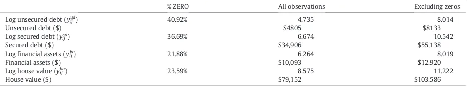
The sample of households analysed in this study forms a balanced panel where the same heads of household are observed in each wave yielding total observations over the period of 3930.4_{Table 1}_{provides summary statistics for the dependent variables.}_{Fig. 1} presents histograms of the natural logarithm of each dependent variable (see left hand side for the sample of all households). The right hand column ofFig. 1shows the distribution of each respective dependent variable excluding zeros. 41% (37%) of households over the period have no unsecured (secured) debt, with mean (median) values conditional on non-zeros being $8133 ($3125) and $55,138 ($43,529) for unsecured and secured debt, respectively. In terms offinancial assets, 22% (24%) of households have nofinancial assets (housing assets), with mean (median) values conditional on possessing such assets being $12,920 ($3497) and $103,586 ($79,096) forfinancial assets and house value, respectively.

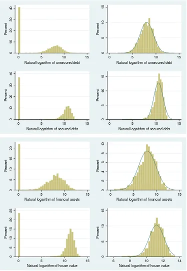
Fig. 2shows how the distribution of each dependent variable has changed between 1984 and 2011 conditional on positive amounts being held of each respective dependent variable. For unsecured debt, secured debt and house value, there has been a clear shift in the distribution to the right hand side, i.e. conditional on positive amounts being held, the average amount held has

(10)

increased and this is driven by higher amounts being held above the mean. This is less apparent for non-housing assets, where the distribution looks similar over time: although the mean amount held has increased between 1984 and 2011 from 7.8 to 8.2 log points ($7200 to $13,572), the tails of the distribution are similar. What underlies the distributions over time forfinancial assets is that a high proportion of the sample held non-housing assets in both 1984 and 2011, at 71% and 77%, respectively. Givenfinancial assets include checking and savings accounts, thesefigures are perhaps not surprising since such accounts are common being relatively low risk and highly liquid. For the other dependent variables, there are marked differences over time in the proportion of household holdings, where the correspondingfigures for those holding unsecured debt, secured debt and housing in 1984 (2011) are: 56% (65%); 45% (61%); and 46% (79%), respectively.

The independent variables used in the analysis to explain both the continuous parts and binary components of household debt and ﬁnancial asset holding, i.e.yi jqandpi jq, respectively (seeSection 2) whereq=ud,sd,fa,ha, follow the existing literature and consist of time invariant head of household characteristics and time varying variables. We also allow for full dynamics in both continuous and binary outcomes, by the inclusion of lagged dependent variablesyi jq−1andpi jq−1(seeSection 2). Time invariant variables are binary controls for: gender and ethnicity.

Time varying binary controls include age, specifically whether aged 18–24, aged 25–34, aged 35–44, aged 45–54 and aged 55–60 (where aged over 60 is the reference category). Other time varying controls include: marital status; whether the individual is in good or excellent health; employment status; whether the household is in the 0–25th income quartile; whether the household is in the 25– 50th income quartile; and whether the household is in the 50–75th income quartile (where above the 75th quartile is the reference category). We also control for the level of highest educational attainment of the head of family, which is defined as: not completed high school but more than eighth grade; completed high school; some college education; and a college degree or above (where below eighth grade is the reference category). Summary statistics and full definitions of the explanatory variables are given inTable 2.

In the four binary parts of the model,pi jq, i.e. the decision to hold a particular type of debt or asset, as inBrown et al. (2013), we include a set of additional variables. Specifically, we also include the proportion of household heads employed in thefinancial services in the state (this followsBertaut and Starr-McCluer, 2002), whether the head of household has been bankrupt in the past and the de-gree of risk tolerance of the head of household, which is increasing in risk tolerance.5_{In terms of modelling the level of unsecured debt,} yijud, andfinancial assets,yijfa, we also condition on whether the head of household has a mortgage.

4.2. Results

Table 3presents thefindings from applying the model detailed above to the PSID data whilstTable 4tests different model spec-ifications specifically: model 1, the joint model with dynamics (as detailed inSections 2 and 3above); model 2, the joint model with no dynamics, i.e. a static version of the model inSections 2 and 3; model 3, a joint model with dynamics but without exclusion restrictions (which are used to identify the binary outcomes); and model 4, which is characterised by independence, i.e._Σ= 0. Clearly, model 1 is the favoured specification since it has the smallest DIC and largest LPML. Hence, we can reject the null hypothesis that the preferred functional form is static. Such afinding is arguably unsurprising: we would predict the existence of state dependence in household_finances with respect to asset and debt holding. For example, secured debt holding is a relatively long-term commitment made by households.6

[image:10.544.42.508.74.161.2]

In terms of the set of additional variables used to model the probability of holding unsecured debt, secured debt,ﬁnancial assets and home ownership, these are jointly signiﬁcant in determining the decision to hold each item on the household balance sheet (seeTable 3). Moreover, the full joint dynamic model with the additional variables in the binary part (model 1) dominates the Table 1

Summary statistics for dependent variables.

% ZERO All observations Excluding zeros

Log unsecured debt (yijud) 40.92% 4.735 8.014

Unsecured debt ($) $4805 $8133

Log secured debt (yijsd) 36.69% 6.674 10.542

Secured debt ($) $34,906 $55,138

Logﬁnancial assets (yijfa) 21.88% 6.264 8.019

Financial assets ($) $10,093 $12,920

Log house value (yijha) 23.59% 8.575 11.222

House value ($) $79,152 $103,586

5_{In the 1996 PSID, a Risk Aversion Section was included containing detailed information on attitudes toward risk. This section of the PSID contains}_ﬁ_{ve questions} related to hypothetical gambles with respect to lifetime income. Hence, it is possible to rank individuals based on an ordinal index of risk attitudes.Kimball et al.

(2008, 2009)discuss some the disadvantages of this ordinal measure and alternatively assign a range of risk tolerance coefﬁcients to each gamble response category.

They argue that the imputations offer advantages over the categorical sequence of gamble responses in that the responses can be formulated into a single cardinal mea-sure of preferences. It is this cardinal risk tolerance meamea-sure which we adopt herein.

6

We have also performed prior sensitivity analysis. This was based on making various choices of prior parameters by changing only one parameter at a time and keeping all other parameters constant to their default values. This follows the standard practice in the Bayesian paradigm (see, for example,Ghosh and Gönen

(2008),Gelman et al. (2013), andStroud and Johannes (2014)). The main justiﬁcation behind this approach is that, with so many parameters, if the hyperprior values

(11)

corresponding model without such additional variables (model 3) in terms of the DIC and LPML statistics (seeTable 4). Hence, the null hypothesis that the additional variables included in the binary outcomes are jointly equal to zero is rejected.

Interestingly, heads of household who have been declared bankrupt in the past have a higher (lower) probability of holding un-secured (un-secured) debt, as found byBrown et al. (2013). Given that debt repayments are generallyﬁnanced from household income, it is apparent that if income is subject to risk (due to, for example, redundancy, unemployment, or changes in real wages), then the attitudes towards risk of the individual will potentially in_ﬂuence the decision to acquire debt, given the distribution of future income

0

10

20

30

40

Percent

0 5 10 15

Natural logarithm of unsecured debt

0

5

10

15

Percent

0 5 10 15

Natural logarithm of unsecured debt

0

10

20

30

40

Percent

0 5 10 15

Natural logarithm of secured debt

0

5

10

15

Percent

0 5 10 15

Natural logarithm of secured debt

0

5

10

15

20

Percent

0 5 10 15

Natural logarithm of financial assets

0

2

4

6

8

10

Percent

0 5 10 15

Natural logarithm of financial assets

0

5

10

15

20

25

Percent

0 5 10 15

Natural logarithm of house value

0

5

10

15

Percent

6 8 10 12 14

[image:11.544.84.458.50.593.2]

Natural logarithm of house value

(12)

and interest rates. In terms of the existing literature,Donkers and Van Soest (1999)find that risk averse Dutch homeowners tend to live in houses with lower mortgages, whilstBrown et al. (2013)report that risk aversion is negatively associated with the level of both unsecured and secured debt held. Our analysis sheds further light on the relationship between risk preference and householdfinances, in particular revealing that it is the decision to hold debt which is influenced by risk attitudes. To be specific, those heads of households who are more risk tolerant have a higher probability of holding unsecured and secured debt. As found byBertaut and Starr-McCluer (2002), the share of household heads employed in thefinancial services sector by state has a positive association with the probability of owning non-housingfinancial assets.

In terms of the dynamics, there is clear evidence of state dependence for both the continuous and binary parts of unsecured debt and house value, whilst dynamics only appear to be important (in terms of statistical signiﬁcance) for the binary parts of secured debt

0

.05

.1

.15

.2

.25

2 4 6 8 10 12

Log Unsecured Debt

1984

0

.1

.2

.3

.4

.5

6 8 10 12 14

Log Secured Debt

1984

0

.05

.1

.15

.2

.25

0 5 10 15

Log Financial Assets

1984

0

.2

.4

.6

6 8 10 12 14

Log House Value

1984

2011 2011

[image:12.544.97.454.51.312.2]

2011 2011

Fig. 2.Distributions of unsecured debt, secured debt,ﬁnancial assets and house value over time; conditional on positive values.

Table 2

Summary statistics of explanatory variables.

Variable Description Mean Standard deviation

Male =1 if male, 0 = female 0.4351 0.4958

Non-white =1 if non-white, 0 = other ethnicity 0.3257 0.4687

Married or cohabiting =1 if married or cohabiting, 0 = otherwise 0.8001 0.4002

Number of adults in household Number of adults (16+) in household 2.2695 0.7995

Number of kids in household Number of children (agedb16) in household 1.4018 1.1744 Excellent or good health =1 if in good/excellent health, 0 = poor/average 0.6336 0.4819

Employee =1 if employee, 0 = otherwise 0.8346 0.3716

Income in 0–24th percentile =1 if income in 0–25 percentile, 0 = otherwise 0.1295 0.3358 Income in 25–49th percentile =1 if income in 25–50 percentile, 0 = otherwise 0.2028 0.4021 Income in 50–75th percentile =1 if income in 50–75 percentile, 0 = otherwise 0.2969 0.4570

Aged 18–24 =1 if aged 18–24, 0 = otherwise 0.0493 0.2167

Did not complete high school =1 if not completed high school, 0 = otherwise 0.0331 0.1789

Completed high school =1 if completed high school, 0 = otherwise 0.3656 0.4817

Some college =1 if some college, 0 = otherwise 0.2585 0.4379

Graduated =1 if graduated, 0 = otherwise 0.3165 0.4652

Ever bankrupt =1 if previously bankrupt, 0 = otherwise 0.0789 0.2696

Risk tolerance Risk tolerance (higher values denote greater risk tolerance) 1.0678 2.1041 % inﬁnancial services by state Proportion of employed in theﬁnancial services in the state 0.0442 0.0355

[image:12.544.41.508.470.690.2]

(13)

andﬁnancial assets. In particular, focusing on unsecured debt, if the head of household held unsecured debt in the previous period then the probability of holding unsecured debt increases by 126 percentage points, ceteris paribus. However, the log amount of unsecured debt, conditional on holding a non-zero value, is decreasing in the amount held in the previous period. This might suggest that over time households are paying off such loans. In terms of house value, having housing equity in the previous period increases the probability of home ownership (either outright or on a mortgage) by 76 percentage points, ceteris paribus, and the current house value is a positive function of the value in the previous time period.

[image:13.544.44.503.73.407.2]

The importance of modelling both sides of the household balance sheet as a two-part process is apparent, as can be seen from

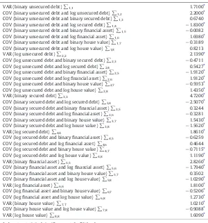
Table 4, since the diagnostic statistics reject the hypothesis that_Σ= 0. This can be seen by comparing the DIC and LPML from model 1 to that of model 4. Furthermore, it is clear fromTable 5that many of the variance and covariance terms inΣare statistically significant suggesting complex interactions across the various aspects of householdfinances. The interrelationship between household assets and liabilities is likely to be complicated. For example,Kullmann and Siegel (2005)show that exposure to real estate risk reduces householdfinancial asset holding, yet homeowners are more prone to invest in riskyfinancial assets such as shares traded in the stock market. The variance–covariance matrix of the errors terms,Σ, sheds some light on this: where statistically significant, correlations in the error terms suggest that there are unobserved factors which influence the probability of jointly holding different types of liabilities and assets. In accordance with thefindings ofKullmann and Siegel (2005), wefind evidence of statistically significant covariance terms between non-housingfinancial assets, such as stocks and shares, and home ownership.

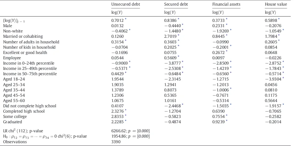
Table 3

Estimated Bayesian marginal effects (posterior means) of the independent variables upon binary and continuous outcomes.

Unsecured debt Secured debt Financial assets House value

prob(YN0) log(Y)|YN0 prob(YN0) log(Y)|YN0 prob(YN0) log(Y)|YN0 prob(YN0) log(Y)|YN0

{YN0}j−1 1.256⁎ – 2.176⁎ – 1.322⁎ – 0.755⁎ –

{log(Y)|YN0}j−1 – −0.474⁎ – −0.272 – 0.263 – 3.030⁎

Male −2.860⁎ 0.806⁎ −0.734⁎ −0.547 −0.142 0.738⁎ 0.043 0.061

Non-white −0.047 −1.102 0.550 −0.538 −0.561 −1.202⁎ −0.084 −0.492

Married or cohabiting −1.747⁎ 0.610 2.898⁎ 2.137⁎ 0.633⁎ 0.569 0.558⁎ 2.050⁎

Number of adults in household 1.290⁎ 0.131 0.144 0.275 −0.354⁎ 0.158 0.173⁎ 0.628⁎ Number of kids in household 1.092⁎ −0.371⁎ 0.451⁎ 0.474 −0.959⁎ −0.394⁎ 0.272⁎ 0.401⁎

Excellent or good health 0.088 −0.522⁎ 0.066⁎ 0.382 0.997⁎ 0.542⁎ 0.077 0.478⁎

Employee 2.085⁎ −0.121 0.302 0.603 −0.348 −0.088 0.281⁎ 0.277

Income in 0–24th percentile 3.515⁎ −1.484⁎ −1.712⁎ −2.042 −1.302 −1.502⁎ −0.760⁎ −1.636⁎ Income in 25–49th percentile 0.302 −1.290⁎ −1.778⁎ −1.576 0.152 −1.332⁎ −0.833⁎ −1.063⁎ Income in 50–75th percentile 3.636⁎ −0.224 −0.244 −0.715 0.938⁎ −0.254 −0.414⁎ −0.798⁎

Aged 18–24 −3.490⁎ 2.617⁎ −3.299⁎ −0.135 −2.177⁎ 2.466⁎ −1.853⁎ −0.289

Aged 25–34 −3.455⁎ 3.071⁎ −1.240 2.015⁎ −0.275 2.964⁎ −1.327⁎ 0.968

Aged 35–44 −2.541⁎ 2.783⁎ 0.167 2.817⁎ 0.737 2.679⁎ −0.340 2.043⁎

Aged 45–54 −0.866 1.947⁎ −0.131 2.540⁎ 0.284 1.785⁎ 0.384 1.970⁎

Aged 55–60 1.857⁎ 0.902 −0.250 2.608⁎ −0.085 0.832 0.546 2.320⁎

Did not complete high school −0.399 0.885 −0.285 1.115 0.801⁎ 0.946 0.618 1.598⁎

Completed high school 0.821 0.919 −1.349⁎ 0.212 1.203⁎ 0.965⁎ 0.196 0.989

Some college 3.713⁎ 1.430⁎ −0.692⁎ 0.556 0.571 1.509⁎ 0.373 1.579⁎

Graduated 3.761⁎ 1.702⁎ 1.812⁎ 0.628 0.725⁎ 1.820⁎ −0.289 0.894

Ever bankrupt 3.319⁎ – −1.043⁎ – 0.108 – 0.408 –

Risk tolerance 2.457⁎ – 1.327⁎ – −0.171⁎ – 0.097⁎ –

% inﬁnancial services by state −0.822 – −2.044 – 4.436⁎ – −1.947 –

No mortgage held 0.053 −0.140 – – −0.085 −0.272 – –

1989 −0.624 1.720⁎ 0.053 1.400⁎ −0.226 1.565⁎ 0.260 1.539⁎

1994 −1.462⁎ 1.345⁎ 0.699 1.880⁎ −0.298 1.205⁎ 0.404 2.414⁎

1999 1.934⁎ 1.077⁎ −0.613 1.271⁎ −1.212⁎ 0.934⁎ −0.506 1.890⁎

2001 −2.807⁎ 1.898⁎ −0.402 1.005 3.143⁎ 1.745⁎ −0.496 1.986⁎

2003 0.864 1.991⁎ −0.335 1.420⁎ 1.817⁎ 1.840⁎ 0.075 2.657⁎

2005 2.353⁎ 2.555⁎ 0.057 1.563⁎ 1.779⁎ 2.389⁎ −0.590 2.426⁎

2007 −2.859⁎ 2.214⁎ 0.656 2.053⁎ −0.628 2.079⁎ −0.395 2.781⁎

2009 0.979 2.696⁎ 0.558 2.538⁎ −0.429 2.535⁎ −0.372 3.059⁎

2011 −5.231⁎ 2.796⁎ 0.567 2.570⁎ 1.263⁎ 2.650⁎ −0.258 3.115⁎

Observations 3390

[image:13.544.36.499.635.689.2]

⁎ denotes statistical signiﬁcance at the 5% level.

Table 4 Model selection.

Model DIC LPML

1. Joint model with dynamics 1011.422 −0.4676

2. Joint model with no dynamics, i.e. static 1067.297 −0.6190

3. Joint model with dynamics and exclusion restrictions 1231.103 −0.6320

(14)

In addition to capturing relationships across the holding of the different types of debt and assets, the_flexibility of the two-part process is also evident when comparing the influence of the explanatory variables across the binary and the continuous parts of the model, where it can be seen that some explanatory variables exert different influences across these two parts (seeTable 3).

For example, it is apparent from the logistic model results that having a male head of household is inversely associated with the probability of holding unsecured debt yet exerts a statistically significant positive influence on, conditional on holding unsecured debt, the amount of unsecured debt held. As expected, having a married head of household has a very strong positive association with the probability of holding secured debt and a positive influence on the amount of secured debt held. Suchfindings may reflect the joint holding of debt within couples, such as a jointly held mortgage for the family home. On the opposite side of the household balance sheet, having a married head of household increases the probability of home ownership by 56 percentage points and has a positive influence on the amount of equity held where married individuals have approximately twice the amount of housing assets compared to single heads of household (conditional on home ownership).

Household composition is associated with householdﬁnances. This is particularly the case for unsecured debt, where a one standard deviation increase in the number of children in the household increases the probability of holding this type of debt by around 109 percentage points, yet conditional on holding unsecured debt, the number of children decreases the amount of debt held. The number of adults in the household, on the other hand, only inﬂuences the likelihood of holding unsecured debt.

[image:14.544.124.424.71.392.2]

With respect to the influence of health, the existing literature (see, for example,Bridges and Disney (2010), andJenkins et al. (2008)) generally supports a positive association between being in poor health and debt, although the direction of causality remains an unresolved issue here. Such a relationship may reflect an individual's inability to work whilst in poor health or may reflect direct costs associated with being in poor health such as additional transport costs or costs associated with medical care. Our results suggest that a head of household in poor health holds higher levels of unsecured debt compared to those in good or excellent health. Having a head of household in good health is positively associated with the probability of holdingfinancial assets, and, conditional on holding such assets, such individuals have around a 54 percentage points higher amount than a head of household in poor health. Such findings accord with thefinding of a positive association between unsecured debt and poor health in the existing literature, in that those individuals in poor health may facefinancial constraints and pressures and, as such, individuals in poor health may be less likely to holdfinancial assets. Ourfindings also tie in with those ofRosen and Wu (2004), who, using data from the U.S. Health and

Table 5

Variance–covariance matrix.

VAR (binary unsecured debt)∑1,1 1.7100⁎

COV (binary unsecured debt and log unsecured debt)∑1,2 2.2000⁎ COV (binary unsecured debt and binary secured debt)∑1,3 0.6740 COV (binary unsecured debt and log secured debt)∑1,4 −1.8300⁎ COV (binary unsecured debt and binaryﬁnancial asset)∑1,5 −0.0082 COV (binary unsecured debt and logﬁnancial asset)∑1,6 1.6980⁎ COV (binary unsecured debt and binary house value)∑1,7 −0.3189 COV (binary unsecured debt and log house value)∑1,8 0.8213

VAR (log unsecured debt)∑2,2 2.1390⁎

COV (log unsecured debt and binary secured debt)∑2,3 −0.4711 COV (log unsecured debt and log secured debt)∑2,4 0.5427⁎ COV (log unsecured debt and binaryﬁnancial asset)∑2,5 −1.9120⁎ COV (log unsecured debt and logﬁnancial asset)∑2,6 1.9120⁎ COV (log unsecured debt and binary house value)∑2,7 −0.5953⁎ COV (log unsecured debt and log house value)∑2,8 1.4350⁎

VAR (binary secured debt)∑3,3 4.7200⁎

COV (binary secured debt and log secured debt)∑3,4 −2.5070⁎ COV (binary secured debt and binaryﬁnancial asset)∑3,5 0.3244 COV (binary secured debt and logﬁnancial asset)∑3,6 −0.3281 COV (binary secured debt and binary house value)∑3,7 1.5430⁎ COV (binary secured debt and log house value)∑3,8 −1.5620⁎

VAR (log secured debt)∑4,4 1.8610⁎

COV (log secured debt and binaryﬁnancial asset)∑4,5 −0.6259 COV (log secured debt and logﬁnancial asset)∑4,6 0.4644 COV (log secured debt and binary house value)∑4,7 −0.7115⁎ COV (log secured debt and log house value)∑4,8 1.1190⁎

VAR (binaryﬁnancial asset)∑5,5 2.8260⁎

COV (binaryfinancial asset and logfinancial asset)∑5,6 −1.7940⁎ COV (binaryfinancial asset and binary house value)∑5,7 0.3502 COV (binaryfinancial asset and log house value)∑5,8 −1.0290⁎

VAR (logﬁnancial asset)∑6,6 1.8100⁎

COV (logﬁnancial asset and binary house value)∑6,7 −0.5206⁎ COV (logﬁnancial asset and log house value)∑6,8 1.2730⁎

VAR (binary house value)∑7,7 1.0210⁎

COV (binary house value and log house value)∑7,8 −0.9088⁎

VAR (log house value)∑8,8 1.6090⁎

(15)

Retirement Survey,ﬁnd that being in poor health is inversely associated with the probability of holding a range ofﬁnancial assets in-cluding bonds and risky assets such as stocks and shares.

With respect to economic andfinancial factors, having a head of household in employment is positively associated with holding unsecured debt, with employees being twice as likely to hold unsecured debt compared to those not in employment. However, conditional on holding this type of debt, employment does not appear to in_fluence the amount of unsecured debt held. Such afinding ties in with our a priori expectations in that being employed is often a prerequisite for taking out a personal loan or a credit card. The only other instance of where labour market status has a statistically significant effect in the two-part model is on the probability of home ownership where employed heads of household are 28 percentage points more likely to own their home.

The three household income quartile controls are all inversely associated with the probability of holding secured debt relative to being in the top household income quartile and statistically significant (with the exception of those above the median). This inverse association is also apparent in the continuous part of the model but does not reach levels of statistical significance. Such results reinforce thefindings in the existing literature related to a positive association between income and secured debt. Worryingly, focusing on the probability of holding unsecured debt, those in the bottom income quartile are 3.5 times more likely to hold such debt compared to those households in the top part of the income distribution. Turning to the opposite side of the household balance sheet, there is a monotonic relationship between household income and the amount offinancial assets (conditional on holding financial assets) and the amount of housing assets (conditional on owning a home).

Interestingly, the results suggest that the age of the head of household has a statistically signi_ficant negative in_fluence on the probability of holding unsecured debt yet statistically significant positive effects on the amount of unsecured debt are apparent for all age groups relative to individuals aged over 60. The age effects peak for those aged 25 to 34 who have approximately three times the amount of unsecured debt than those aged over 60. Such age effects may reflect consumption smoothing over the life cycle, with individuals aged between 25 and 54 being engaged in activities such as marriage, bringing-up children or house buying at various stages of the life cycle, when consumption may exceed income for a variety of such reasons. As individuals become older, debt levels typically fall as loans are repaid and/or as income increases, which is in accordance with the signs of the estimated coefficients. In contrast to the striking association between age and unsecured debt, there are generally no effects from age on the probability of holding secured debt. The exception to this is those heads of household aged 18 to 24 who are more than three times less likely to hold mortgage debt than those aged above 60. However, age effects are apparent when focusing on the amount of secured debt held, conditional on holding such debt, where again life cycle factors would appear to matter with the level of debt culminating when aged 35 to 44.

Focusing on the role of age effects on the opposite side of the household balance sheet, age effects are not apparent in the binary part of the model forfinancial assets or housing assets yet all age groups have a positive influence on the amount offinancial assets held relative to the aged over 60 group, with the size of the effect declining across the age groups.7_{For example, those aged 25 to} 34 have approximately three times the value offinancial assets compared to those aged above 60. Suchfindings, which tie in with the concave relationship found between age and the holding of stocks and shares in the existing literature, see for exampleShum and Faig (2006), may once again be capturing life cycle effects and may, for example, reflect dis-saving associated with retirement as older individuals move out of the labour market and liquidatefinancial assets in order to supplement their pension income.

With respect to the educational attainment of the head of household, the two highest levels of educational attainment, namely having some college education and college education and above are both positively related to the probability of holding unsecured debt relative to having below eighth grade school education. For example, a head of household who has college education and above is nearly four times more likely to hold unsecured debt than those whose highest level of education is below eighth grade. With respect to the amount of unsecured debt held, conditional on holding this type of debt, a head of household who has graduated holds 170 percentage points more unsecured debt relative to heads having below eighth grade education. Turning to secured debt, the only effect that educational attainment has is on the probability of holding mortgage debt. For example, a head of household who has graduated has a 181 percentage point higher probability of holding such debt compared to those with education below eighth grade, i.e. being nearly two and half times as likely to hold such debt. Moreover, there is no signiﬁcant impact from education on the level of secured debt. Thus, the differences in theﬁndings related to educational attainment across the binary and the continuous parts of the framework highlight the importance of applying the two-part modelling approach and may explain the mixed results relating to the relationship between education and debt reported in the existing literature, see, for example,Brown and Taylor (2008).

Turning tofinancial assets and the role of educational attainment, no clear pattern emerges other than that those who have graduated have a higher probability of holding non-housingfinancial assets and, conditional on ownership of such assets, they hold larger amounts: specifically 182 percentage points more than those with education below eighth grade, ceteris paribus. This again concurs with the existing literature, see, for exampleHong et al. (2004)for the U.S. andGuiso et al. (2008)who analyse Dutch and Italian survey data.

Controls for the year of interview are incorporated into the analysis in order to account for unobserved macroeconomic conditions that have the potential to affect all households. Interestingly, the value of each type of debt conditional on holding that type of debt has generally increased over time compared to the base year of 1984. This is especially the case post 2001 for unsecured and secured debt. This is an effect over and above in_ﬂation since monetary values are held at constant prices.