Evaluation of FSK models for radiative heat transfer under oxyfuel conditions

(1)

This is a repository copy of Evaluation of FSK models for radiative heat transfer under oxyfuel conditions.

White Rose Research Online URL for this paper: http://eprints.whiterose.ac.uk/89151/

Version: Accepted Version

Article:

Clements, A.G. orcid.org/0000-0003-3778-2248, Porter, R., Pranzitelli, A. et al. (1 more author) (2015) Evaluation of FSK models for radiative heat transfer under oxyfuel

conditions. Journal of Quantitative Spectroscopy and Radiative Transfer, 151. pp. 67-75. ISSN 0022-4073

https://doi.org/10.1016/j.jqsrt.2014.09.019

Article available under the terms of the CC-BY-NC-ND licence (https://creativecommons.org/licenses/by-nc-nd/4.0/).

Reuse

This article is distributed under the terms of the Creative Commons Attribution-NonCommercial-NoDerivs (CC BY-NC-ND) licence. This licence only allows you to download this work and share it with others as long as you credit the authors, but you can’t change the article in any way or use it commercially. More

information and the full terms of the licence here: https://creativecommons.org/licenses/

Takedown

If you consider content in White Rose Research Online to be in breach of UK law, please notify us by

(2)

Evaluation of FSK models for radiative heat transfer

under oxyfuel conditions

Alastair G. Clementsa,∗

, Rachael Porter, Alessandro Pranzitellia_,

Mohamed Pourkashaniana

a

Energy Technology and Innovation Initiative, University of Leeds, Leeds, LS2 9JT, UK

Abstract

Oxyfuel is a promising technology for carbon capture and storage (CCS)

applied to combustion processes. It would be highly advantageous in the

de-ployment of CCS to be able to model and optimise oxyfuel combustion,

how-ever the increased concentrations of CO2 and H2O under oxyfuel conditions

modify several fundamental processes of combustion, including radiative heat

transfer. This study uses benchmark narrow band radiation models to

evalu-ate the influence of assumptions in global full-spectrum k-distribution (FSK)

models, and whether they are suitable for modelling radiation in

computa-tional fluid dynamics (CFD) calculations of oxyfuel combustion. The

statist-ical narrow band (SNB) and correlated-k (CK) models are used to calculate

benchmark data for the radiative source term and heat flux, which are then

compared to the results calculated from FSK models. Both the full-spectrum

correlated k (FSCK) and the full-spectrum scaled k (FSSK) models are

ap-plied using up-to-date spectral data. The results show that the FSCK and

FSSK methods achieve good agreement in the test cases. The FSCK method

∗_{Corresponding author}

(3)

using a five-point Gauss quadrature scheme is recommended for CFD

calcu-lations in oxyfuel conditions, however there are still potential inaccuracies in

cases with very wide variations in the ratio between CO₂ and H₂O

concen-trations.

Keywords: Radiative transfer, Oxyfuel, Computational fluid dynamics, Full-spectrum k-distributions

1. Introduction

Oxyfuel is a promising technology to abate CO2 emissions from

combus-tion facilities. The process replaces air with high purity oxygen as the oxidant

for fuel combustion. The oxygen supply is often diluted with recycled flue

gas to control the flame temperature. The resulting flue gas from the oxyfuel

process is composed entirely of the products from combustion, with a very

high CO2 concentration that can be purified to a level suitable for storage.

Oxyfuel combustion has been successfully demonstrated at small scales [1–

3], and there are further projects in development aiming to demonstrate the

technology at much larger scales, such as the White Rose1_{, FutureGen 2.0}2

and Youngdong projects.

There are several changes to the fundamental properties of combustion

under oxyfuel, where the transparent and inert bulk gas N2 is replaced with

radiatively participating and potentially reactive CO₂ and H₂O.

Further-more, there are additional avenues of control available in the oxyfuel process,

as the gas composition of the inlets is completely defined by the operator.

1_{http://www.whiteroseccs.co.uk/}

(4)

Drying or cooling the flue gas recycle, or changing the oxygen enrichment

level, could result in drastic changes to the combustion process. In the

de-velopment of oxyfuel technology it would be extremely useful to be able to

accurately predict the influence of these changes to optimise the process,

however models developed for predicting air-fired combustion may not be

suitable for oxyfuel, with the models used for radiative heat transfer being

repeatedly identified as a key area of research for oxyfuel modelling [4–6].

Radiation is the most significant thermal transfer mechanism at

combus-tion temperatures. Failure to accurately account for the effects of thermal

radiation will significantly affect further modelling predictions such as heat

flux, gas velocity and species concentration predictions. The process of

radi-ative transfer is influenced by the medium, where participating species, such

as CO₂ and H₂O, will emit and absorb radiative energy. Accurate

consider-ation of gas-phase radiconsider-ation is important even in atmospheres where highly

emissive particles, such as soot, are present due to strong self-absorption [7].

Combustion modelling has often made use of the grey weighted sum of

grey gases (WSGG) method to account for gas absorption/emission in

ra-diative transfer. The grey WSGG model has been successfully applied to

air-fired combustion, but is only valid for predetermined environments, and

the traditional models are unable to predict key radiative quantities in an

oxyfuel environment [8, 9]. The full-spectrum k-distribution (FSK) models

offer an alternative approach to accurately calculate radiative heat transfer

for arbitrary gas mixtures, and can be evaluated fast enough to be applied in

complex computational fluid dynamics (CFD) calculations [9, 10]. Previous

(5)

CFD calculations, highlighting the need to accurately account for radiation

heat transfer [7, 11, 12]. In addition to the FSK models that are the focus of

this study, other global methods, such as the absorption distribution

func-tion (ADF) [13] and spectral line-based weighted sum of grey gasses (SLW)

[14], are also potentially viable for calculating radiative transfer in novel

en-vironments within CFD calculations. These additional global models have

been shown to be related to the FSK models [15, 16], and so the conclusions

of this study may also be applicable to the ADF and SLW models.

This work focusses on the application and validation of FSK models to

predict radiation heat transfer in oxyfuel environments within a

commer-cial CFD code. The FSK models are validated against narrow-band

predic-tions on a 3D enclosure that represents potential oxyfuel combustion

envir-onments. Calculations of the radiation energy source term and heat flux are

compared between the benchmark narrow-band models, the standard grey

WSGG model and the FSK models. A previous study identified FSK models

as being accurate in potential air and oxyfuel cases [9]; this study updates the

validation data and FSK parameters to recently developed spectral database

values, and validates both the spectrum correlated k (FSCK) and

full-spectrum scaled k (FSSK) models against two cases that test the underlying

assumptions in the models for non-isothermal and non-homogeneous media.

This study also identifies the optimal number of transfer equations that are

required for the FSK models in the identified cases. The WSGG and FSK

methods are implemented so that they are directly applicable to CFD

calcu-lations, allowing the conclusions from this study to be directly applicable to

(6)

2. Modelling radiative heat transfer

The directional radiative transfer equation (RTE) for an emitting,

ab-sorbing and non-scattering medium, assuming radiative equilibrium, is given

as

dIη

dˆs =κη(φ) Ibη−Iη

(1)

where η denotes wavenumber, Iη is the spectral radiative intensity, ˆs is a

ray direction through the medium, Ibη is the spectral blackbody intensity,

κη is the spectral absorption coefficient of the medium and φ is a vector of

the local gas properties that affect the absorption coefficient, namely

pres-sure, temperature and gas composition. This study focuses on methods that

evaluate the radiative intensity of a participating gas-phase medium, where

absorption and emission are significant and scattering effects are negligible,

so the RTE formulation in Equation (1) is adequate.

Radiation is coupled to the energy solution in CFD calculations through

the radiation source term and the radiative heat flux. The radiation source

term is the divergence of radiative heat flux through the medium, and can

be calculated from the radiation intensity field as

∇ ·qr =

Z ∞

0

κη(φ)

4πIbη− Z

4π

IηdΩ

dη (2)

where ∇ ·qr is the radiative source term, qr is the radiative heat flux at

a position in the domain and Ω denotes solid angle. The radiation source

term is important in calculating the temperature field, which has a

signi-ficant impact on fluid dynamics and chemical reaction rates. The radiative

contribution to the total heat flux at a surface can be calculated as

qr·nˆ =

Z ∞

0 Z

4π

(7)

where ˆn is the inward surface normal. Most of the surface heat flux in

com-bustion systems is due to radiation, making the accurate treatment of this

quantity important in evaluating the performance of the operating

paramet-ers for combustion.

Determining the quantities in Equations (2) and (3) across the whole

spectral dimension is computationally expensive due to the variability of

the absorption coefficient, which oscillates at very small spectral intervals –

the exhaustive line-by-line (LBL) method typically requires over 106 _RTE

evaluations. The behaviour of the absorption coefficient for a potential

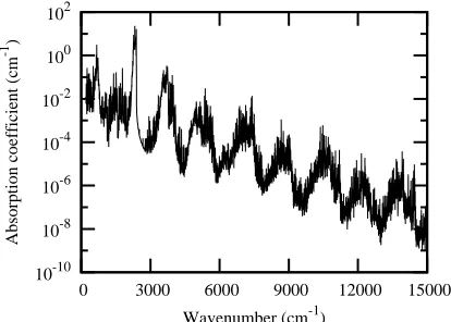
oxy-fuel environment is shown in Figure 1. This study uses statistical narrow

band (SNB) and correlated-k (CK) models to generate benchmark data to

validate the global FSK models, which are also compared to the more

stand-ard grey WSGG model.

The SNB model is able to reach LBL accuracy in special cases within

an acceptable time-frame, making it suitable for 3D calculations. The SNB

model is often used to generate data for validating more time-efficient and

widely-applicable models [9, 10, 17]. The CK model offers an alternative

source of benchmark data to the SNB model, and the model provides a more

amenable representation of absorption and emission, and is therefore

applic-able to more general RTE solvers. Global models, such as the WSGG and

FSK models, calculate spectrally integrated values directly, allowing the

solu-tion to radiative transfer to be coupled with complex numerical simulasolu-tions,

as in CFD calculations, which is not viable with narrow-band models. This

study validates the simplifying assumptions in the FSK models for oxyfuel

(8)

10-10 10-8 10-6 10-4 10-2 100 102

0 3000 6000 9000 12000 15000

Absorption coefficient (cm

-1 )

[image:8.595.201.408.130.278.2]

Wavenumber (cm-1)

Figure 1: Absorption coefficient for a gas mixture of 85% CO₂, 10% H₂O and 5% N₂ at

1000K. Calculated from HITEMP2010 [18].

2.1. The statistical narrow-band model

The SNB model calculates radiation transfer based on averaged values

across a narrow band, which are typically ∆η=25cm-1 _{wide. The SNB model}

provides values for averaged band transmittance based on a statistical

rep-resentation of the optical properties. For an isothermal and homogeneous

path between s and s′

, the Malkmus [19] SNB model that is used in this

study approximates the mean average transmittance across a narrow band

as

¯

τs→s′ = exp

  − 2¯γ ¯ δ   s

1 + ¯kδxpl¯ ¯

γ −1



 



 (4)

where ¯γ is the mean spectral line Lorentz half-width, ¯δ is the mean line

spacing, ¯k is the mean intensity-to-spacing ratio, x is the absorbing species

mole fraction,pis the pressure of the medium andlis the path length between

s and s′

.

(9)

transmittance, the discrete form of the narrow-band averaged RTE for black

walls is given as [20]

¯

I∆η = I¯w∆η¯τ∆η,1→_N+1 +

N X

i=1

¯

Ib∆η,i+1_/2 ¯τ∆η,i+1→_N+1−τ¯∆η,i→_N+1

(5)

where ¯I∆η is the narrow-band averaged intensity, ¯Ib∆η,i+1_/2 is the narrow-band

averaged blackbody intensity between pointiandi+1 along the path, ¯Iw∆ηis

the narrow-band averaged intensity emitted from the boundary, where i= 1,

and N is the number of discrete points along the path. The SNB model is

ill-suited for calculating radiative transfer in scattering media or for cases

with non-black walls, however in the cases that are considered in this study

the SNB model is accurate enough to produce results that can be considered

a very good representation of the radiation field.

This work used a ray-tracing approach similar to the method described

by Liu [17] to calculate the radiative source term and heat flux for a

three-dimensional enclosure. The radiative intensity at a control surface is

calcu-lated by tracing a number rays from the centre of the surface to the boundary,

and calculating the intensity propagating from the boundary back towards

the control surface, using Equation (5). Discrete segments of the rays are

defined as sections that are entirely inside one control volume, and were

con-sidered uniform with respect to the values calculated for the centre of the

control volume. Non-homogeneous and non-isothermal paths were calculated

using the Curtis-Godson approximation [21], which introduces a scaled

as-sumption across narrow-band intervals. The radiative source term, ∇ ·qr,

was calculated using a first-order finite difference scheme. The number and

(10)

sensitiv-ity of the solution to the angular quadrature set was tested by running the

calculation on increasing Tn sets until the solution was consistent with the

next two sets. This method was chosen as it accurately represents the RTE,

however it is noted that the implementation is not optimised for efficiency

[17].

2.2. The correlated-k model

The CK model calculates narrow-band intensity through a reordered

ab-sorption coefficient across the band. By transforming the RTE to be defined

as a function of a reordered distribution, which is chosen to be a smooth

increasing function, it is possible to calculate band-averaged quantities using

an efficient and accurate numerical quadrature scheme. The k-distribution

across a narrow-band, f(φ, k), is defined as

f(φ, k) = 1 ∆η

Z

∆η

δk−κ(φ)dη (6)

where δ is the Dirac delta function. The k-distribution represents the

fre-quency that the absorption coefficient takes on a certain value, which is

denoted ask in Equation (6). The narrow bands are chosen so that the

black-body intensity is practically constant across the band, so that its variations

can be neglected. By taking the cumulative function of the k-distribution,

defined as

g(φ, k) = Z k

0

f(φ, k′

) dk′

(7)

it is possible to describe the k-distributions with a function bound between

zero and one. The cumulative distribution g(φ, k) represents the fraction of

(11)

The RTE for narrow-band intensity using the CK model is presented as

d ¯I∆η,gi

dˆs =k∆η(φ, gi) Ibη0 −I¯∆η,gi

(8)

where ¯I∆η,gj is the band-averaged intensity at g-space value gj, Ibη0 is the

blackbody intensity evaluated at the band centre and k∆η(φ, gi) is the

re-ordered absorption coefficient in g-space, the inverse of the function shown

in Equation (7). Using a suitable quadrature scheme, the total intensity can

be evaluated as

Z ∞

0

Iηdη≈ Nb

X

n ∆ηn

Nq

X

i

wiIn,i (9)

where Nb is the number of spectral bands, Nq is the number of quadrature

points and wi is the quadrature weight associated with point i.

The reordering operation introduced in Equation (6) is not strictly valid

for different values of φ, and therefore the k-distribution method cannot be

applied to inhomogeneous media without a simplifying approximation of the

absorption coefficient. Introducing a correlated assumption for the

absorp-tion coefficient within a narrow band, the differences in k(φ, gj) between the

g-space dimension of different thermodynamic states are neglected [23]. The

introduction of the correlated assumption complements the scaled

assump-tion introduced to the SNB model with the Curtis-Godson approximaassump-tion.

In this work, the CK model parameters presented by Rivi`ere and Soufiani

[24] are used, which describe 51 narrow bands with a seven-point quadrature

scheme, resulting in 357 RTE evaluations. The mixing scheme by Modest

and Riazzi [25] is used to approximate k-distributions for gas mixtures from

the single-specie CK model parameters. As the CK model describes the

(12)

solver as the FSK methods.

2.3. Full-spectrum k-distribution models

Similarly to the CK model, the FSK models calculate total intensity with

a reordered absorption coefficient. The FSK model uses k-distributions across

the entire spectrum, which are weighted by the Planck function to account

for the variations in blackbody emissivity, as it can no longer be considered

constant,

f(φ, T, k) = 1

Ib(T) Z ∞

0

Ibη(T, η)δk−κ(φ)dη (10)

where f(φ, T, k) is the full-spectrum k-distribution,Ib is the total blackbody

intensity integrated across the spectrum and δ is the Dirac delta function.

To facilitate integration, the spectral dimension is normalised, and redefined

as the cumulative k-distribution at a reference state;

g0(T0, φ₀, k) = Z k

0

f(T0, φ₀, k

′

) dk′

(11)

whereg0 is the cumulative k-distribution at a reference stateφ₀and reference

temperature T0. As with the CK model, the reordering operation in

deriv-ing the full-spectrum k-distribution results in the spectral dimension of two

states not being directly related, and the absorption coefficient is required

to be treated as either scaled or correlated across the entire spectrum. This

treatment of the absorption coefficient is the main source of error in FSK

models [26].

As it was mentioned for the CK model, it can be shown that the

cumu-lative k-distribution for two correlated states is the same, and the RTE can

(13)

emitting and absorbing medium can be rewritten for the FSCK model as

dIg dˆs =k

∗

(T0, φ, g0)

a(T, T0, g0)Ib(T)−Ig

(12)

where

Ig = R∞

0 Iηδ(k−kη) dη

f(T0, φ₀, k)

(13)

a(T, T0, g0) =

f(T, φ₀, k)

f(T0, φ₀, k)

= dg(T, φ0, k)

dg0(T0, φ₀, k)

(14)

and where k∗

is the correlation function that relates the reference

cumulat-ive k-distribution to the local state. Due to the smooth k-g distribution,

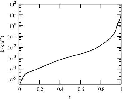
illustrated in Figure 2, the total radiative intensity can be integrated across

g-space using an efficient Gauss quadrature scheme [27],

Z ∞

0

Iηdη= Z 1

0

Igdg0 ≈

Nq

X

i

wiIgi (15)

where Nq is the number of quadrature points used in the integration, wi is

the Gauss quadrature weight associated with quadrature point i and Igi is

the intensity evaluated for quadrature point i.

Alternatively to the correlated assumption, the absorption coefficient

could be assumed to be scaled. The variation of a scaled absorption

coeffi-cient at different states can be separated from the spectral variation,

κ(η, φ) =κ(η, φ₀)u(φ₀, φ) (16)

whereu(φ₀, φ) is a scalar function. Using k-distributions, ucan be calculated

using the implicit relation [26]

Z 1

0

exph−k(T0, φ, g)s i

dg = Z 1

0

exph−k(T0, φ₀, g0)u(φ₀, φ)s i

(14)

10-5 10-4 10-3 10-2 10-1 100 101 102

0 0.2 0.4 0.6 0.8 1

k (cm

-1 )

[image:14.595.203.400.129.287.2]

g

Figure 2: Full-spectrum k-g distribution calculated from the absorption coefficient in

Figure 1.

where s is the mean beam length of the domain, which can be calculated

using a commonly used relation based on the geometry [23]. In this work

the mean beam length is calculated as s = 3.6V /A, where V is the internal

volume of the domain and A is the bounding surface area. The integrations

in Equation (17) can be evaluated using a Gauss quadrature scheme, and

the relation can be effectively solved for the scaling function u by using a

Newton-Raphson scheme [26]. Similarly to the FSCK model, the RTE for

the FSSK model can be written as

dIg

dˆs =k(T0, φ0, g0)u(φ0, φ)

a(T, T0, g0)Ib(T)−Ig

(18)

The total intensity for the FSSK model can also be calculated using

Equa-tion (15).

It is important to select a representative reference state and temperature

for the FSCK and FSSK models, as this is the only condition where both

(15)

T0 is also used for the reference stateφ₀, and is calculated using the implicit

relation [26]

κpl(φ

0)Ib(T0) =

1

V

Z

V

κpl(φ)I_b(T) dV (19)

where κpl(φ) is the Planck-function weighted mean absorption coefficient at

state φ. The mole fractions of the species for φ₀ are calculated as volume

weighted averages across the domain. The reference pressure is set to

atmo-spheric pressure as the cases in this study are all at constant atmoatmo-spheric

pressure.

The computational requirements of the FSCK and FSSK models are

nearly identical, with the FSSK model only requiring a small increase in

com-putational effort in the pre-processing step of calculating the scaling function

[26]. Although the scaling approximation appears more constrictive, previous

studies have shown that the predictions are often more accurate when the

absorption coefficient is poorly correlated as Equation (14) provides a way to

fit the k-distributions, which are truly neither scaled nor correlated, to the

case being studied [26]. The most time-consuming part of the FSK models for

CFD calculations is the number of RTEs that are required, which is dictated

by the number of quadrature points used in Equation (15). It is important

to choose the smallest number of points to ensure timely evaluation, while

not sacrificing too much accuracy in the solution.

The calculation of the k-distributions used in Equation (12) and the

scaling function in Equation (17) can be time-consuming to calculate from

line-by-line data. To avoid this overhead it is possible to calculate the

full-spectrum k-distributions for a gas mixture from narrow-band single-specie

(16)

full-spectrum k-distributions were calculated from a database generated by Cai

and Modest [28] that was updated for the HITEMP2010 data [18], and is

provided as part of the Spectral Radiation Calculation Software (SRCS). To

further reduce the computational effort, the k-distributions, scaling functions

andafunctions were calculated in a pre-processing step, generating a look-up

table for a series of predetermined values ofφandT, and linear interpolation

between these values was used when solving the RTE. The resolution of the

lookup table was set to similar values to the resolution of the database, and

increasing this resolution did not affect the solution. The mixing scheme by

Modest and Riazzi [25] is used in this study to calculate the k-distributions of

H₂O/CO₂ mixtures. The difference in the spectral data used to evaluate the

benchmark and FSK data for CO2 may introduce a source of error, however

these errors should be small at the temperatures being considered in this

study, which are below 2000K [29].

Both the correlated and scaled assumptions often break down in cases

with large gradients in temperature [30] or relative species concentrations

[27]. Under combustion conditions it is expected that there will be

signific-ant gradients in temperature at the flame edge, which could also coincide

with significant variations in relative species concentrations. Specifically for

oxyfuel, especially if the flue gas recycle is pre-dried, it is likely there will be

areas with a high CO₂ concentration juxtaposed to a reaction zone producing

a variable ratio of H2O and CO2. The approximations in the FSK models

need to be validated against possible oxyfuel conditions before they can be

(17)

3. Case descriptions

The test cases used in this study are similar to the cases previously

pro-posed by Liu [17]. The radiative source term, Equation (2), and

radiat-ive heat flux, Equation (3), are solved for a 2m×2m×4m enclosure, that is

bounded by black walls and contains a participating medium with a fixed

composition and temperature.

The first case is the same as the case proposed by Porter et al. [9]. The

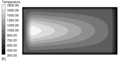
enclosure contains a gas mixture that is 85% CO₂, 10% H₂O and 5% N₂

by volume, with a temperature profile that is non-uniform but symmetric

around the centreline parallel to the z-axis. The centreline temperature is

a piecewise linear profile that increases from 400K at z=0m, to 1800K at

z=0.375m and then decreases to 800K at z=4m. The radial temperature

distribution is defined as

T =    

  

(Tc−800)f(r) + 800 r≤1

800 r >1

(20)

where Tc is the centreline temperature,r is the distance of the location from

the centreline and where f(r) = 1−3r2_{+ 2}_r3_{. The walls are kept at 300K.}

The temperature distribution is illustrated in Figure 3. The geometry is

di-vided into a 17×17×24 cell grid, with a higher density of cells in the high

temperature region, identical to the third case by Liu [17]. The SNB

bench-mark data in this work is updated with the new parameters from Rivi`ere

and Soufiani [24]. The T6 quadrature scheme was used to generate the SNB

benchmark data. Increasing the number of rays to the T8 scheme did not

(18)

[image:18.595.204.405.126.230.2]

Figure 3: The temperature distribution in the first case on the Y=1m plane.

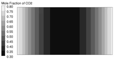
The second case is defined to represent a wide range of product species

ratios that may occur under oxyfuel conditions. The temperature is uniform

within the enclosure at 1500K, and the walls are black at 500K. The species

distribution within the enclosure is non-uniform and varies so that the molar

ratio of H₂O/CO₂ is bound between 0.125 and 2, with individual species

defined as

XH2O = 2

z

4 1−

z

4

+ 0.1 (21)

XCO2 = 0.9−XH2O (22)

XN2 = 0.1 (23)

where Xsp is the mole fraction of species sp. The distribution of the mole

fraction of CO2 is illustrated in Figure 4. CO radiation was not considered

in either case as the majority of the radiative heat flux and source term are

expected to arise from interactions from CO2 and H2O, especially in oxyfuel

cases with recycled flue gas. For the second case the geometry was divided

into a uniform 11×11×25 cell grid. The T8 quadrature scheme was used

for the SNB results on the second case as there were noticeable differences

(19)

[image:19.595.204.404.123.227.2]

Figure 4: The CO₂ distribution in the second case on the Y=1m plane.

Each solution was obtained using the commercial CFD code ANSYS

Flu-ent v14.5, incorporating user-defined functions to customise the radiation

model. The benchmark SNB data were calculated within ANSYS Fluent

v14.5 using an ‘on-demand’ user-defined function to ensure that the geometry

was identical between the narrow-band and global models. The finite volume

method (discrete ordinates) provided in ANSYS Fluent was used to calculate

the CK model results, using an angular discretisation of Nθ = Nφ = 3.

In-creasing the angular discretisation to Nθ =Nφ= 4 did not alter the results.

Due to the reasonably large spacial resolution, producing a relatively

sig-nificant optical thickness for each control volume, the second-order upwind

method was used to calculate control surface values.

For both cases, the FSCK and FSSK models were evaluated using a

Gauss quadrature scheme, where the number of quadrature points were

var-ied between three and nine, and were applvar-ied using the same finite volume

method to solve the RTE as described with the CK model. For brevity, only

the results for three, five and seven quadrature points in the FSK models are

shown, as the solution did not change significantly for more than five points.

(20)

were run in serial on a 3 GHz CPU and took less than a couple of minutes to

reach a converged solution for the FSK models, however there was a

notice-able time penalty when applying a higher number of quadrature points. The

results from the FSK models are also compared against the results from the

grey WSGG model that is available in ANSYS Fluent v14.5, which is based

on the coefficients by Smith et al. [31].

4. Results and discussion

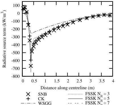
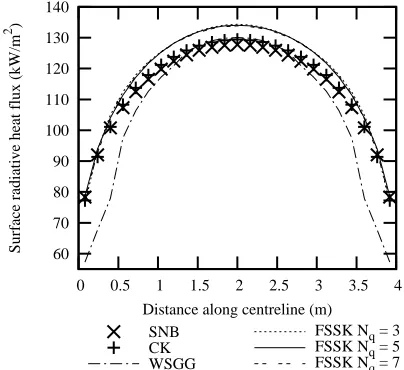
The results for the first case are shown in Figures 5 and 6, illustrating the

variation of the radiative source term along the centreline parallel to the

z-axis and the surface radiative heat flux on the wall along the line (0m,1m,z).

The results show that an optimal choice for the number of quadrature points

lies around five points, as there is only a small change in the derived values

as this number increases. The results of the SNB and CK models show a

disagreement in peak regions.

Both of the FSK models demonstrate similar predictions for the radiative

source term in the first case, with the FSCK and FSSK models (Figures 5a

and 6a respectively) marginally under-predicting the magnitude of the source

term with respect to the benchmark data. The FSCK and FSSK models also

produce very similar results with regards to the radiative surface heat flux,

shown in Figures 5b and 6b, over-predicting the values calculated with the

narrow-band models. The very good agreement between the FSK models

and the CK model supports the assessment that the discrepency between the

benchmark data can be attributed to the different RTE solvers, and that the

(21)

-800 -700 -600 -500 -400 -300 -200 -100 0 100

0 0.5 1 1.5 2 2.5 3 3.5 4

Radiative source term (kW/m

3 )

Distance along centreline (m) SNB

CK WSGG

FSCK N_q = 3 FSCK N_q = 5 FSCK N_q = 7

(a) Radiative source term calculations along the

centreline.

6 8 10 12 14 16 18 20 22

0 0.5 1 1.5 2 2.5 3 3.5 4

Surface radiative heat flux (kW/m

2 )

CK WSGG

(b) Surface radiative heat flux calculations along

[image:21.595.199.403.133.316.2]

the wall line (0m,1m,z).

(22)

-800 -700 -600 -500 -400 -300 -200 -100 0 100

0 0.5 1 1.5 2 2.5 3 3.5 4

3 )

CK WSGG

FSSK N_q = 3 FSSK N_q = 5 FSSK N_q = 7

centreline.

6 8 10 12 14 16 18 20 22

0 0.5 1 1.5 2 2.5 3 3.5 4

2 )

CK WSGG

[image:22.595.199.403.133.317.2]

(23)

-300 -250 -200 -150 -100

0 0.5 1 1.5 2 2.5 3 3.5 4

3 )

CK WSGG

centreline.

60 70 80 90 100 110 120 130 140

0 0.5 1 1.5 2 2.5 3 3.5 4

2 )

CK WSGG

[image:23.595.200.401.130.317.2]

(24)

-300 -250 -200 -150 -100

0 0.5 1 1.5 2 2.5 3 3.5 4

3 )

CK WSGG

centreline.

60 70 80 90 100 110 120 130 140

0 0.5 1 1.5 2 2.5 3 3.5 4

2 )

CK WSGG

[image:24.595.199.401.381.566.2]

(25)

In contrast to the FSK models, the predictions from the WSGG method

show significant disagreement with the benchmark data, as was reported

previously by Porter et al. [9].

The results for the second case are illustrated in Figures 7 and 8. As with

the first case, the plots represent the calculated values for radiative source

term along the centreline of the enclosure parallel to the z-axis, and the

ra-diative heat flux on the wall along the line (0m,1m,z). The two benchmark

models show reasonable agreement in the second case, however there is still

some disagreement in the source term and surface flux. Similarly to the first

case, the predictions of the FSCK and FSSK models only show a minor

differ-ence between using five and seven quadrature points, further highlighting a

five-point scheme as being optimal for these models under oxyfuel conditions.

Unlike the first case, the two FSK models provide visibly different results

in the calculation of the radiative source term. The major departure between

the two models is near the walls of the domain, where FSSK model

under-predicts the magnitude of the source term. As the number of quadrature

points increases in the FSSK model, this divergence from the benchmark

data increases. The heat flux prediction of the FSK models show very good

agreement with each other, but over-predict the heat flux calculated by the

narrow-band models. The heat flux calculated by the FSSK with only three

quadrature points shows very good agreement with the more refined FSSK

results, however this is not captured in the source term.

Unlike the first case, the disagreement between the SNB and FSK models

in the heat flux calculation is not captured in the CK model, and this

(26)

of the FSK models. It has been shown that FSK models can be inaccurate

for pure CO2 due to the inability to account for transparent regions of the

absorption coefficient [16], however the concentration of CO₂ in the second

case is less than the first case, while the agreement has worsened. As this is

the case, it is expected that these inaccuracies are caused by the breakdown

of the correlated and scaled assumptions in the widely varying mixture ratio

across the domain.

There is a wide disagreement between the grey WSGG and the

narrow-band models in the second case. The grey WSGG model fails to predict the

source term both qualitatively and quantitatively. Furthermore, the

discon-tinuities inherent in the parameters for the model are clearly visible in the

derived results. The surface heat flux calculations show better agreement

than the source term, however the results still show less agreement with the

benchmark data than with the FSK models.

The results presented in this section have shown that the FSCK model

demonstrates reasonable predictions in derived radiative quantities under

challenging oxyfuel conditions. The FSSK model also performs well under

these environments, but is generally outperformed by the FSCK model in

the second case considered in this work. Both FSK models showed

signific-antly better agreement than the standard grey WSGG model, and offer an

improvement in the treatment of radiative properties for CFD calculations.

5. Conclusions

This study compared the performance of FSK models in predicting the

(27)

across two different cases that represent potential oxyfuel conditions, and

that challenge the inherent assumptions of the global models. The first

case, which had a non-uniform temperature distribution with a constant

gas-species composition, could be reasonably approximated with both FSK

models, with little differences between the approaches. The second case,

with significant variations in species concentrations at a constant

temperat-ure, proved to be more discriminating, and the FSCK model achieved better

agreement with the benchmark data close to the walls. From the results in

this work, the FSCK model with a five-point Gauss quadrature scheme is

recommended for modelling radiation heat transfer in CFD calculations on

an oxyfuel environment.

Acknowledgements

The authors would like to thank the European Community’s Seventh

Framework Programme RELCOM project (grant agreement n. 268191) for

providing funding for this research. The authors would also like to thank

Prof. Michael Modest for providing the Spectral Radiation Calculation

Soft-ware (SRCS) that was used to generate the full-spectrum k-distribution

para-meters for this work.

References

[1] N. Aimard, M. Lescanne, G. Mouronval, C. Pr`ebend`e, in: International

Petroleum Technology Conference.

(28)

U. Burchhardt, H. Altmann, F. Kluger, G.-N. Stamatelopoulos, Energy

Procedia 1 (2009) 581 – 589. doi:10.1016/j.egypro.2009.01.077.

[3] T. Uchida, T. Goto, T. Yamada, T. Kiga, C. Spero, Energy Procedia 37

(2013) 1471 – 1479. doi:http://dx.doi.org/10.1016/j.egypro.2013.06.022.

[4] P. Edge, M. Gharebaghi, R. Irons, R. Porter, R. Porter,

M. Pourkashanian, D. Smith, P. Stephenson, A. Williams,

Chem-ical Engineering Research and Design 89 (2011) 1470 – 1493.

doi:10.1016/j.cherd.2010.11.010.

[5] G. Scheffknecht, L. Al-Makhadmeh, U. Schnell, J. Maier, International

Journal of Greenhouse Gas Control 5, Supplement 1 (2011) S16 – S35.

doi:10.1016/j.ijggc.2011.05.020.

[6] L. Chen, S. Z. Yong, A. F. Ghoniem, Progress in Energy and Combustion

Science 38 (2012) 156 – 214. doi:10.1016/j.pecs.2011.09.003.

[7] L. Wang, D. C. Haworth, S. R. Turns, M. F. Modest, Combustion and

Flame 141 (2005) 170 – 179. doi:10.1016/j.combustflame.2004.12.015.

[8] T. Wall, Y. Liu, C. Spero, L. Elliott, S. Khare, R. Rathnam,

F. Zeenathal, B. Moghtaderi, B. Buhre, C. Sheng, R. Gupta, T.

Ya-mada, K. Makino, J. Yu, Chemical Engineering Research and Design 87

(2009) 1003 – 1016. doi:10.1016/j.cherd.2009.02.005.

[9] R. Porter, F. Liu, M. Pourkashanian, A. Williams, D. Smith, Journal

of Quantitative Spectroscopy and Radiative Transfer 111 (2010) 2084 –

(29)

[10] R. Demarco, J. Consalvi, A. Fuentes, S. Melis,

Interna-tional Journal of Thermal Sciences 50 (2011) 1672 – 1684.

doi:10.1016/j.ijthermalsci.2011.03.026.

[11] P. Edge, S. Gubba, L. Ma, R. Porter, M. Pourkashanian, A.

Willi-ams, Proceedings of the Combustion Institute 33 (2011) 2709 – 2716.

doi:10.1016/j.proci.2010.07.063.

[12] A. Pranzitelli, A. G. Clements, R. Porter, L. Ma, M. Pourkashanian,

A. Duncan, in: Oxyfuel combustion conference 3.

[13] L. Pierrot, A. Soufiani, J. Taine, Journal of Quantitative

Spectroscopy and Radiative Transfer 62 (1999) 523 – 548.

doi:http://dx.doi.org/10.1016/S0022-4073(98)00125-3.

[14] M. Denison, B. Webb, Journal of Quantitative Spectroscopy and

Radi-ative Transfer 50 (1993) 499 – 510. doi:10.1016/0022-4073(93)90043-H.

[15] V. P. Solovjov, B. W. Webb, Journal of Heat Transfer 133 (2011) 042701.

doi:10.1115/1.4002775.

[16] H. Chu, F. Liu, J.-L. Consalvi, Journal of Quantitative

Spectroscopy and Radiative Transfer 143 (2014) 111 – 120.

doi:http://dx.doi.org/10.1016/j.jqsrt.2014.03.013, special Issue: The

Seventh International Symposium on Radiative Transfer.

[17] F. Liu, Journal of heat transfer 121 (1999) 200–203.

[18] L. Rothman, I. Gordon, R. Barber, H. Dothe, R. Gamache, A.

(30)

Quantit-ative Spectroscopy and RadiQuantit-ative Transfer 111 (2010) 2139 – 2150.

doi:10.1016/j.jqsrt.2010.05.001.

[19] W. Malkmus, Journal of the Optical Society of America 57 (1967) 323–

329. doi:10.1364/JOSA.57.000323.

[20] J. Taine, A. Soufiani, volume 33 of Advances in Heat Transfer, Elsevier, 1999, pp. 295 – 414.

doi:http://dx.doi.org/10.1016/S0065-2717(08)70306-X.

[21] W. L. Godson, Quarterly Journal of the Royal Meteorological Society

79 (1953) 367–379. doi:10.1002/qj.49707934104.

[22] C. P. Thurgood, A. Pollard, H. A. Becker, Journal of heat transfer 117

(1995) 1068–1070.

[23] M. F. Modest, Radiative heat transfer, second edition ed., Academic

Press, 2003.

[24] P. Rivi`ere, A. Soufiani, International Journal of Heat and Mass Transfer

55 (2012) 3349 – 3358. doi:10.1016/j.ijheatmasstransfer.2012.03.019.

[25] M. F. Modest, R. J. Riazzi, Journal of Quantitative Spectroscopy and

Radiative Transfer 90 (2005) 169 – 189. doi:10.1016/j.jqsrt.2004.03.007.

[26] M. F. Modest, Journal of Quantitative Spectroscopy and Radiative

Transfer 76 (2003) 69 – 83. doi:10.1016/S0022-4073(02)00046-8.

[27] M. F. Modest, H. Zhang, Journal of Heat Transfer 124 (2002) 30–38.

(31)

[28] J. Cai, M. F. Modest, Journal of Quantitative

Spec-troscopy and Radiative Transfer 141 (2014) 65 – 72.

doi:http://dx.doi.org/10.1016/j.jqsrt.2014.02.028.

[29] S. A. Tashkun, V. I. Perevalov, Journal of Quantitative

Spec-troscopy and Radiative Transfer 112 (2011) 1403 – 1410.

doi:http://dx.doi.org/10.1016/j.jqsrt.2011.03.005.

[30] P. Rivi`ere, A. Soufiani, J. Taine, Journal of Quantitative

Spectro-scopy and Radiative Transfer 48 (1992) 187 – 203.

doi:10.1016/0022-4073(92)90088-L.

[31] T. F. Smith, Z. F. Shen, J. N. Friedman, Journal of Heat Transfer 104