Patterns and processes at multiple scales shape fish assemblage structure in tropical estuaries
157
0
0
Full text
(2) Patterns and processes at multiple scales shape fish assemblage structure in tropical estuaries. Thesis submitted by Benjamin James Davis BSc (Hons) in February 2014. for the degree of Doctor of Philosophy in the School of Marine & Tropical Biology James Cook University.
(3) Statement of contribution from others Nature of assistance Intellectual support. Data collection. Contribution Statistical support: My supervisor Assoc. Prof. Marcus Sheaves provided advice on appropriate statistical analyses through much of this thesis Data interpretation: Lab colleague Ross Johnston helped to interpret the time-series data in Ch. 3 Lab colleague Dr. Ronald Baker aided the interpretation of data in Ch. 4 Manuscript feedback: the following contributors read versions of chapter manuscripts and provided valuable advice and critique. Ch.1 - Marcus Sheaves/Ronald Baker Ch. 2 - Marcus Sheaves Ch. 3 – Ross Johnston/Marcus Sheaves/Ronald Baker + 3 anonymous reviewers Ch. 4 – Ronald Baker/Marcus Sheaves + 2-3 anonymous reviewers Ch. 5 – Marcus Sheaves + 4 anonymous reviewers Ch.6 – Marcus Sheaves/Ronald Baker Provision of data: The raw data used to calculate the main-channel time series’ plots in Ch. 3 was provided by Ross Johnston Realised tide data used to calculate tidal connectivity regimes in Annandale wetland was provided by the Townsville Port Authority. Financial support. The Aplin’s Weir flow data used in Ch. 3 was provided by Townsville Water Sampling: Lab colleague Carlo Mattone constructed and operated the benthic sled used to sample benthic invertebrates and zooplankton in Ch. 5. Carlo also identified and quantified the invertebrate catch. Field assistance: A vast group of field volunteers helped with seine hauling and the recording of data. Fees/Stipend: This PhD was supported by an International Postgraduate Research Scholarship Write-up scholarship: I was also awarded financial support by the university through the final 6 months of my candidature. Project costs: All project costs were supported by an annual postgraduate research bursary provided by the university.. i.
(4) Acknowledgements First and foremost I would like to thank my supervisor Professor Marcus Sheaves for handing me the opportunity to undertake this PhD, and providing me with the raw materials to succeed. His infectious enthusiasm, constant encouragement, and tough love, have been key in nurturing my development as a scientist over the past four years. Similarly, I would like to thank Ron Baker for his support, advice, and boundless fervour over the past couple of years, which have been invaluable in helping to shape the focus of this work. Ross Johnston has also been a valuable font of advice on many aspects of this project, and for that I am exceedingly grateful. I am also thankful to the anonymous reviewers of Chapter 3, 4, and 5, whose comments have helped to improve the quality of this thesis. This work would not have been possible without the help of a vast swathe of field volunteers. Particular mentions go to Richard Pullinger, Carlo Mattone, Jeremy Day, Dennis Heinrich, and James Sherwood, who kept coming back for more. I thank the Estuary and Tidal Wetland Research group for providing a great source of light relief and entertainment through my candidature. I also thank my friends, particularly Carlo, Richie, Will, Lizzie, Jez, Jock, Apanie, and Martino, for providing laughter, support, companionship, and occasionally shelter. My mum and dad have also been unwavering in their support, despite occasionally expressing concern at my choice to do a PhD. Images used in several figures throughout the thesis were sourced from IAN symbol library and Wikimedia Commons.. ii.
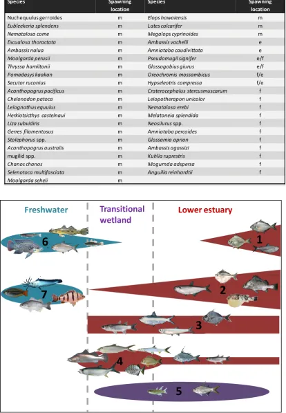
(5) Abstract A fundamental goal of ecology is to understand the mechanisms that regulate patterns of abundance, distribution, and richness of species’ across landscapes. Achieving this will ultimately help to inform better designed ecological surveys, improve predictive capabilities, and enhance efficacy of management and conservation measures. Although coastal systems provide valuable nurseries for commercially and recreationally important nekton species around the world, conceptual frameworks to facilitate understandings of their faunal patterns are scant. However, it is clear that models of coastal ecosystem function are becoming increasingly sophisticated, progressing away from fine-scale, single-scale focuses to incorporate more of the processes that underpin patterns. In this thesis I use Australian tropical estuaries as model systems to further develop ideas of coastal ecosystem functioning, by demonstrating how a hierarchy of processes interact across a broad spectrum of scales to shape local faunal outcomes in a coastal system. Some information on broader-scale processes shaping faunal pattern in Australian tropical estuaries already exists. Starting at the broadest scale, biogeographic factors regulate species pools, setting the limits on which species can potentially utilise estuaries in a region. At a finer scale, within a bioregion the supply of recruits into individual estuary systems is systematically modified by the location of coastal spawning grounds relative to estuary mouths, the existing population size of self-recruiting estuary resident species, and connectivity to permanent freshwater recruit sources. To determine how recruits from the three different sources (coastal marine, within the estuary, and from permanent freshwater reaches) typically distribute at finer scales, within an estuary system, catch data were compared across three different reaches spanning the entire length of the river-estuary axis (lower estuary, transitional wetlands, freshwater reaches). Patterns of distribution were diverse within the assemblage, varying in a speciesand life-history-specific manner, and emerging in 7 general ‘modes of dispersal’ along the estuary axis. Three of these modes describe varying levels of upstream dispersal by marinespawned species, while an additional group of marine-spawned species were unexpectedly biased towards upstream reaches. The other 3 modes consisted of uniformly distributed estuary-residents, and two groups of freshwater species with varying levels of dispersal into the upper reaches of the estuary. The interfacing of these diverse ‘modes of dispersal’ means that habitats embedded in different reaches of the estuary will be subjected to very different species pools.. iii.
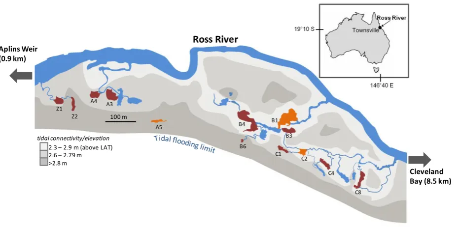
(6) Species pools in estuary reaches are not static however, but shift and morph seasonally in response to physico-chemical shifts and life-history cycles of estuary use. The nature and severity of seasonal shifts in faunal patterns were subsequently examined in the transitional zone of an estuary system, where the lower estuary and freshwater reaches interface. These transitional wetlands are the focus for extreme monsoon-driven physical shifts, and also subject to colonisation from all three recruitment sources. Fish were sampled on a monthly-bimonthly basis over 3 annual cycles, and trajectories of species’ abundance and modal size-class revealed a diversity of temporal cycles that could be split into 4 modes based on varying responses to physical shifts and the relevance of transitional wetlands in lifehistories of species. This included: (1) classic nursery cycles of post-larval recruitment, growth, and emigration, (2) nursery cycles periodically interrupted by freshwater flows/floods, (3) recruitment delayed until after freshwater floods – presumably as the species initial recruit to ephemeral wetlands associated with floods, and (4) year-round wetland residence and selfrecruitment. These diverse and complex patterns suggest that assemblages will vary markedly relative to time of year sampled, as well as occurrence, timing and extent of monsoonal floods. Following floods, transitional wetlands fragment to a series of tidally connected pools, providing a tractable system to examine finer-scale processes shaping spatial structure of assemblages in a coastal wetland system. Twenty pools were sampled through two annual cycles, to assess the relative influence of local (i.e. environmental constraints) vs. regional drivers (i.e. dispersal processes) on assemblage structure. Faunal patterns suggested that assemblages were primarily structured according to the level of hydrological connectivity with the estuary channel, and secondarily by local environmental conditions in pools. The assemblage can be broken up into two components based on responses to connectivity: an estuary generalist component constrained by connectivity to better connected pools closer to the estuary channel, and a wetland specialist component that seemingly ascended gradients of elevation to access pools further from the channel, perhaps reflecting a drive to access a unique nursery habitat. Additionally, among lower elevation pools, where frequent connections facilitated redistribution, there was some evidence of species sorting relative to preferred conditions (e.g. depth, substrate type). These results illustrate how different patches of seemingly similar habitat may perform different functions for the assemblage due to their position in the landscape. To evaluate the extent to which spatial patterns in the wetland system may have been influenced by interactions with other faunal groups (prey), during the pre-wet season month. iv.
(7) of October in two consecutive years, benthic invertebrate and zooplankton assemblages were sampled in a subset of 13 pools, concurrently with fish surveys. Linkages between distribution of fish and invertebrate prey suggested that the major assemblage split across the wetland may have partially been a response to prey sources as well as a function of pool accessibility. Moreover, prey distributions explained some patterns among the better connected pools, exhibiting patterns consistent with hypotheses of bottom-up control. These results highlight the importance of biological interactions as a key component of the spatial ecology processes structuring fish assemblages in coastal wetlands. It is clear that local faunal patterns in Australian tropical estuaries are ultimately a function of all of these levels of process working in concert - processes characteristic of broader scales inevitably constrain faunal pattern at finer scales. Thus, in its simplest form this hierarchy of processes can be perceived as a succession of spatio-temporally variable filters imposed at different scales that sequentially refine the assemblage as levels are descended. Placing traditional study sites (or focal patches) within the framework of a broader ecosystem, recognising the interaction of processes across multiple scales in time and space, will therefore allow us to better account for observed patterns, and enhance the efficacy of ecological studies in these systems. The general principle of this hierarchical framework is also applicable to other coastal and estuarine systems in other parts of the world, although the exact nature of processes and their relative influence on faunal outcome will vary from place to place.. v.
(8) Contents Statement of contribution from others............................................................................ i. Acknowledgements……………………………………………………………………………………………………………. ii. Abstract………………………………………………………………………………………………………………………….......... iii. List of figures………………………………………………………………………………………………………………………... vi. List of tables…………………………………………………………………………………………………………………………. viii. Chapter 1: General introduction – Understanding fish utilisation patterns in coastal and estuarine systems: history, progress, and future direction…………….. 1. 1.1 1.2 1.3 1.4. Trajectory of conceptual development…………………………………………………………………. Developing conceptual and operational frameworks……………………………………………. Dealing with scale multiplicity in complex systems.................................................. Australian tropical estuaries as a model system for developing frameworks……………………………………………………………………………………………………………. 1 5 7 10. Chapter 2: Varying patterns of fish distribution along Australian tropical estuaries...................................................................................................................................... 14. 2.1 Abstract…………………………………………………………………………………………………………………. 2.2 Introduction…………………………………………………………………………………………………………… 2.3 Methods………………………………………………………………………………………………………………… 2.3.1 Data collection……………………………………………………………………………………… 2.3.2 Data analysis………………………………………………………………………………………… 2.4 Results……………………………………………………………………………………………………………………. 2.4.1 Assemblage composition……………………………………………………………………… 2.4.2 Distribution patterns……………………………………………………………………………. 2.5 Discussion………………………………………………………………………………………………………………. 2.5.1 Modes of dispersal……………………………………………………………………………….. 2.5.2 Conclusion…………………………………………………………………………………………….. 14 14 16 17 22 23 23 26 29 29 33. Chapter 3: Temporal utilisation of estuarine wetlands with complex hydrological connectivity........................................................................................... 34. 3.1 Abstract…………………………………………………………………………………………………………………. 3.2 Introduction…………………………………………………………………………………………………………… 3.3 Methods………………………………………………………………………………………………………………… 3.3.1 Study site……………………………………………………………………………………………… 3.3.2 Fish sampling……………………………………………………………………………………….. 3.3.3 Data analysis………………………………………………………………………………………… 3.4 Results……………………………………………………………………………………………………………………. 3.4.1 Physical data………………………………………………………………………………………… 3.4.2 Patterns of fish utilisation…………………………………………………………………….. 3.5 Discussion………………………………………………………………………………………………………………. 3.5.1 Patterns of utilisation…………………………………………………………………………… 3.5.2 Linking pattern and process………………………………………………………………….. 34 35 37 37 37 38 39 39 40 45 45 47.
(9) Chapter 4: Seascape and metacommunity processes regulate fish assemblage structure in coastal wetlands…………………………………………………………………... 51. 4.1 Abstract…………………………………………………………………………………………………………………. 4.2 Introduction…………………………………………………………………………………………………………… 4.3 Methods………………………………………………………………………………………………………………… 4.3.1 Study site……………………………………………………………………………………………… 4.3.2 Fish sampling………………………………………………………………………………………… 4.3.3 Explanatory variables……………………………………………………………………………. 4.3.4 Data analysis………………………………………………………………………………………… 4.4 Results……………………………………………………………………………………………………………………. 4.4.1 Assemblage structure…………………………………………………………………………… 4.4.2 Individual species distribution………………………………………………………………. 4.5 Discussion………………………………………………………………………………………………………………. 4.5.1 Regional processes……………………………………………………………………………….. 4.5.2 Local processes…………………………………………………………………………………….. 4.5.3 Tidal pool vs. freshwater metacommunity dynamics……………………………. 4.5.4 Conclusions…………………………………………………………………………………………... 51 52 54 54 56 56 60 61 61 65 66 67 69 71 71. Chapter 5: Bottom-up control modifies patterns of fish connectivity and assemblage structure in coastal wetlands……………………………………………………….. 73. 5.1 Abstract…………………………………………………………………………………………………………………. 5.2 Introduction................................................................................................................ 5.3 Methods………………………………………………………………………………………………………………… 5.3.1 Study site……………………………………………………………………………………………… 5.3.2 Data collection……………………………………………………………………………………… 5.3.3 Data analysis………………………………………………………………………………………… 5.4 Results……………………………………………………………………………………………………………………. 5.5 Discussion……………………………………………………………………………………………………………….. 73 74 76 76 78 78 80 84. Chapter 6: General Discussion – Towards a holistic understanding of faunal pattern in tropical estuaries…………………………………………………………………………………. 88. 6.1 Hierarchy of processes…………………………………………………………………………………………… 6.1.1 Biogeographic distribution……………………………………………………………………. 6.1.2 Recruit supply………………………………………………………………………………………. 6.1.3 Patterns of dispersal along estuary profile……………………………………………. 6.1.4 Estuarine landscape structure………………………………………………………………. 6.2 Functioning of the hierarchy………………………………………………………………………………….. 6.2.1 Top-down cascade……………………………………………………………………………….. 6.2.2 Bottom-up mechanisms……………………………………………………………………….. 6.3 Periodic disturbances to hierarchical functioning…………………………………………………. 6.3.1 Intra-annual shifts in landscape use……………………………………………………… 6.3.2 Inter-annual regime shifts……………………………………………………………………. 6.4 Conclusion………………………………………………………………………………………………………………. 88 91 91 92 94 97 97 98 100 100 103 104. References…………………………………………………………………………………………………………………………….. 106. Appendices…………………………………………………………………………………………………………………………... 129. Appendix A: Pictures of Annandale Wetland………………………………………………………………... 129. Appendix B: Summary of total fish catch from Annandale Wetland…………………………….. 132. Appendix C: Consistency in assemblage structure through a semi-lunar cycle……………... 134.
(10) Appendix D: Site fidelity and movement patterns of individual barramundi (Lates calcarifer) through the study period…………………………………………………………………….. 139. Appendix E: List of publications arising from this thesis……………………………………………….. 144.
(11) List of figures Fig 1.1: Conceptual illustration of the 4 main types of movement influencing distribution across a coastal seascape, using the mangrove jack Lutjanus argentimaculatus as an example... 3. Fig 1.2: Conceptual model showing the predicted metacommunity dynamics given varying levels of dispersal and environmental heterogeneity/influence………………………………………………... 6. Fig 1.3: Diagram illustrating the nested organisational levels comprising a coastal seascape or estuary system………………………………………………………………………………………………………………………….. 7. Fig 1.4: Spatio-temporal domains of movement made by a typical marine-spawned coastal or estuarine fish through its life-cycle……………………………………………………………………………………………. 8. Fig 1.5: Diagram to illustrate the position of transitional wetlands within the sub/dry-tropical estuarine landscape………………………………………………………………………………………………………………….. 11. Fig 1.6: Thesis framework, showing the nested hierarchy of organisational scales that make up estuary landscape, and for which species-environment relationships are likely to influence assemblage structure………………………………………………………………………………………………………………... 13. Fig 2.1: Geographic location of transitional wetland sites…………………………………………………………. 17. Fig 2.2: Site map of Annandale Wetland showing the 20 pools…………………………………………………. 18. Fig 2.3: Site maps of transitional wetlands showing configurations of the sampled pools relative to permanent subtidal channels, and the approximate extent of tidal connections (based on satellite imaging)………………………………………………………………………………………………………. 20. Fig 2.4: Overlap of species recorded in each of the three reaches (lower estuary, transitional wetland, and freshwater)………………………………………………………………………………………………………….. 24. Fig 2.5: mCART of assemblage composition (based on Bray-Curtis dissimilarities) across the all lower estuary, transitional wetland, and freshwater sites…………………………………………………………. 25. Fig 2.6: Composite histogram of rank abundances (20=most abundant) of dominant species in each reach (±1 S.E. for lower estuary and freshwater rank abundances, which have been averaged over sites)………………………………………………………………………………………………………………….. 26. Fig 2.7: Conceptual model illustrating the range of dispersal modes contributing to differences in assemblages composition among reaches……………………………………………………………………………. 28. Fig 3.1: Freshwater flowing over Aplin’s Weir (solid line plot) from December 2009 to December 2011 (measured as mega-litres per day), and the resulting salinity changes in Annandale Wetland during the sampling periods of 2010 and 2011………………………………………….. 40. Fig 3.2: CPUE and modal size-class dynamics for taxa exhibiting patterns of classic nursery utilisation (CNU)………………………………………………………………………………………………………………………... 42. Fig 3.3: CPUE and modal size-class dynamics for taxa exhibiting patterns of delayed recruitment (DR)……………………………………………………………………………………………………………………….. 43. Fig 3.4: CPUE and modal size-class dynamics for taxa exhibiting patterns of interrupted persistence (IP)………………………………………………………………………………………………………………………... 44. vi.
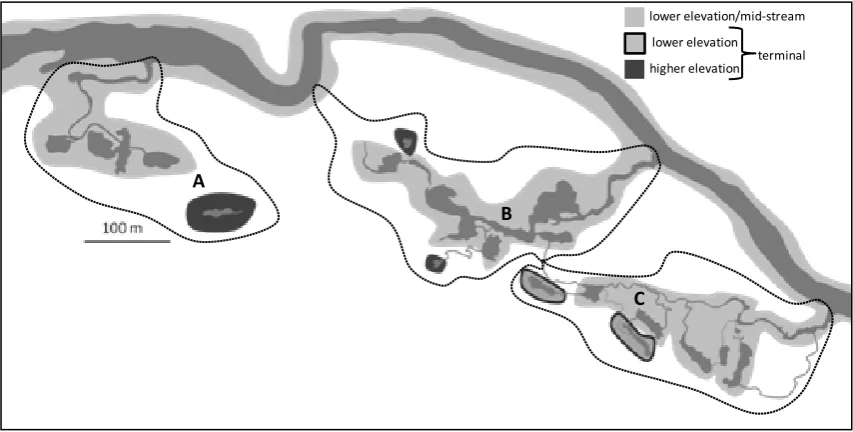
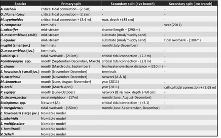
(12) Fig 3.5: CPUE and modal size-class dynamics for taxa exhibiting patterns of facultative wetland residence (FWR)……………………………………………………………………………………………………………………….. 45. Fig 4.1: Anndandale Wetland containing the 20 wetland pools adjacent to the Ross River, Australia…………………………………………………………………………………………………………………………………... 55. Fig 4.2: mCART of log(CPUE+1) based on pool codes, month, and year, explaining 21% of the variation in assemblage structure…………………………………………………………………………………………….. 61. Fig 4.3: mCART of log(CPUE+1) based on (a) explanatory variables and (b) all explanatory variables except ‘critical tidal connection’………………………………………………………………………………... 64. Fig 4.4: Map of the wetland illustrating heterogeneity in fish assemblages, derived from pool groupings in Figs 4.3 a & b…………………………………………………………………………………………………………. 65. Fig 4.5: Conceptual models illustrating how assemblages are structured in (a) freshwater mainland-island type metacommunities, based on trends in the literature (Snodgrass et al. 1996, Taylor 1997, Magnuson et al. 1998) and (b) in tidal systems of similar topological configuration based on results of the present study…………………………………………………………………. 70. Fig 5.1: Annandale Wetland containing the 22 wetland pools adjacent to the Ross River, Australia……………………………………………………………………………………………………………………………………. 76. Fig 5.2: Univariate classification and regression trees displaying the distribution of zooplankton (calanoid copepods) in (a) 2010, and (b) 2011, based on log(CPUE+1) data………….. 81. Fig 5.3: Non-metric multidimensional scaling (nMDS) ordination, using Bray-Curtis dissimilarities on log(CPUE+1) benthic invertebrate assemblage data in 2010 and 2011…………... 82. Fig 5.4: nMDS ordination, using Bray-Curtis dissimilarities on log(CPUE+1) fish assemblage data in 2010 and 2011………………………………………………………………………………………………………………. 82. Fig 5.5: Likely food-webs underpinning patterns of community assembly in (a) lower elevation pools, and (b) higher elevation pools……………………………………………………………………………………….. 85. Fig 6.1: Figurative representation of patterns and processes constraining assemblage composition at a range of scales, based on outcomes of the data chapters……………………………... 89. Fig 6.2: a) Hierarchy of organisational scales at which key processes operate, and b) a hierarchical framework model, illustrating linkages among pattern and process over this multiplicity of organisational scales…………………………………………………………………………………………... 90. Fig 6.3: A conceptual life-history schedule of E. hawaiensis illustrating ontogenetic migrations and home-range extents…………………………………………………………………………………………………………... 99. Fig 6.4: Common components of the tropical estuary habitat mosaic………………………………………. 102. vii.
(13) List of tables Table 2.1: Sources of data used to estimate assemblages of species in lower estuarine reaches and permanent freshwater streams of the bioregion……………………………………………………………….. 22. Table 2.2: Spawning locations of various species, assisting the identification of the different dispersal modes……………………………………………………………………………………………………………………….. 28. Table 3.1: Approximate body lengths at important life-history landmarks for taxa recruiting to the wetland at small size classes (<40 mm FL), to determine how wetland utilisation patterns relate to life-histories………………………………………………………………………………………………………………... 41. Table 3.2: Early life history parameters of species only caught at advances sizes……………………... 43. Table 4.1: Description of the explanatory variables derived to explain spatial structure of the fish assemblage………………………………………………………………………………………………………………………... 57. Table 4.2: Results from univariate CART’s of log(CPUE+1) of individual species………………………... 66. Table 5.1: Environmental variables used in the BIO-ENV and CART procedures, to test for correlations with benthic invertebrate, fish, and zooplankton data………………………………………….. 77. Table 5.2: Trophic function of abundant fish taxa in Annandale Wetland…………………………………. 83. Table 5.3: Results of BIO-ENV analyses……………………………………………………………………………………. 83. viii.
(14) Chapter 1 – General Introduction. Understanding fish utilisation patterns in coastal and estuarine systems: history, progress, and future direction Estuaries and adjacent inshore coastal wetlands have long been regarded as nurseries for a diversity of nekton, many of high commercial and recreational value. However, detailed understanding of the spatial ecology of fish in these systems has been slow to evolve. By extension, our knowledge of the functional utilisation of coastal and estuarine ecosystems is incomplete, and substantial levels of faunal complexity remain unresolved. A combination of factors has contributed to this slow progress. Most evidently, the characteristic high turbidities of many estuaries has restricted the use of direct visual observations, which have been the mainstay of studies of pattern and process in freshwater streams (Hankin & Reeves 1988) and coral reef systems (Brock 1982). The resulting reliance on a mix of sampling gears, each suitable for sampling different estuarine environments, has limited direct comparison of catches within and among estuarine systems (Rozas & Minello 1997). Meanwhile, a bias of studies and theoretical development toward certain geographical and climatic zones (Rozas 1995) has limited assessment of generalities and global relevance of findings (Blaber 2002, Faunce & Serafy 2006). However, arguably the most profound impediment to our understanding has been the slow development of conceptual frameworks of ecosystem function in which to develop theories and direct further study. 1.1 Trajectory of conceptual development Early studies of fish fauna in estuaries were largely descriptive, neglecting ecological drivers of pattern and effectively perceiving estuaries as homogenous entities (McErlean et al. 1973, Hardisty & Huggins 1975, Blaber 1980). Several fish ecologists then began to investigate responses to gradients of salinity and turbidity that characterise the physical environment of estuaries (Blaber & Blaber 1980, Whitfield et al. 1981, Cyrus & Blaber 1987b, 1992, Barletta et al. 2005, Barletta et al. 2008). These studies, largely based on correlations between species occurrences and physical readings, yielded some valuable information on varying physiological tolerances, but were ultimately predicated on over-simplistic concepts. Fish distributions are likely to be complicated by a range of factors at multiple spatial and temporal scales, beyond conditions at the immediate time and vicinity of capture (Pittman & McAlpine 2003). 1.
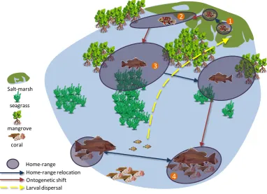
(15) Moreover, many species adapted to exploit estuaries are likely to possess broad physiological tolerances, enabling persistence in a habitat in spite of broadly variable physical conditions (Elliott et al. 2007). As the spatial resolution of sampling increased, species affinities for different constituent habitats of the estuary and coastal system emerged, including mangrove forests, salt-marshes, open channel, nearshore coastal waters, seagrass meadows (Blaber et al. 1989, Rozas & Minello 1998, Guidetti 2000, Bloomfield & Gillanders 2005). Subsequent efforts to explain faunal pattern (e.g. abundance, diversity, species richness) within these habitat types were primarily based on correlations with micro-habitat variables measured within the scale of the focal patch (i.e. the studied unit of habitat), such as seagrass blade density and stem length (Bell & Westoby 1986, Attrill et al. 2000), mangrove root complexity (Rönnbäck et al. 1999), epiphyte biomass (Gratwicke & Speight 2005), sediment characteristics, and local geomorphology (Allen et al. 2007). While it is evident that these fine-scale variables exert some influence over fish distribution (Heck & Orth 1980, Orth et al. 1984, Bell & Westoby 1986), much faunal variability often remains unexplained (Harris & Heathwaite 2012), suggesting overlooked processes may significantly influence local assemblage patterns. 1.1.1 Incorporating a spatial element When we consider the movements that coastal fishes make through daily routines, and through the trajectory of their lives, it is clear that sampling sites that have typically been the focus of ecological studies constitute small elements of a much bigger picture. Most coastal nekton species have a tri-phasic life-cycle (Fig 1.1), characterised by the ingress of eggs and larvae from offshore spawning grounds into inshore coastal waters and estuaries (Elliott et al. 2007, Cowen & Sponaugle 2009, Sheaves et al. 2013). This is followed by a period of growth, where routine shelter and foraging movements maintain a home-range in a certain area (McGrath & Austin 2009, Nagelkerken et al. 2013), the extent and shape of which is shaped by spatial patterns in benthic habitat structure (Pittman & McAlpine 2003, Hitt et al. 2011). During this period species make ‘ontogenetic migrations’, shifting and/or expanding their home range to incorporate different habitat types as their resource requirements change with growth and development (Cocheret de la Moriniere et al. 2002, Caddy 2008), and finally migrations from adult habitats back to spawning grounds close the cycle (Sheaves et al. 1999). This range of movements across the marine landscape means that local faunal patterns are partially driven by landscape patterns and processes operating at broader scales than previously studied. Based on this premise, a patch of high intrinsic habitat quality may be 2.
(16) depauperate of nekton, while a seemingly low quality site may teem with life as a consequence of surrounding landscape structure (Skilleter et al. 2005). To more reliably explain faunal distributions we therefore need to perceive focal sites as being embedded in a broader landscape. This perspective has long been embraced in the study of terrestrial systems, and forms the basis for the field of spatial ecology, which incorporates spatiallyexplicit information of landscape structure (i.e. the spatial configuration and composition of habitats across an expanse of interest) into ecological studies (Simberloff & Abele 1976, Forman & Godron 1986).. 2. 1. 3 Salt-marsh seagrass. mangrove coral Home-range Home-range relocation Ontogenetic shift Larval dispersal. 4. Figure 1.1: Conceptual illustration of the 4 main types of movement influencing distribution across a coastal seascape, using the mangrove jack Lutjanus argentimaculatus as an example. Numbers in orange illustrate the stage in a sequence of ontogenetic progressions.. Considering the influence of landscape structure on patterns and processes first means detecting and defining it. There are two main ways of conceptualising and analysing landscape structure, which have been developed in terrestrial systems, and subsequently applied to marine systems: the binary patch-matrix model, and the landscape mosaic model. These two models are each appropriate for tackling different ecological questions at different conceptual scales, although sometimes offer complementary ways of modelling animalenvironment relationships (Haila 2002).. 3.
(17) Binary landscapes The most basic form of modelling and analysing spatial heterogeneity in the environment is to view the landscape as a binary system of usable habitat patches embedded in a less hospitable background habitat (called a matrix) (Forman & Godron 1981, Davies et al. 2001, Fahrig 2002). This perspective derives from the field of island biogeography, which recognises how the size of islands and their distance from a mainland stock of colonists affects their species richness and biodiversity (Simberloff & Abele 1976), by influencing colonisation and extinction rates (MacArthur & Wilson 1967). Most habitats, analogous to islands, exist as a fragmented complex of patches embedded in a hostile background matrix (e.g. forest patches in an agricultural setting). These patches harbour spatially separated populations and communities, connected by movements of individuals over a range of time scales (Hanski 1991), emphasising the importance of spatial context of patches as well as the internal characteristics (Forys & Humphrey 1999). In highly fragmented habitats the viability of a regional population is often dependant on dispersal between disparate sub-populations occupying patches (Hanski 1999). Ecologists have examined how spatial features of these ‘metapopulations’, including the size, number, and spatial arrangement of patches (e.g. relative patch isolation), influence the dispersal of individuals among sub-populations (Gustafson & Gardner 1996, Hein et al. 2004, Fahrig 2007). ‘Landscape ecology’ approaches have since developed these ideas, to link faunal patterns in terrestrial systems to a more realistic representation of spatial heterogeneity in the landscape. For instance, landscape ecology models have considered how detailed geometric features such as patch shape, isolation, inter-patch distance, clumping of patches, and edge characteristics (Turner 1989, Moilanen & Hanski 1998, McGarigal 2002), shape movement patterns of individuals across the landscape, and result in spatial variations in species abundance and community structure (Diffendorfer et al. 1995, Bender et al. 2003). Many marine habitats can be viewed as submerged binary landscapes akin to those on land. However, only relatively recently have coastal ecologists started to break beyond a finescale, single-scale focus to explicitly incorporate the role of landscape structure into studies of faunal complexity. Such studies have largely been focussed around seagrass meadows, which naturally exist as a binary system of vegetational units embedded in a bare substrate matrix, lending themselves to spatially-explicit interrogation (Robbins & Bell 1994, Turner et al. 1999, Hovel et al. 2002, Bostrom et al. 2006, Jackson et al. 2006b). However, a range of 4.
(18) complications associated with working in open systems have meant that the influence of landscape-level features remain equivocal. A prominent issue in coastal spatial ecology is defining landscape structure at scales relevant to the patterns of species utilisation (Pittman & McAlpine 2003). Without information on movement patterns of individuals, or distribution data across a nested multiplicity of scales (Holland et al. 2004), study areas cannot be reliably scaled to match species’ windows of spatial perception (Pittman & McAlpine 2003, Connolly & Hindell 2006, Grober-Dunsmore et al. 2009), which inevitably com promises meaningful ecological inference (Pittman & McAlpine 2003). Further obscuring ecological inference, factors related to sampling artefacts, the dynamic occurrence of fish in patches (Jackson et al. 2006b), and behaviours such as schooling, generate considerable noise in analyses (Connolly & Hindell 2006). Parallel shifts in perspective, progressing beyond a fine-scale, single-scale focus, have also characterised recent conceptual developments in freshwater ecology. Community structure and dynamics in patches such as lakes, ponds, and stream pools, were traditionally examined in the context of local abiotic and biotic conditions (Leibold et al. 2004). Current models now incorporate movements among these patches by conceiving local communities as part of a broader ‘meta-community’, where patches are connected by a common regional species pool (Brown & Swan 2010). By simultaneously considering the influence of local processes (i.e. environmental constraints in patches) and regional processes (i.e. organism connectivity among patches), these studies offer new insights into faunal structure of wetland systems. In contrast to many coastal wetlands, fragmented freshwater systems consist of highly discrete patches that are inter-connected through easily defined pathways (e.g. channels), and embedded within an uninhabitable terrestrial matrix. Since fish are restricted to patches and the constrained pathways connecting them, there is high explanatory power in partitioning the relative influence of local and regional processes, providing a fertile ground for developing understandings in spatial ecology (De Meester et al. 2005). Several paradigms have emerged from metacommunity ecology, predicting how communities will be structured by varying levels of ‘local’ and ‘regional’ influence under different scenarios (Leibold et al. 2004, Winegardner et al. 2012) (Fig 1.2). For instance, the ‘species-sorting’ paradigm predicts that if hydrological/structural connectivity is sufficient to allow dispersal across a heterogeneous landscape, species will distribute according to niche processes. However, if dispersal rates are particularly high, regional effects may swamp local effects by enabling persistence of species in sub-optimal patches (i.e. a ‘spill-over’ effect), as predicted by the ‘mass-effect’ paradigm (Logue et al. 2011). If fragmented coastal wetlands similarly behave as a binary patch-matrix 5.
(19) system, then principles emerging from metacommunity ecology are equally applicable to coastal habitats, and can be useful in resolving the drivers of pattern.. Dispersal Environmental constraints. Neutral model: Mass effect: Homogenous Spill-over into distribution potentially suboptimal patches. Species sorting: Assortment of species among patches relative to resources/niches. Patch dynamics: Low dispersal means assemblage reflects local processes occuring within patches. Figure 1.2: Conceptual model showing the predicted metacommunity dynamics given varying levels of dispersal and environmental heterogeneity/influence.. Landscape mosaics In many scenarios limiting spatial ecology studies to a single habitat type only tells part of the story (Law & Dickman 1998, Pittman & McAlpine 2003), since organisms rely on a multitude of habitat types through routine daily functions (Hansson et al. 1995, Nagelkerken et al. 2013), and as they transition through ontogeny (Cocheret de la Moriniere et al. 2002, Caddy 2008, Snover 2008). Therefore, the composition (i.e. the abundance and richness of different habitat types) and configuration of disparate habitats within a landscape has strong implications for how a system operates for the faunal assemblage, by promoting or inhibiting functional connectivity (Wiens et al. 1993, Guerry & Hunter 2002, Grober-Dunsmore et al. 2009). To incorporate this ecological complexity into models of faunal pattern, landscape ecologists began viewing the landscape as a mosaic of functionally connected habitat components. In this model patches constitute units of multiple potentially interacting habitat types that provide complementary resources for animal assemblages (Dunning et al. 1992, Taylor et al. 1993, Wiens 1995). Recently, the mosaic approach has been applied to marine landscapes or ‘seascapes’ (Grober-Dunsmore et al. 2009, Bostrom et al. 2011), defined here as a heterogenous marine or intertidal environment, consisting of patches of multiple habitat types (e.g. mangrove, seagrass, sandy substrate, rocky reef). Like terrestrial animals, nekton perceive their environment as a mosaic of complementary resources, moving between different habitat types through routine tidal and diel movements (Kendall et al. 2003, Verweij & Nagelkerken 2007, Hitt et al. 2011), and also through longer-term ontogenetic migrations (Nagelkerken et al. 2001, Cocheret de la Moriniere et al. 2002, Unsworth et al. 2008) (Fig 1.1). 6.
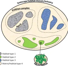
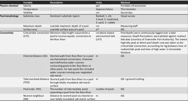
(20) The influence of landscape mosaic patterns on faunal patterns in coastal systems is demonstrated by greater species richness and abundances in both mangroves (Pittman et al. 2004), and salt-marshes (Irlandi & Crawford 1997), adjacent to seagrass beds and vice-versa (Jelbart et al. 2007), than at sites where these habitats are far apart. Such ‘seascape connectivity’ often explains more site-to-site variability in assemblage structure than local habitat attributes (Skilleter et al. 2005, Olds et al. 2012), and is therefore a crucial consideration when explaining faunal pattern in coastal and estuarine systems. 1.2 Developing conceptual and operational frameworks in coastal systems It is clear that models of coastal ecosystem functioning are becoming increasingly sophisticated. Ecological research in these systems was originally predicated on intuitive human-based perceptions of habitat, often focussing at scales markedly finer than routine daily movements. With developing knowledge and technical capabilities, these ideas are giving way to more holistic multi-scale approaches that more accurately reflect the manner in which fish use the landscape (Pittman et al. 2007a, Whaley et al. 2007, Green et al. 2012, Olds et al. 2012), recognising that local faunal patterns are the product of patterns and processes operating over a range of scales. Current. seascape. approaches factor in three main spatial and conceptual scales of focus: the mosaic of habitat types within a coastal system, the landscape attributes of a single habitat type (i.e. a habitat complex), and the micro-habitat attributes of a patch (Fig 1.3). This framework encompasses and. Figure 1.3: Diagram illustrating the nested organisational levels comprising a coastal seascape or estuary system. For simplicity, the patches of habitat have been presented as part of discrete habitat complexes (demarcated by dotted lines). However, patches of habitat types can also be interspersed among each other, such that habitat complexes overlap. In some models the matrix may be considered as an additional potentially important habitat type, although many models simply consider structural connectivities between habitat units embedded within the matrix.. 7. accounts. for. processes. associated. with. foraging. movements,. tidal. excursions,. home-range shifts, and some ontogenetic shifts (Fig 1.4). It is apparent however, that the scope of this framework is still.
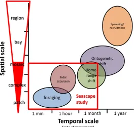
(21) limited, as movement patterns of many coastal fishes extend beyond the boundaries of this spatio-temporal domain. We therefore need to further expand the realm of scales recognised in conceptual and operational frameworks, both in time and space. Spatial variation in recruitment from spawning grounds, and perhaps effects of broader-scale ontogenetic movements (e.g. cross-shelf migrations), will also engender substantial variability in faunal pattern. Meanwhile, gradients in physico-chemical conditions (i.e. salinity, temperature, and turbidity) of the water mass surrounding habitat mosaics may also constrain the distribution of species’ across coastal wetlands and estuaries (Rakocinski & Fleeger 1992, Pittman et al. 2007a). While recruit supply and physico-chemical gradients are not necessarily overlooked, they are difficult to incorporate into seascape models as they typically do not relate to spatially-explicit features of the landscape, and have an apparent nebulous influence on faunal pattern. Due to the high labour demands of repeated sampling, region. seascape. Spatial scale. Spawning/ recruitment. studies. also. rarely. incorporate a temporal dimension (Bostrom et al. 2011). Patterns of. bay. recruitment in coastal systems are mosaic Tidal excursion. complex. Ontogenetic shift Homerange shift. highly seasonal however (YåñezArancibia et al. 1988, Barletta et al. 2008, Green et al. 2009), and as species. Seascape study. foraging. patch 1 min. 1 hour. pools. and. conditions. change through the year, the. 1 month. 1 year. influence of landscape features and environmental heterogeneity. Temporal scale (rate of movement). Figure 1.4: Spatio-temporal domains of movement made by a typical marine-spawned coastal or estuarine fish through its life-cycle. The red box represents the spatio-temporal domain accounted for in current seascape frameworks, and the filled section of the red arrow represents the organisational levels at which movements/processes are currently considered.. on assemblage structure are also likely to vary (Hovel & Fonseca 2005, Johnson & Heck 2006). Another. notable. limitation. of. seascape studies is the unilateral focus on a single faunal group (i.e. nekton) (GroberDunsmore et al. 2009, Bostrom et al. 2011), despite the likelihood that biological interactions with other faunal groups (e.g. benthic infauna, zooplankton, crabs) will play a substantial role in shaping distribution of species (Hovel & Regan 2008). Predator-prey interactions however,. 8.
(22) are notoriously difficult to quantify in open coastal waters, as feeding grounds may only represent a small component of daily home-ranges (Sheaves 2009). 1.3 Dealing with scale multiplicity in complex systems Faunal patterns can only be fully understood by an explicit consideration of phenomena at multiple scales, since different processes prevail and generate characteristic variability in animal assemblages across a range of spatial-temporal domains (Allen & Starr 1982, Levin 1992, MacKey & Lindenmayer 2001). The integration of ecological phenomena across a broad range of scales can be a difficult concept to grasp and implement however, and as we increasingly acknowledge the complexity of coastal ecosystems, we will need to develop models in which to frame and simplify multi-scale functioning. Hierarchy theory provides a conceptual framework to deal with scale multiplicity in complex systems, and to facilitate a holistic approach to understanding biological patterns. Hierarchy theory recognises that complex systems can be broken down into discrete functional levels based on organisational scales and rates of process characteristic of these scales (Allen & Starr 1982, Urban et al. 1987, Wu & David 2002). Landscapes can be perceived to exist as multiple nested scales of discrete functional components that correspond to levels in the hierarchy (Kotliar & Wiens 1990). For example, forested landscapes can be broken down into a nested hierarchy of gaps (0.01-0.1 ha), forest stands (1s-10s ha), watersheds (100s1000s ha), and physiographic provinces (10000 ha) (Urban et al. 1987). Meanwhile, in marine systems seagrass has similarly been described and analysed as a hierarchy of nested spatial structures, ranging from shoots at the finest scale (mm’s), to clumps (cm’s – m’s), which aggregate to form patches (1-100 m), and at a greater scale meadows (km’s), surrounded by a mosaic of disparate habitat types, such as mangroves and coral (Robbins & Bell 1994, Pittman & McAlpine 2003). In the hierarchy, higher levels typically correspond with broader spatial scales, where processes characteristically operate at slower rates. Meanwhile lower levels correspond with smaller spatial extents and finer scales, where processes characteristically operate relatively rapidly (O'Neill 1986). Due to the disparity in process rate between hierarchical levels, relationships between adjacent levels are asymmetric, with landscape patterns and ecological processes at higher levels appearing as constants and exerting constraints on the biological dynamics of lower levels (Urban et al. 1987). For instance, using the example of forested landscapes, broad-scale physiographic features such as mountain ranges may influence the local climate and dispersal of propagules between watersheds, in turn limiting the plant species capable of colonising and settling in a watershed. Conversely, 9.
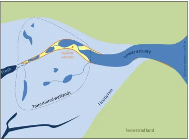
(23) lower level dynamics can often provide a mechanistic understanding towards biological dynamics at the next higher level (Urban et al. 1987), e.g. photosynthetic activity at the level of individual trees will manifest in biomass at the level of a stand. In aquatic systems, hierarchy theory has been interpreted and appropriated in different ways to inform conceptual and analytical models of faunal pattern. For instance, to examine how structural landscape patterns influence faunal pattern of nekton in inshore coastal wetlands, Pittman & McAlipne (2003) integrated a three-level hierarchy proposed by Allen & Starr (Allen & Starr 1982). In this model the intermediate (or focal scale) is anchored in time and space by the scales relevant to the phenomena of interest. For example, to examine distributions through daily routine functions, the focal level would be anchored at the scale of the home-range, which for many species may correlate with a mosaic of habitat patches in the seascape. At the lower level, finer-scale features of the landscape, such as seagrass leaf length, may influence distributions during portions of the home-rage and provide a mechanistic explanation for faunal patterns at the focal level. Meanwhile, at the higher level, broad-scale environmental features surrounding the home-range, such as gradients in wave action and salinity may lead to different faunal patterns over greater spatial extents or over time, but can be perceived as constants at the spatio-temporal domain of the study. Poff (1997) on the other hand advocated a top-down approach to modelling fish distributions in streams, conceptualising the riverine landscape as a nested sequence of filters, whereby environmental constraints acting at different organisational scales (from watersheds to valleys to stream reach to microhabitats) interact with species’ functional traits to shape and progressively refine the assemblage as scales are descended. The mechanistic understanding that underpins this approach allows for greater generalisation in applying a predictive framework across different systems and regions (Levin 1992). 1.4 Australian tropical estuaries as a model system for developing frameworks Tropical Australian estuaries provide an ideal model system in which to partition the influence of different levels of process spanning a broad spectrum of scales. They also present an opportunity to examine types of processes not typically considered in coastal seascape studies. Each estuary system naturally exists as a relatively discrete, semi-enclosed unit, as opposed to the diffuse, open nature of coastal seascape systems. Since recruits to estuaries primarily originate from external sources offshore (Sheaves et al. 2013), with little subsequent redistribution among estuaries, variable recruit supply can be indirectly assessed through estuary-to-estuary differences in assemblage composition (Sheaves et al. in review). Further, 10.
Figure
+7

Outline
Related documents
