Estimating the prevalence of the ‘toxic trio’ of family issues for each local area in England: Predictions based on spatial microsimulation methods: Vulnerability technical report 2: July 2019

(1)

Predictions based on spatial microsimulation methods

Vulnerability technical report 2

JULY 2019

(2)

1 Author: Tom Clarke, Senior Quantitative Analyst, Children’s Commissioner’s Office

(3)

2

Introduction and aims

This paper sets out in detail the methodology used by the Children’s Commissioner’s Office (CCO) to produce its estimated local area prevalence rates of children in households experiencing combinations of the ‘toxic trio’. In keeping with previous research, the ‘toxic trio’ refers to children in a household where a parent has experienced combinations of:

> Domestic violence/abuse (DV&A) > Substance misuse problems > Mental health problems

In 2018 the CCO produced the first ever national-level prevalence estimates of these issues and

combinations thereof (Chowdry 2018). This used data from the 2014 Adult Psychiatric Morbidity survey (APMS source: NHS Digital), a nationally representative survey of private households in England. The APMS has previously been used to provide the official national estimates of the prevalence of adult mental health and substance misuse problems.

[image:4.595.35.562.352.493.2]

This national level analysis in Chowdry (2018) presented prevalence levels based on both broad and narrow measures of each of the constituent parts of the toxic trio. These broad and narrow measures were:

Table 1: Broad and narrow measures of the toxic trio factors

Toxic trio

indicator Broad measure Narrow measure

DV&A Adult has ever experienced DV&A Adult has experienced DV&A within last year

Substance

misuse Adult reports any substance misuse Adult reports having a alcohol or drug dependency Mental

ill-health Adult has moderate or higher symptoms of mental or psychiatric disorders Adult has severe symptoms of mental or psychiatric disorders

For further information on the exact definition of these measures, see Chowdry (2018).

The modelling presented in this paper aims to extend this national level analysis by estimating the prevalence of these issues within each English upper tier local authority (LA) and parliamentary constituency (PC).

Challenges and limitations

It is important to state from the outset that there is no available, consistent data on the local prevalence of these issues based on actual surveys or other data collections. The modelling presented in this paper is a way of generating evidence-based predictions for each local area in the absence of such data. These predictions are based on statistical models estimated using the APMS and as a result should be treated as experimental in nature. They are intended as a first attempt based on data available for further refinement and validation.

(5)

4

Instead, the methodology we use here generates estimates by combining statistical modelling carried out on the APMS with other data on the known characteristics of each local area. This is commonly done for other survey based indicators where local area estimates are difficult to obtain - see for example small area income estimates (ONS, 2016). However, this should be borne in mind when interpreting the results and further information such as local surveys or administrative data would be useful to validate these

predictions.

Summary of spatial microsimulation approach used

One particular challenge with the APMS data is that geographical information about the respondents was not provided in it. This is unsurprising and necessary for privacy reasons given that the survey asks

respondents a variety of extremely sensitive questions. However, this lack of geographic identifier rules out hierarchical modelling approaches to this estimation as information on the local area cannot be linked to a respondent in the survey.

Instead this analysis uses spatial microsimulation to estimate these rates, an approach used extensively in human geography (see, for example Tominitz et al 2008). At a high level, this works through reweighting the individual level responses to a survey that is representative of a larger geography (in this case England) so that the profile of its respondents is representative of the population in a smaller geographical unit (in this case an LA or a PC).

To do this involves three main steps:

1. Determine key variables (constraint variables) in the survey dataset related to the ‘toxic trio’ outcomes that are also available at upper tier LA/PC level from sources such as the Annual Population Survey, 2011 Census, House of Commons Library, official statistics or other published data. The choice of the final set of constraint variables is determined both by their predictive power within the APMS and by the availability of an equivalent local-level variable.

2. Reweight the APMS sample to be representative of each LA/PC based on these constraint variables. In other words we calculate 1511_{sets of sample weights, each one designed to make the APMS resemble}

the profile of a particular LA; along with a further 533 sets of weights, each one designed to make the APMS resemble the profile of a particular English PC.

3. For each LA or constituency, we replicate the analysis carried out in Chowdry (2018), but using our new sample weights as described above, rather than the national population sample weights provided in the APMS.

Another relevant analysis that is more similar in context, if not in methodology, is the important work by Pryce et al. (2017) who use statistical modelling on the APMS to produce prevalence estimates of alcohol dependence for each LA in England, on behalf of Public Health England. In particular, they run ordered probit models where the dependent variable is an individual respondent’s severity of alcohol dependence, and the independent variables are their age, gender, quintile of deprivation, and linked region-level

information on rates of hospitalisation for alcohol-related issues.

The approach here is similar in nature but has an advantage in that it uses a wider range of information in the APMS, and is implemented in a more flexible manner that allows additional interactions between variables. However, both approaches have limitations (see below). We do not attempt to re-estimate these alcohol dependence estimates but instead incorporate them into our model as a constraint variable. This allows us to avoid duplicating these estimates while also building on this work.

(6)

5

Detailed methodology

Variable selection

The first step of this analysis was an iterative process of scanning variables available in the APMS survey that had equivalents reported at an LA/PC level to produce a list of candidate constraint variables.

> We searched for a range of available candidate variables by LA which were measures of demographic, socio-economic and household characteristics. However, we also made use of the aforementioned LA-level estimates of alcohol dependence prevalence, as well as estimates of the prevalence of common mental health disorders by LA (see Table 2 for data sources).

> Since PCs are an electoral geography rather than an administrative one, less information is available for these areas. This means that the modelling in the APMS necessarily uses fewer constraint variables in order to produce predictions for PCs. The characteristics we employed are largely sourced from the 2011 Census and relate to household and demographic characteristics, though more recent

information on benefit claimants was also available.

> Very few factors were available specific to households with children at any local area. However, some local authority estimates of alcohol and drug misuse prevalence have previously been published by Public Health England (Source: PHE 2018). To avoid duplication we do not re-estimate these at a local authority level but incorporate them into our modelling (where they are based on APMS data) or use them for validation purposes.

(7)

[image:7.792.48.605.64.533.2]

6

(8)

7

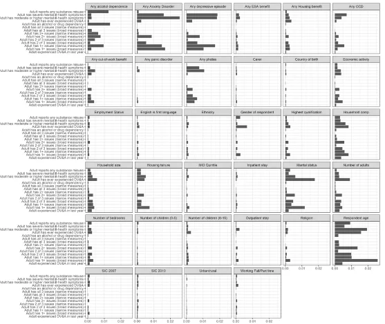
We limited our eventual set of constraint variables to those where both of the following conditions are satisfied:

1. The variable importance scores higher than 0.003 in any model in the plot above

2. A local area equivalent of the survey variable can be found at the required geographic level, with the same categorical/coding structure

The inevitable consequence of the second condition above is that while the models for LA predictions and PC predictions are based on the same approach, they involve different sets of constraint variables. In particular, the model for generating PC predictions is a restricted model using fewer constraint variables.

[image:8.612.42.569.237.554.2]

Based on data available at a LA level, we use the following constraint variables to predict LA prevalence rates:

Table 2: Final constraint variables included in LA weighting and sources for target proportions

Survey variable Source for LA level equivalent

Respondent age ONS 2017 LA population estimates

Any alcohol dependence PHE LA prevalence estimates 2016/17

Any out-of-work benefit DWP benefit claimant counts by LA at March 2018

Any depressive episode PHE common mental health disorders prevalence estimates 2016/17

Economic activity Annual Population survey 2016/17

Highest qualification Annual Population survey 2016/17

Any Generalised Anxiety Disorder PHE common mental health disorders prevalence estimates 2016/17

Household composition Census 2011

Household size Annual Population survey 2016/17

Any Housing benefit DWP benefit claimant counts by LA at March 2018

Marital status of respondent Census 2011

Any OCD PHE common mental health disorders prevalence estimates 2016/17

Any phobia PHE common mental health disorders prevalence estimates 2016/17

Gender of respondent ONS 2017 LA population estimates

Housing tenure Census 2011

As stated above, a smaller set of factors had to be used in the modelling for the PC model:

Table 3: Final constraint variables included in PC weighting and sources for target proportions

Survey variable Source for PC level equivalent

Respondent age ONS 2017 LA population estimates

Economic activity Census 2011

Highest qualification Census 2011

[image:8.612.33.578.610.724.2]

(9)

8

Household size Census 2011

Any Housing benefit DWP benefit claimant counts by constituency at March 2018

Marital status of respondent Census 2011

Gender of respondent ONS 2017 LA population estimates

Housing tenure Census 2011

Any out-of-work benefit DWP benefit claimant counts by constituency at March 2018

Note that many of these measures date back to 2011, and therefore may not be good indications of the

current profile and characteristics of PCs. This remains a caveat and limitation when attempting to produce

[image:9.612.36.575.39.171.2]

PC-level estimates.

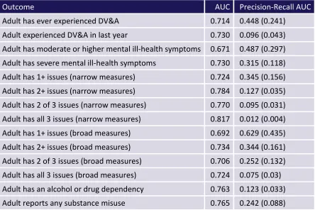
Table 4 and Table 5 demonstrate the predictive power based on AUC and precision recall AUC measures for each outcome measure, for the LA and PC models respectively. The AUC provides an indicator of classification performance based on true positive and true negative rates at varying classification thresholds: a value of 0.5 indicates no predictive power, while a value of 1 indicates a perfect classifier. This is useful except where there is a large imbalance between positive and negative classes as the true negative rate will always be high where there are a large number of negative cases. AUC values are appropriate when the observations are balanced between each class, whereas precision-recall AUC values are appropriate for imbalanced classes.

This is particularly the case when considering the ‘All 3’ outcome – i.e. the presence of domestic violence, substance misuse and mental health issues. The overall prevalence of this outcome is much lower. Precision-recall AUC therefore provides a better metric as it focuses only on the accuracy of prediction for the positive cases. Again a perfect classifier would score 1 on a precision-recall AUC measure, however models should be interpreted based on how they perform compared to a random classifier (provided in brackets in the table below).

These tables suggest that for both sets of estimates, the included variables provide useful predictive

information. However, for some outcomes (particularly those that are rare) additional information would be useful to improve these models – particularly the PC model.

Table 4: Predictive power of LA model for each ‘toxic trio’ outcome measureNote figures in brackets represent precision recall AUC values for a classifier based on random prediction

Outcome measure AUC Precision-Recall AUC

[image:9.612.42.487.536.715.2]

(10)

9

[image:10.612.42.486.165.461.2]

Adult has 1+ issues (broad measures) 0.744 0.73 (0.435) Adult has 2+ issues (broad measures) 0.798 0.527 (0.161) Adult has 2 of 3 issues (broad measures) 0.768 0.368 (0.131) Adult has all 3 issues (broad measures) 0.813 0.204 (0.03)

Table 5: Predictive power of PC model for each ‘toxic trio’ outcome measureNote figures in brackets represent precision recall AUC values for a classifier based on random prediction

Outcome AUC Precision-Recall AUC

Adult has ever experienced DV&A 0.714 0.448 (0.241) Adult experienced DV&A in last year 0.730 0.096 (0.043) Adult has moderate or higher mental ill-health symptoms 0.671 0.487 (0.297) Adult has severe mental ill-health symptoms 0.730 0.315 (0.118) Adult has 1+ issues (narrow measures) 0.724 0.345 (0.156) Adult has 2+ issues (narrow measures) 0.784 0.127 (0.035) Adult has 2 of 3 issues (narrow measures) 0.770 0.095 (0.031) Adult has all 3 issues (narrow measures) 0.817 0.012 (0.004) Adult has 1+ issues (broad measures) 0.692 0.629 (0.435) Adult has 2+ issues (broad measures) 0.734 0.344 (0.161) Adult has 2 of 3 issues (broad measures) 0.706 0.252 (0.132) Adult has all 3 issues (broad measures) 0.724 0.075 (0.03) Adult has an alcohol or drug dependency 0.763 0.123 (0.033) Adult reports any substance misuse 0.765 0.242 (0.088)

The precision-recall values indicate that predicting the rarest outcome measure – all three ‘toxic trio’ issues, using the ‘narrow’ definition – is difficult based on the available sample. This is unsurprising given that the model is attempting to correctly classify less than 1% of respondents. In response to this, we also provide estimates based on an augmented sample with synthetic data points created via ROSE sampling (Lunardon et al 2013). This works by using the available information in the survey to define a neighbourhood of likely values for our class of interest (in this case, adults with all three ‘toxic trio’ issues). It then draws new observations from this neighbourhood to augment the number of observations in this class. However, this adds the additional assumption that the original set of observations correctly defines a neighbourhood for those experiencing all three issues.

Results below using this synthetic sample are based on reweighting a sample augmented to have 10% of observations in this positive class. We then rescale these estimates to fit the range of results based on reweighting the original sample with all three issues.

Weighting procedure

(11)

10

constraint variables for the local area in question. For example, where calculating weights for a local authority which has a higher than average proportion of adults aged 65+, older respondents in the APMS survey would receive a higher weight. The original APMS sampling weights were used as starting values for this process. From there, we calculated 151 different sets of weights to provide LA predictions and a further 533 sampling weights to provide the PC predictions.

Initial runs suggested that some individuals in the survey were being assigned high weights (>20) through this procedure. This is undesirable as it means that estimates will be overly reliant on the response of one

individual to the survey and so results may be unreliable. We therefore cap weights at 10 as part of the weighting procedure to reduce this risk.

As little constraint variable information was available for adults with children, we calculate weights for each adult in the survey and then multiply these by the number of children in that adult’s household to provide estimates of children affected.

In addition, we also rescale these weights to be proportionate to the LA/PC population size, to allow variation due to population size to be incorporated into the resulting estimates. As the choice of scaling factor is somewhat arbitrary we present estimates based on obtaining a 0.05% sample from each area (approximately 1000 adults in an average local authority).

Finally, for consistency with the national estimates published last year, estimated rates and confidence are centered around the average national prevalence. This is because complete data on outcomes and constraint variables is required to perform the reweighting and so base sizes differ to those used in last year’s national report.

Assumptions

This approach makes several key assumptions that cannot be tested or assessed without additional data. As such the results below provide a useful first step in estimating local levels of the prevalence of the ‘toxic trio’, but would clearly benefit from additional validation and data in local surveys and administrative data. The key assumptions upon which our methodology is reliant are:

> The relationships between constraint variables and the ‘toxic trio’ outcome measures are consistent across local areas.

> After reweighting the APMS survey is representative of all factors likely to influence the prevalence rates of the ‘toxic trio’ outcome measures in an area.

> The sample in the APMS is diverse enough to represent the characteristics and interactions of these characteristics in each local area.

> Weighting to the profile of adults in a local area alongside household composition results in an accurate representation of the population of adults with children in an area

These are in addition to the limitations associated with the APMS survey data, primarily that only one adult in the household is surveyed (see Chowdry 2018 for more details).

Inference and confidence intervals

Since all of the outcome measures are binary, we create binomial-based confidence intervals around the predictions. However, estimating confidence intervals around the values generated by this class of

(12)

11

prevalence as constraint variables, which violates analytic methods for generating confidence intervals and typically requires the use of bootstrap-type approaches.

To account for additional uncertainty as a result of this modelling as well as variation by population size, we reran the weighting procedure 100 times for each local authority with a random draw from the 95%

confidence intervals of modelled prevalence estimates imputed at each draw. Final proportions and

confidence intervals for a local authority are based on weighted binomial confidence intervals pooled across these 100 imputations. The PC model did not include any modelled constraint variables, so its confidence intervals are based on weighted binomial confidence intervals from a single iteration.

Validation of results

Reweighting accuracy

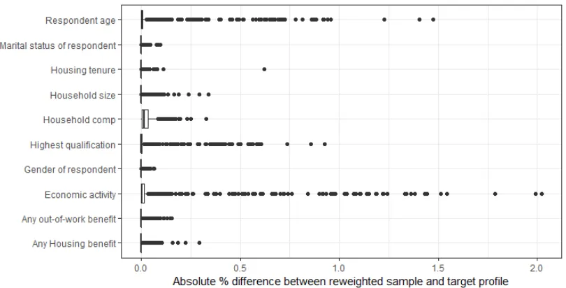
[image:12.612.46.464.310.506.2]

All optimisations converged successfully and so reweighted samples are close to the target LA and PC profile. Average differences are less than 1% across all variables. Figure 2 and Figure 3 demonstrate some variation between areas and between candidate variables, however, differences are all below 3%.

(13)

[image:13.612.50.455.66.272.2]

12

Figure 3: Difference between target PC profile and reweighted samples for each PCNote: dots represent outliers greater than 1.5 times higher than the interquartile range

Overall, these charts indicate that the reweighting succeeds at achieving a close match for most of the constraint variables among most LAs and PCs. For the outliers where this is not achieved, the differences between actual area characteristics and reweighted APMS characteristics are small. The differences appear to be smaller for LAs than for PCs, and are more likely to occur for the following variables: age, highest qualification and economic activity.

Validation against local area proxy indicators

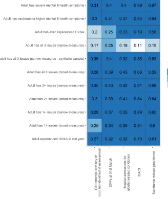
To test the validity of our predictions, we examine whether they correlate as we would expect with other area-level proxy indicators that that were not used in our modelling (because they are not contained in the APMS data). Proxy indicators will generally relate to data on services and service use, which could be rationed and would only relate to the cohort of individuals known to services. As a result, even if the models were ‘perfect’, we would not expect these correlations to be perfect. However we still expect these correlations to be statistically significant and substantial.

Better proxy measures are available at LA level because data on children’s services and other services is collected or reported at that level. We use the following LA-level proxy indicators for validation:

> Income deprivation Affecting Children Index (IDACI) (Source: English indices of deprivation)

> Rate of children referred to children’s services with any of the toxic trio factors identified as a factor at their assessment (Source: CCO internal analysis if the 2017/18 Children In Need census)

> Rates of child protection plans (Source: DfE, Characteristics of children in need 2018)

> Rate of hospital admissions for alcohol related harms amongst adults (source: PHE, Common mental

health disorders prevalence estimates 2016/17)

> Rate of opiate and crack cocaine use (source: PHE, Substance misuse prevalence statistics)

(14)

13

[image:14.612.61.389.113.502.2]

lowest for the outcome “Adult has all 3 issues (narrow measures)”, probably because this outcome is quite rare in the APMS data and therefore more difficult to predict accurately.

Table 6: Correlations between LA proxy indicators and predicted ‘toxic trio’ prevalence rates

Note: figures are Pearson correlations between each proxy indicator and each predicted prevalence rate

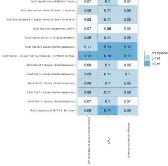
Validating the PC-level predictions is more difficult as less data is published at this smaller geographic level, particularly on the wellbeing of children. The only available proxy indicators we found (which are not used in the modelling) are:

> Income deprivation affecting children (source: House of Commons Library)

> Rates of violent crime (source: CCO internal analysis of LSOA crime figures, aggregated up to PC level using a best-fit lookup)

> GP prevalence of serious mental illness (source: House of Commons Library).

(15)

14

Table 7b shows that the correlations between these proxy indicators and our outcomes measures is much lower, and in some cases not statistically significant. While we would not expect correlations to be perfect for the reasons above, and these proxy indicators are less specific to issues related to the ‘toxic trio’, this

[image:15.612.51.391.189.526.2]

nonetheless indicates a weakness of the PC-level predictions. Of major concern is the fact that the PC-level predictions have very low correlations with IDACI rates (of the order of 0.1), yet the LA-level predictions have very high correlations (as seen in Table 6). This calls into question the quality of implementation of the model for PC-level predictions.

Table 7a: Correlations between PC proxy indicators and predicted ‘toxic trio’ prevalence rates

Note: figures are Pearson correlations between each proxy indicator and each predicted prevalence rate

IDACI-adjusted estimates for parliamentary constituencies

In response to the issues highlighted by Tables 6 and 7a above, we use IDACI scores adjust the PC-level predictions. Ideally, IDACI scores would have been used as a constraint variable in the models, but this was never an option because IDACI is not provided as a variable in the APMS.

(16)

15

Essentially, we stratify the PC-level predictions by IDACI decile, and then renormalise them within IDACI decile (using information from the LA-level predictions). This involves two steps:

1. We estimate the highest and lowest predicted LA-level prevalence rate for each ‘toxic trio outcome’, within each IDACI decile. For example we work out the highest and lowest rate of the ‘all 3’ outcome measure among the 10% most deprived LAs (those with the IDACI scores), and then do this for the second most deprived 10% of LA, and so forth.

2. We rescale our PC-level predictions so that lie between the relevant minima and maxima (conditional on the same IDACI decile) calculated in step 1. For example, a parliamentary constituency that has highest predicted rate of an outcome measure conditional on being in IDACI decile 3, is assigned the highest LA-prediction among LAs in IDACI decile 3. For PCs that lie within the interior of their IDACI decile-specific range – i.e. neither minima nor maxima – the new prediction is imputed through linear interpolation.

Another way to think of this is that it effectively uses the IDACI decile as a ‘match’ variable to link the PC-level and LA-level predictions to each other, with linear interpolation for the actual values themselves.

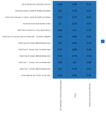
The magnitude of the adjustment is sensitive to the width of the strata, i.e. the type of quantiles used. Here we have used deciles, but wider strata – e.g. IDACI quartiles or quintiles – would have been an option. An important consideration is the need to ensure that the predictions are sufficiently highly correlated with IDACI scores, without overfitting and essentially transforming the predictions into a linear projection of IDACI scores, and while also ensuring reasonable variation between the minimum and maximum within each quantile. Table 7b, below replicates Table 7a after having implemented this IDACI adjustment. Unsurprisingly, the correlations with IDACI scores are much higher – of the order of 0.7 – but, reassuringly, they are not implausibly high (0.9 or above). This also suggests that there is still some variation in predicted prevalence rates even within levels of deprivation. Importantly, the table also shows that correlations with the other two PC-level proxy indicators – GP estimates of mental illness prevalence, and violent and sexual offences – are both significantly higher and always statistically significant.

(17)

[image:17.612.49.400.121.498.2]

16

Table 7b: Correlations between PC proxy indicators and IDACI-adjusted predicted ‘toxic trio’ prevalence rates

Note: figures are Pearson correlations between each proxy indicator and each IDACI-adjusted predicted prevalence rate

Results

Estimated ranges for each ‘toxic trio’ outcome measure

(18)

[image:18.612.48.573.63.307.2]

17

Table 8: Range of central estimates for LA-level and PC-level predictions

Outcome measure Lowest LA rate

(%) Highest LA rate (%)

Adult experienced DV&A in last year 4.9 10.4 Adult has 1+ issues (broad measures) 40.8 54.0 Adult has 1+ issues (narrow measures) 13.9 24.3 Adult has 2+ issues (broad measures) 14.0 24.9 Adult has 2+ issues (narrow measures) 2.9 7.9 Adult has all 3 issues (broad measures) 2.7 5.5 Adult has all 3 issues (narrow measures – synthetic and original

sample) 0.6 1.5

Adult has ever experienced DV&A 21.8 32.5 Adult has moderate or higher mental ill-health symptoms 26.7 39.2 Adult has severe mental ill-health symptoms 9.7 19.0

The full set of central estimate predictions for every LA and every PC is available in spreadsheets. This site also contains interactive maps with map layers showing the predicted local area prevalence of the narrow ‘toxic trio’ measures.

Uncertainty around these estimates

The predictions generated through this modelling come with very wide confidence intervals, especially as they are based on a notional 0.05% sample of adults in each area (see Figures A.1 and A.2 in the Appendix). In fact, we are unable to say that the prevalence rate in any one LA or PC is statistically different from the prevalence rate in any other LA or PC. This is an important caveat to bear in mind, especially in relation to the PC

predictions where the confidence intervals are even wider.

The width of these intervals and the resulting problems for inference indicate that the available data and inputs into for our model have struggled to meet the statistical and computational demands placed on them by the modelling approach. From this we conclude that:

> Additional local area data, especially for parliamentary constituencies, would be useful to improve the model and help to validate the results.

(19)

18

Summary and conclusions

This report sets out a methodology developed by the CCO in order to generate plausible predictions by local area the prevalence of the ‘toxic trio’. It is important to bear in mind the critical challenge for this work – namely, the lack of any such data at a local level – which means that this work is best understood as an innovative and experimental contribution to what is known, rather than a set of definitive answers. With this in mind, our analysis does show that (where data is available) it is possible to generate useful predictions at a local area from national survey data. However the quality of our models, and the resulting predictions, would be massively improved by additional local area data on factors that could be used as constraint variables. Similarly, they would be improved considerably by linking local-level data (such local area deprivation) into national surveys. The model implementations presented in this paper, and results obtained from them, are only optimal given the set of available and feasible constraint variables that currently exists. As this set improves, so would the modelling.

Our LA-level model performs better in the validation checks than the PC-level model, because of this issue. We have good confidence in the plausibility and utility of the LA-level predictions, though further LA-level data would still be useful given the required assumptions.

The PC-level model, heavily restricted because of a lack of feasible constraint variables, performs very poorly in the validation tests. We therefore develop an ex post deprivation-based adjustment in order to ensure that the predictions are more likely to be correlated with deprivation in the way that we would expect. This

adjustment also ensures better consistency between the PC-level and LA-level predictions. Given the use of an

ex post adjustment, we stress that the PC-level predictions remain highly experimental and in need of further

validation based on additional data.

(20)

19

References

Chowdry, H (2018) ‘Estimating the prevalence of the ‘Toxic Trio’: Evidence from the Adult Psychiatric Morbidity Survey’ https://www.childrenscommissioner.gov.uk/wp-content/uploads/2018/07/Vulnerability-Technical-Report-2-Estimating-the-prevalence-of-the-toxic-trio.pdf

Tominitz, M N et al (2008) ‘The geography of smoking in Leeds: estimating individual smoking rates and the implications for the location of stop smoking services’

http://mural.maynoothuniversity.ie/8921/1/JR_smoking%20leeds%202008.pdf

Pryce, R et al. (2017) ‘Estimates of Alcohol Dependence in England based on APMS 2014, including Estimates of Children Living in a Household with an Adult with Alcohol Dependence’

https://www.sheffield.ac.uk/polopoly_fs/1.693546!/file/Estimates_of_Alcohol_Dependence_in_England_base d_on_APMS_2014.pdf

Lunardon N et al (2013) ‘ROSE: A Package for Binary Imbalanced Learning’ https://journal.r-project.org/archive/2014/RJ-2014-008/RJ-2014-008.pdf

(21)

[image:21.792.43.684.92.555.2]