FEA analysis of tractor axle modification

University of Southern Queensland

Faculty of Health, Engineering and Sciences

FEA Analysis Of Tractor Axle Modification

A dissertation submitted by

Richard Sambamo

In fulfilment of the requirements of

ENG4112 Research Project

towards the degree of

ABSTRACT

Agricultural tractor is one of the major and important agriculture implements and the modern heavy agricultural tractors have sophisticated front axles and suspensions. They are also now capable of travelling at speeds of more than 40 km/h. These agricultural tractors are playing an even more important role in the modern Controlled Traffic Farming (CTF) which is being embraced by many Australian farmers. Implementation of CTF however needs the tractors’ front axle to be modified to suit its different and unique farming configuration. The large United States based tractor manufacturers have not been able to satisfy this emerging unique market most likely because of its size and local Australian engineering firms have come up with different front axle modifications custom made to fit particular tractors currently on the market.

The purpose of this research project was to determine the safe loading levels for a modified tractor front axle. The modified tractor axle was for John Deere 8530. Creo 2.0 Parametric and Simulate a modern Finite Element Analysis package was used to complete some robust analysis of the existing product under a wider range of load conditions than are feasible through normal field testing. Manufacturer's CAD data was imported into Creo 2.0 Parametric which was then used to create the 3D model of components and axle. Using the loads calculated from the working weight of the JD8530 and the dynamic loads outlined in Vehicle Standards Bulletin 14 (VSB14), the model was committed to Creo 2.0 Simulate for analysis.

Results of the analysis were processed using the same platform and they indicated a potential problem with component 12 which consistently showed stresses above 300 MPa. These results though were based on worst cases of loadings which are unlikely to occur on the field. It was therefore concluded that the modified axle is safe from stress induced failure if the loadings levels are kept within the capacity of JD8530 tractor.

University of Southern Queensland

Faculty of Health, Engineering and Sciences

ENG4111 AND ENG4112 Research Project

Limitations of Use

The Council of the University of Southern Queensland, its Faculty of Health, Engineering & Sciences, and the staff of the University of Southern Queensland, do not accept any responsibility for the truth, accuracy or completeness of material contained within or associated with this dissertation.

Persons using all or any part of this material do so at their own risk, and not at the risk of the Council of the University of Southern Queensland, its Faculty of Health, Engineering & Sciences or the staffof the University of Southern Queensland.

This dissertation reports an educational exercise and has no purpose or validity beyond this exercise. The sole purpose of the course pair entitled “Research Project” is to contribute to the overall education within the student’s chosen degree program. This document, the

University of Southern Queensland

Faculty of Health, Engineering and Sciences

ENG 4111 AND ENG4112 Research Project

Certi

fication of Dissertation

I certify that the ideas, designs and experimental work, results, analyses and conclusions set out in this dissertation are entirely my own effort, except where otherwise indicated and acknowledged.

I further certify that the work is original and has not been previously submitted for assessment in any other course or institution, except where specifically stated.

Richard Sambamo

Acknowledgements

I would like to thank the project supervisor Chris Snook for his help and guidance on this

research project. His support and facilitation of site visit to the farm is greatly appreciated.

I would also like to thank John Foley for taking his time to drive me down to Denny’s

Engineering and the farm in Allora.Denny’s Engineering are contracted to manufacture the axles. The visit gave me an appreciation of the scope and benefits of the project. He gave

me a lot of invaluable information including background of his innovations and this project.

Table of Contents

Page

Abstract i

Limitations of Use Disclaimer ii

Certification of Dissertation iii

Acknowledgements iv

Table of contents v

List of Figures vi

List of Tables vii

I.0 Introduction

2.0 Background

2.1 Interpreting Client Brief 6

2.2 Project Scope 6

3.0 Literature Review

3.1 Finite Element Analysis 8

3.1.1 Why use Finite Element Analysis 9

3.1.2 Types of FEA software 10

3.1.3 Why use Finite Element Analysis 11

3.2 FEA Validation and Verification 12

3.3 Tractor front axle designs and modifications 13

4.0 Tractor Specifications

4.2 Original front axle configuration 19

4.3 Modified Axle overview and configuration 19

4.3.1 Difference between MK I and MK II Axles designs 20

4.3.2 Material Properties 21

4.3.2.1 Material failure modes 22

4.3.2.2 Factor of Safety Calculations 23

4.4 Related Standards 24

4.4.1 Drop Test 25

4.4.2 VSB 14 Tests 26

5.0 Review of the e-drawings of the modified axle

5.2 Issues with drawings and software. 29

6.0 Parametric model of the modified axle

7.0 FEA Analysis-Structural and Dynamic

7.1 Pre-processing 32

7.1.1 Geometry 32

7.1.5 Boundary conditions 34

7.1.6 Overview of Tests and Loading conditions 35

7.2 Processing 39

7.3 Post Processing/Results 40

8.0 Discussions and Results

42

8.1 Loading case 1 42

8.2 Loading case 2 45

8.3 Loading case 3 48

8.4 Loading case 4 51

8.5 Worst case loading-case 5 53

8.6 Convergence of results 57

9.0 Conclusions and suggestions for future work

9.1 Conclusions 59

9.2 Recommendations 60

9.3 Future Work 61

10.0

References

63

APPENDIX A: Project Specification 67

APPENDIX B: Project Timelines 68

APPENDIX C: 2D drawings, part and assembly models 69

APPENDIX E: Loadings and Constraints 72

APPENDIX F: Risk Assessment 73

APPENDIX G: Factor of Safety Calculations 76

APPENDIX H: Loading Scenarios 78

APPENDIX I: AISI 1020 Steel Mechanical Properties 80

APPENDIX J: Analysis Summary 81

APPENDIX K: Bill of Materials 88

Appendix L: Finite Element Analysis Software Comparison. 90

LIST OF FIGURES

Page

Figure 2.1: Controlled traffic farming in practice. 3

Figure 2.2: John Deere 8530 axle extension. 6

Figure 3.1: Mesh refinements. 10

Figure 3.2: John Deere round bail cotton picker extension. 15

Figure 3.3: Axle extensions. 16

Figure 4.1: JD8530 tractor 17

Figure 4.2: Independent-Link Suspension 17

Figure 4.3: Tractor dimension and weight 18

Figure 4.4: Original John Deere 8350 Tractor axle. 19

Figure 4.5: John Deere 8530 with front modified axle. 19

Figure 4.9: Drop Test Graphical Representation 20

Figure 5.1: Part of Original drawings in e-drawing model viewer. 28

Figure 6.1: Solid Model of Modified Axle sub assembly 30

Figure 6.2: Exploded view of Modified Axle components 31

Figure 6.3: Solid Model of Modified Axle 31

Figure 7.1: Material definition in Creo 2.0 33

Figure 7.2: Finite Element Model of modified Axle 34

Figure 7.3: FE Model of Modified tractor Axle showing constraints and

Loadings 35

Figure 7.4: Weight distribution on front axle 36

Figure 7.5: Loading Conditions and boundary constraints 37

Figure 7.6: Loading case 1: Equal reaction loads 38

Figure 7.7: Coordinate System 39

Figure 7.8: Components Contact issues 40

Figure 7.9: Deformed modified axle model 41

Figure 8.1: Loading case 1 Von Mises Stress plot. 42

Figure 8.2: Identified area of high stress 43

Figure 8.3: Displacement plot for loading case 1. 44

Figure 8.4: Displacement graph for loading case 1. 44

Figure 8.5: Loading case 2 Von Mises Stress plot. 46

Figure 8.6: Identified area of high stress 46

Figure 8.7: Displacement plot for loading case 2. 47

Figure 8.8: Displacement graph for loading case 1. 48

Figure 8.10: Identified area of high stress 49

Figure 8.11: Displacement plot for loading case. 50

Figure 8.12: Displacement plot for loading case 3. 50

Figure 8.13: Loading case 4 Von Mises Stress plot. 51

Figure 8.14: Identified area of high stress 52

Figure 8.15: Displacement plot for loading case 4. 53

Figure 8.16: Displacement graph for loading case 4. 53

Figure 8.17: Loading case 5 Von Mises Stress plot. 54

Figure 8.18: Identified area of high stress 55

Figure 8.19: Displacement plot for loading case 5. 56

Figure 8.20: Displacement graph for loading case 5. 56

Figure 8.21: Convergence of FEA result. 57

Figure B1: Project Timelines. 68

Figure C1: Some examples of modified Axle’s components. 70

Figure C2: Wireframe model of the modified Axle. 70

Figure D.1: John Deere 8530 Tractor information 71

Figure E1: Loadings and constraints on model. 72

Figure H1: Loading Case 1- Normal Reaction loads 78

Figure H2: Loading Case 2 - Bump loads: 4g vertical 78

Figure H3: Loading Case 3–Overturning loads: 4g vertical with 2.5 g

side load 79

LIST OF TABLES

Page

Table 2.1Savings realised by adoption of Controlled Traffic Farming 5

Table 3.1: Comparison of FEA software results 12

Table 4.1: SAE 1020 steel Mechanical Properties of Steel 22

Table 4.2: Factor of Safety Contributions 24

Table 7.1: SAE1020 steel Mechanical Properties of Steel 33

Table 7.2: Tractor axle weight distribution 35

Table 7.3: Loading Scenarios. 38

Table 8.1: Loading case 1. 42

Table 8.2: Computer Memory and Disk Usage 45

Table 8.3: Loading case 2. 45

Table 8.4: Loading case 3. 48

Table 8.5: Loading case 4. 51

Table 8.6: Loading case 5. 54

Table 9.1: Summary of Von Mises stress, displacements and factor of safety 58

Table F1: Risk Matrix 73

Table F2: Project Risk Assessment 75

Table L1: Bill of Materials 89

NOMENCLATURE

Symbol Unit Description

WD Wheel Drive

FW Front Wheel Drive

MFWD Mechanical Front Wheel Drive

I.0 Introduction

An off road tractor is one of the major and important agriculture implements. It is used in most of the agricultural sectors. It is versatile in its uses because of the power built into it and the wide variety of attachments and implements the tractor is able to tow or push. Tractors are playing a more important role in the modern Controlled Traffic Farming (CTF) which is being embraced by some Australian farmers. By the end of 2011, 21 percent of the farmers in Australia had embraced the Controlled Traffic Farming which accounted for six percentage points increase in adoption up from 15 percent in 2008. Adoption of CTF was first done in the early and mid-nineties. These adoption figures were highlighted in the study done by the Grains Research and Development Corporation and released in July 2013.

The Australian Controlled Traffic Association which is responsible for helping and sharing controlled traffic farming techniques at their 2009 annual conference held in Canberra suggested that CTF fifty percent adoption across the farming sector is achievable within ten years with targeted funding. The initial high costs involved in setting up are slowing the take up of CTF and tractor axle modification is certainly one of the costs. The Fact sheet published in July 2013 by the Grains Research and Development Corporation cited that the CTF can improve profitability and sustainability. It also claimed that CTF can improve grain quality and increase the yields by between two to sixteen percent. The uptake of Controlled Traffic Farming can be increased by building confidence in farmers. Farmers have to be convinced that modifications to their expensive farm implements are of high standard and can withstand the structural and dynamic forces involved when farming due to varied field terrain. Modifications to the implements should also be cost competitive. The cost of conversion can be lowered by moving away from the traditional way of design, build prototype and field test. Modern computer technologies are a more cost effective way of designing, perform component behavioural and structural analysis and validation.

farm implements including tractors should be done to high standard and in accordance with relevant standards. This ensures the modifications do not suffer premature failure. This research project seeks to analyse the structural and dynamic implications on a modified front axle for a JD 8530 tractors using Finite Element Analysis. Creo 2.0 Simulate will be mainly used for this analysis. This structural and dynamic analysis will also be done in other available software such ANSYS and Solidworks to compare and validate the results obtained in Creo 2.0 Simulate with time permitting and if such a comparison is necessary.

To simulate the changing terrain of the field, the model of the axle will be subjected to different loading cases and constraints. The Certification load cases as defined for the project will include drop test, Torture Test, The Impact Test, Pit test, Worst load testing and one side impact test. These tests are discussed in more detail under section 4.4 Relevant Standards and Certification Tests.

2.0

Project Background

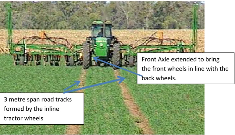
Figure 2.1: Controlled traffic farming in practice.

Controlled Traffic Farming (CTF) is an agricultural system that seeks to minimize the damaging effects of compaction by concentrating wheel traffic to a small area of the field. This is achieved by bringing the front wheels in line with the rear wheels there reducing the overall width of the field area that is being affected by the wheels. The impacted area reduction can be range from 30 to 50 percent depending on the relative sizes of the wheels. The photo in Figure 2.1 shows a narrow distinctive road that has been created due to practice of controlled traffic farming. This ensures that the farm implements use the same tracks all the time. Precision on use of these defined roads have now been improved by incorporation of Global Positioning Systems into the farming system. Farm implements including the tractors are modified to suit different span variations of CTF. Variations in span are 3m, 6m, 9m and 12 metres.

C & C Machining & Engineering, a local engineering company in Toowoomba, Queensland have been involved with widening a great variety of tractors to enable farmers to practice the very effective and increasingly popular controlled traffic farming methods. They claim that they have been modifying the tractors for past 15 years. Controlled farming has certainly been in practice for considerably long time, two decades to be precise and major tractor suppliers such as John Deere and Massey

3 metre span road tracks formed by the inline tractor wheels

Ferguson have not embraced the growing need of this agricultural changing and growing market. Controlled farming seeks to separate the field into farm cropping sections and permanent roads which can be used by all agricultural implements such as combine harvesters and tractors. Extending the front axle brings the front wheels in line with the rear wheels and ensures that they are always on the same track thereby creating some permanent roads on the field. The figure 2.1 above shows the tractor with extended front axle performing controlled traffic farming.

Precision Agriculture (2011) noted that the common spacing or the span of the wheels is normally 3metres and there are other spacing variations such as 9m and 12metres. This effectively means that a 9 and 12 metre span machine can utilise the existing 3 metre roads if the intermediate spacing matches. They also claimed that CTF farming improves the agricultural output. Some studies have been done on the impact of converting to controlled traffic farming on the field yields. Studies carried out by various researchers including Botta, et al (2007), Braunack (2008) and Jensen and Neale (2001) cited in Neale, T (2010) showed that yields are reduced by compaction due to harvest traffic in uncontrolled traffic farming. The yield reductions were considered to range from 15 percent to 30 percent. This translated to losses to the farmers of between $150 to $300 per hectare. The cost of adopting or converting to controlled traffic farming can be recouped within a few years if the losses due to compaction are eradicated by reducing the area in the field exposed to traffic. This ultimately improves the yield and the profit margins.

Details Zero Till CTF Savings Savings

(15% saving) Per Ha CATC Group

Seed ($/ha) 34 30 4 $16,528

Fertiliser ($/ha) * 124 108 16 $66,112

Chemical ($/ha) ** 89 77 12 $49,584

Total 247 215 32 $132,224

The CATC group $ savings relate to 4,132 ha of land being converted to CTF. Fertiliser based on applying 120 kg/ha of urea @ $900/ton.

**

Chemical based on applying 5 l/ha roundup @ $12.5/l & $15/ha for an in-crop spray.

Table 2.1: Savings realised by adoption of CTF Source: (Bowman, K, 2008)

Although uptake of Controlled Farming is on the rise, it is however being slowed down by the fact that modified axles have an unknown risk which the farmers are wary of. Farm implements including the tractor are quite expensive to buy and it is a huge investment for farmers. Any modifications to massive investments such as the tractor have to be therefore done to a high standard that allays any fears the farmers might have. And according to the precision agriculture website, there are obviously some engineering risks with modifying tractors and machinery to wider wheel spacing. The modifications are not normally covered by the original manufacturer’s warranty. Any resultant damage to modified parts including rotating parts such as bearings and drive shaft will have to be repaired at the farmer’s expense. It is for this reason that any modification to the axle has to be done to a high standard and at a reasonable cost which can convince the farmers into taking up the CTF. The modified axle’s susceptibility to breakdowns should therefore be minimised.

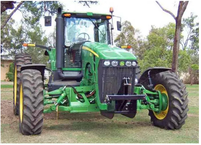
Figure 2.2: John Deere 8530 modified axle extension. (Photo: R Sambamo)

2.1

Interpreting Client Brief

The main objective or emphasis of this research project is to determine the safe loading capacities for the second generation modified axle. The analysis has to be done using modern day computer technology known as Finite Element Analysis (FEA) which has the capacity to simulate designs as in real life situations. The supplied manufacturer's CAD data will be used to build the 3D model of the modified axle. A complete robust analysis of the 3D model of the axle will have to be performed and these tests should cover a wide range of load conditions than are feasible through normal field testing.

2.2 Project Scope

The following is an outline of the scope of this project.

 Relevant literature on axles and different analyses that have been performed

determine the best practices of analysis used in the industry. This will ensure that best and more reliable results are attained.

 Discussion of different loading situations or cases which include:

Drop test, Torture Test, The Impact Test, Pit test, Worst load testing and one side impact test.

 Review of literature related to different loading conditions and testing standards

that might have been used in previous similar studies.

 Review modified axle Cad files.

 Create the 3D models of the axle components and assembly of the components.  Perform static and structural analysis.

 Review the results of the FEA, structural and dynamic analysis.

3.0 Literature Review

The first section of this chapter reviews some literature on various types of finite element analysis software and their underlying theory. This will seek to establish if there is any FEA software that is better than the other one. This of course is in relation to accuracy of the results, ease of use, interface, processing times, computer requirements and the overall cost of setting up.

The second part will review any available literature on tractor or some other heavy duty both on field and off field vehicle axle analysis. This review will give an insight into how other analyses have been done and any flaws in the reports. These will also enable to evaluate the benchmarks against which the tests were performed and any relevant engineering standards applied. Different types of axles will also be reviewed.

3.1

Finite Element Analysis

Finite element analysis (FEA) is defined as a numerical method of solving engineering problems that would otherwise be difficult to solve using analytical methods. Its main uses are quite varied and include calculation of stresses, deflections and displacements in both simple and complex structures. The application of FEA has also been extended to thermal, structural and fluid flow analysis. Despite its application to many different engineering fields the underlying theory is the same.

The structure or component under analysis is basically divided into sections which are more manageable and easy to manipulate. This process is called discretization and according to Logan, the finite element method involves modelling the structure using small interconnected elements called finite elements and a displacement function is associated with each finite element. These elements are then linked either directly or indirectly, to every other element through common or shared interfaces, including nodes and/or boundary lines and/or surfaces. The material’s known stress and strain properties

numerical method gives an estimate result which can be improved by increasing the number of nodes and this obviously results in an even larger set of equations. Computational power of the computer can be utilised to solve these sorts of equations and that is the underlying theory of the FEA software.

3.1.1 Why use Finite Element Analysis

1. It is used as a cost effective way of verifying that a new design or a modification to an existing structure or component will meet the required structural, modal or thermal specifications. The traditional way of manufacturing which involves designing, building a prototype and field testing is expensive because the structural behaviour is not known until the new design has been subjected to field testing. Any subsequent problems that may arise with the new design would mean the prototype will have to be redesigned and modified at a cost. Use of Finite Element Analysis removes the need to build a prototype for testing purposes. The new model is tested and modified accordingly before the component is manufactured or fabricated. FEA analysis is effectively a cost cutting exercise. Behaviour of a component is determined before manufacture and saves on building a prototype which may not be able to meet the specifications.

2. The component or components are loaded and constrained as in real situation. Finite element analysis allows loads simulating the real situation to be applied to the model. Constraints such as displacements, planar and pin can also be applied to mimic actual situations where components can be fixed in various translations or may be joined used a pin joint which allows rotation.

3. The results as to how the component will behave under the suggested loadings and constraints can be processed within short time depending on the complexity of the component and the computer capabilities. A model’s geometry can be easily altered if the results of an analysis are not satisfactory.

5.17% variation from the finite element analysis results. The challenge though is in the interpretation of the FEA results provided that the loadings and constraints have been appropriately applied to a well prepared model. According to Toogood, R, (2012) the results obtained from an FEA modelling depends on the quality of the input data. He says the principles of garbage in garbage out (GIGO) apply when using an FEA package. Results could be improved by either adjusting the model’s meshing or redefining the convergence of the result. The number of elements and nodes in the model can be increased by changing the convergence of the analysis. An example of refinements is shown in the Figure 3.1.

(a)-Course mesh (b)-Intermediate mesh (c)-Fine mesh

Figure 3.1: Mesh refinements. Source: (COSMOL Blog)

The component on the far left in the figure above has a coarse mesh which has been refined in (b) and (c) by increasing the elements and nodes. The nodes are represented by a few dots in (a) and the line connecting the nodes is known as the element.

5. One other advantage in making 3D parametric model and use them for FEA is that it allows fast variations in the model geometry. If the results of FEA are deemed unsatisfactory the analyst can quickly change the geometry in the 3D model by altering the controlling parameters.

3.1.2 Types of FEA software

There is a wide variety of FEA packages on the market and they also vary in their capabilities, pricing and ease of use. A list of FEA packages is shown in Appendix 12. There are 68 FEA software packages that have been compared in the list. They have been compared mainly on their pricing, capabilities, ability to import CAD drawings and types of elements that can be handled. Some of the free software are limited in their capabilities for example FELIPE is only capable of performing four functionalities out of a possible twenty three. There are packages that have extensive capabilities despite being freeware. A package like Elmer is capable of performing around 15 functions out of the possible twenty three. The fact that a package is paid software does not necessarily give it more capabilities than some of the freeware.

Packages are designed for specific applications and it is the ability to perform that particular application that should be considered when deciding which FEA package to use. The applications include the static and structural analysis, Thermal, Computational Fluid dynamics and many more. It is no uncommon to find high cost packages that are quite limited in their applications. These are designed for special applications such as in fluid flow analysis and civil and structural designs. The industry most common packages with a lot of capabilities are ADINA, ANSYS Mechanical NEi/Nastran, Pro/MECHANICA Wildfire 2, COSMOSWorks, COMSOL and Strand 7.

3.1.3 FEA software results comparison

Table 3.1: Comparison of FEA software results Source: (Adams, V)

It was concluded that the results had variations of up to 10% and thus the results from all platforms were reasonably consistent.

3.2

FEA Validation and Verification

The discussion in the above section revolved around how use of different FEA platform influenced the results but the big question is how those results compare to the actual experimental results. The FEA results have to be validated to build some confidence in the outcomes of FEA analysis. An experiment was carried out by Koyuncu, A, Gökler, M, Balkan, T, (2011) to verify the results of FEA on a front axle support for a tractor. Strain gauges were placed on the axle support to measure and calculate the stress under the same loading condition as in the FE Analysis. Results of the experiment were found to have a variance of 7.7% form the FEA results. This basically confirmed that the FEA results can be relied on. MSC/Nastran and Patran finite element analysis packages were used to perform an analysis on the axle support.

measure the stress. They found some that the results of the experiment and the finite element analysis were close and there was a variation of 5.17% in the overall results.

It can therefore be safely concluded that Finite Element Analysis is a reliable and a cost effective way of checking the integrity of designs or modifications. The FEA results correlates favourably with the experimental outcomes. Any platform or the type of software used for an analysis as long as it has the necessary capabilities to perform the particular analysis and the user is competent in its use. Creo 2.0 Parametric and Creo 2.0 Simulate were chosen for the analysis of the modified axle in this project. Creo 2.0 Parametric was used to create the 3D models of the axle components and the complete or assembled model of the axle. The Simulation arm of Creo 2.0 was then used for the finite element analysis of the model. Creo 2.0 Parametric and Simulate although not as popular as the other packages previously discussed was chosen for this project because of its capabilities to perform the required static structural analysis of the modified axle. Other reasons for selecting this particular package include costs and user competency. The package was already on my computer because it had been used in previous courses such computational mechanics so there was no cost involved.

3.3

Tractor front axle designs and modifications

Literature on FEA analysis on tractor axle designs and modifications available is not very extensive and this most probably because of business and property protection issues. The few that are available mainly deal with optimisation of axle designs. An optimisation study was done by Mahanty, D et al and mainly designed an axle with the aim of reducing the weight of the current designs. They managed to reduce the weight of the axle while maintaining the structural and dynamic integrity. ANSYS software was used in this particular analysis and the new designs with reduced weight showed some 15% increase in stresses and displacements which was deemed significantly low. They also managed to reduce the weight by 40 %. This study shows that FEA can be a very effective tool in design and component modification which can ultimately cut costs. 40% reduction is quite significant and depending on the production quantities the savings can also be huge.

back the results from the FEA analysis by performing series of experimental test. In their research León, N concluded that the proposed engineering development process at their DIRONA site proved to be useful in reducing the development time and costs, while maintaining highest product quality and reliability. The software used in this study is SC Patran / MSC Nastran V. 8.0 was used. The axle design or modification can be improved by changing the variables or parameter which includes the materials and the component dimensions which show high levels of stress and strain. Changing some features such as the holes, undercut, radius and their location on a component can also improve the general stress and displacement results. León, N managed to reduce the weight of the axle by 6.8% by changing the design parameters. The stress only increased by 2% which is negligible. According to Aloni, S, Khedkar, S in their comparative analysis of an axle, they also managed to reduce the weight by 10 percent by changing the material from Steel SAE 1020 –Hot Rolled to ASTM A536 (65-45-12) Ductile Iron – Castings. Factor of Safety was improved from 0.7 to 2.4. From these studies it can concluded that modifications and optimisation can be done without compromising the integrity of the component.

Up to this point the literature reviewed did not include the effects of the dynamic forces which are considered significant at high speed. In addition to normal reaction forces on the axle due to the rugged terrain of the field, dynamic forces also have to be considered in the analysis of the behaviour of the axle. Koyuncu, A, Gökler, M, Balkan, T, (2011) outlined the importance of this dynamic feature of the analysis and put it as equivalent to 3g force. The loadings due to dynamic forces are discussed in detail under section 4.4.

3.4 Types of modified tractor axles.

Figure 3.1: John Deere round bail cotton picker extension. (Source: C and C Machining)

In the left photo of Figure 3.1, the original axle enclosed in the blue box has been moved out to accommodate the extension on the left. The axle is a bit complicated than the one shown in the right photo. A provision for the steering rod in the extension creates some manufacturing challenges. Both axles shown in Figure 3.2 result in large moment arms which ultimately put high level stress on the parts joined to the tractor axle or the mounting parts on the wheel end. C and C Machining on their website stated that tubular sections have proved to increase stress on the kingpins on the front axle which may ultimately leads to failure.

Tractors are a huge investment for farmers costing several hundred hundreds of thousands of dollars and conversion costs to controlled traffic farming which may be prohibitive, breakdowns resulting in downtime and added costs is the least of things the farmers have to worry about. This affects the uptake of controlled traffic farming by the farmers for this creates uncertainties around the performance of the modified axle extensions. The traditional method of building a prototype and performing field tests to measure the performance and structural integrity of a design is becoming outdated and it’s not something the farmers want to rely on. Analysis of modified extensions using the now powerful FEA software that has been tested and results validated over the years could boost the confidence of farmers on these modifications. The older tractors without front suspension had to be equipped with a tubular section due to the configuration of the driver train and the suspension. More types of axle extensions are shown below.

Original axle

Axle extension Steering Rod

Figure 3.2: Axle extensions. Source: Larocque, S, 2012 Nuffield Report.

These tractor types shown above do not have a front wheel suspension such as the one incorporated into the JD8530 which enables the front wheels to move up and down in response to the terrain while maintaining the whole tractor level and stable. Detailed discussion of the JD8530 modified axle is in the next chapter.

4.0 Tractor Specifications

John Deere 8530 tractor was manufactured out of United States of America by one of the biggest tractor manufacturers John Deere. It was manufactured from 2006 to 2009.

Figure 4.1: JD8530 tractor. Source (Chris Snook)

Tractor Information or data is in Appendix D. The tractor cost around AU$200 000 to buy second hand and is a huge investment for farmers. Any modification to such equipment has to be of very high standard. The modifications to the front axle of this tractor were complex because of the independent front suspension rams, drive line and the steering rod all of which had to be considered in the axle design. And because of the incorporation of the independent suspension, the tractor is capable of high speeds reaching up to 50 km/h without compromising the comfort of the ride.

Figure 4.2: Independent-Link Suspension Source (John Deere & Chris Snook) Hydraulic cylinder

for suspension

Proximity Sensor

The proximity sensor indicated in Figure 4.2 senses the position in space of pin coupled to the top wishbone and communicates to the control unit which ultimately adjust the wishbones up or down through the hydraulic ram thereby maintaining the level of the tractor. Modifications to the front axle should not compromise such functionalities and its accessories.

4.1 General dimensions and weight.

The Figure 4.3 below shows the overall dimensions of the tractor and the measure that was worth taking note was the operating weight of the tractor. This measure was used in the determination of loads on the tractor axle.

Operating Weight 12156 kg

Wheelbase (D) 3020 mm

Length (A) 5560 mm

Height (C) 3120 mm

4.2 Original front axle configuration

Figure 4.4: Original John Deere 8350 Tractor axle. (Source- John Deere)

The original axle of John Deere 8530 is shown in Figure 4.4 above. The wishbones were basically used to link the block and the wheel hub differential assembly. A hydraulic ram also fixed to the block on one end is attached to the bottom wishbone and can therefore move the block up and down relative to the wheel position.

4.3 Modified Axle overview and configuration

Figure 4.5: John Deere 8530 with front modified axle. (Source-Chris Snook) Hydraulic Ram

Wishbone s

Drive line Transmission

Block

Figure 4.6: Modified John Deere 8350 Tractor axle at close range.

The modified axle is basically a welded and bolted steel block that has been inserted in between the tractor gearbox or transmission block and the wishbones as shown in the figure above. This increases the wheel span of the front axle and increases the performance of the tractor, The new axle is attached to the block using the existing anchor points to which the wishbones were previously attached. The wishbones were moved further out to the new anchoring points on the new axle while still connected to the old existing ones on the wheel side. The axle component parts are discussed in more detail in section 5.

4.3.1 Difference between the two (MK I) and MK II Axles designs

Original Wishbones

Suspension Ram First Generation

Modified Axle Transmission

proved to be a success because it has not failed in operation. It however had some few disadvantages which prompted redesigning or modification. The overall length of the MK I modified axle was a bit longer than required. This resulted in the wheel span being over three metres which was not suitable for the most common controlled traffic farming span. The MK II had to be shortened to resolve this problem. Handling of the first generation (MK I) modified axle is difficult especially when fitting or dismounting onto and off the tractor block. It is a one long block and obviously fitting onto the block poses some challenges. The MK2 is a modification of this first generation axle to rectify any challenges posed MK I. MK I has been basically divided into manageable sections of MK II which can be easily assembled by bolting. A model of the MK II is also shown in Figure 4.7.

(a) Original modified axle-MK I (b) Second generation-MK II model

Figure 4.7: Generation I (MK I) and MK II Axles

Some other crucial modifications have been done which will facilitate easy and quick replacement of parts if for some reason they do fail or get worn out. The parts circled in red in (a) have been modified by drilling bolt holes in them so that they can be bolted onto the main piece instead of being welded.

4.3.2 Material Properties

and a summary of the mechanical properties of the material are shown IN Table 4.1 below. The more detailed list of the material’s properties is in Appendix J.

Table 4.1: SAE 1020 steel Mechanical Properties of Steel

1020 steel has some advantages which make it suitable for use in manufacture of the modified axle and these include welding ability, machinability, heat treatment and low cost. The ability of the steel to be machined is high and it is a requirement for the axle components because most of them have to be machined in some way. The mating surfaces of some components had to be machined to improve the contact area and some had holes for pins bored out and drilled out holes for the bolts.

As can be seen from the first generation modified axle there was some substantial welding done to join most of the components. The SAE 1020 steel used offers high ability for welding which ultimately affect the overall structural integrity or strength of the axle. Convectional or traditional methods of welding can be used in the joining of the SAE 1020 steel parts. This means basic workshop welding equipment which does not need a highly skilled labour can be used in the manufacture of the modified axle. This effectively influences and lowers the cost of manufacturing the axle.

4.3.2.1 Material Failure modes

SAE 1020 is a ductile material and it is likely to show signs of yielding before fracture can take place. If the stress is maintained below the yield stress( ), the steel is in a

position to retain to original shape if the load causing the stress is removed. This phenomenon happens in the elastic region shown in the Figure 4.8 where there is a linear relationship between the stress and strain. Continual application of stress equal or above the yield stress will cause plastic deformation of components which result in

Component Material Density( ) Yield Strength ( ) Tensional Strength ( ) Modulus of elasticity (E) Poisson’s

Ratio ( )

STEEL PLATES

SAE 1020

7800kg/m3 350.00

MPa

420.00 MPa

205,000

left in Figure 4.8 shows the effects of sustained stress above the ultimate stress of the material.

–Yield stress

– Ultimate stress

– Fracture

stress

Figure 4.8: Stress-Strain graph Source (Pennsylvania State University)

The modified axle model will be tested against yield stress which is 350 MPa for the material defined for the model. Stress below this will be deemed to be safe for the model. And stress above the yield stress will be considered unsafe. This although does not result in instant damage but constant exposure to those high stresses cause material fatigue which may ultimately result in failure. Yielding is a probably a good sign of overloading and may prompt replacement or redesign of component.

4.3.2.2 Factor of Safety Calculations

FSmaterial =1.0 If the properties for the material are well known, if they have been experimentally obtained from tests on a specimen known to be identical to the component being designed and v tests representing the loading to be applied

FSmaterial=1.1 If the material properties are known from a handbook or a manufacturer’s values

FSmaterial=1.2–1.4. If the material properties are not well known

Once all contributions are established, the overall factor of safety is calculated as follows:

F.S = FSMATERIALx FSSTRESSx FSGEOMETRYx FSFAILURETHEORYx FSRELIABILITY

The parameters on the right hand side of the equation are estimated using factor of safety guide in Appendix D. If the parameters are well known or defined the factor of safety can be theoretically close to unity but there is always an element of error in areas like workmanship and material. Calculated factor of safety for the modified axle model was calculated as follows.

FSMATERIAL= 1.1

If the material properties are known from a handbook or a manufacturer’s values

FSSTRESS= 1.1 The load is well definedas static orfluctuating

FSGEOMETRY= 1.0

Manufacturing tolerances are average

FSFAILURETHEORY= 1.0 Failure analysis to be used is derived for the state of stress,

FSRELIABILITY= 1.2

The reliability is an average of 92–98%

Table 4.2: Factor of Safety Contributions

A search for specific standards governing the design and testing of tractor axle did not yield results. John Foley, the designer and manufacturer of the JD 8530 front axle extension confirmed that no industry related standards were being used or referred to. Previous studies by Mahanty, D, K Manohar, V, Khomane, B, S, Nayak (2002) on the structural and dynamic analysis of a tractor’s Front Axle however used some test conditions which they called certification tests. Drop test is one of the certification tests

and is discussed in more detail under section

4.4.1

4.4.1 Drop Test

In this test the tractor is driven over a pit which is 762mm deep, 610mm wide and 1500 mm long which is dug on a very hard ground. The maximum dynamic loading component is determined by driving the tractor over the pit at maximum speed of 50km/h. One of the wheels is dropped into the hole and the figure below shows the simplified representation of the scenario at the point when the wheel is in the hole. The tractor is driven from maximum speed to zero speed. The standard distance used for the purposes of these calculations is 1.5 metres.

Figure 4.9: Drop Test Graphical Representation

Calculations of forces to be used in the dynamic analysis for this scenario are as follows

Velocity of the tractor = 50km/h = 13.9 m/s

Acceleration = - where U = initial velocity, S is the distance covered. Mg

R2 R1

= - .

. = - 64.4 m/s

Using F = mass x acceleration

= 631kg x 64.4 m/s

= 40.687 kN force on the front of the axle due to velocity of tractor.

Mass on the front axle is 45% of the total weight of the tractor of 12000 kg = 5400kg.

Reactions R1and R2are equal = (5400/2 x 9.81) = 26.487 kN

The other certification tests which include Torture Test, ‘8’ shaped track test, impact test, pit test and worst load test follow a similar setup as the drop test described above. The difference is in the scenarios which include differing velocity applied and orientation of the axle relative to the field.

4.4.2 VSB 14 Tests

Other studies though have used a different approach to the one adopted by Mahanty, D, K Manohar, V, Khomane, B, S, Nayak (2002) described above. Koyuncu, A & Gökler, M, I & Balkan, T, (2010) in their strength and fatigue analysis for agricultural tractors, they simply used 3g and 2g loading cases to simulate the dynamic loads induced by rugged terrain of the field. VSB14 loading cases used by Krank Engineering are similar to the ones used by Koyuncu, A & Gökler, M, I & Balkan, T, 2010. These are however more detailed and there is some loading cases similarity with those used by Mahanty, D, K Manohar, V, Khomane, B, S, Nayak (2002). Brett Longhurst in his analysis of the front axle of A Holden also used the VBS 14 loading cases. They basically used three loading cases which are specified in Vehicle Standards Bulletin 14, a bulletin produced by department of infrastructure and regional development. The cases though cover vehicles covered by legislation and off road vehicles are not covered in Australian government legislation that is according to the department website. The three loading cases were classified as follows:

1. Loading Case 1: Normal Reaction Loads

2. Loading Case 2: Bump loads: 4g vertical

This simulates the scenario where the vehicle has to drive over a pothole. This

test is similar to the drop loading case used byMahanty, D, K Manohar, V, Khomane, B, S, Nayak (2002) except that the force in this particular case is already defined as 4g vertical. In addition to the calculated reactional forces on the axle due to the weight of the vehicle a vertical force equivalent to four times the weight of the axle also acts in the same direction as the reaction forces. The additional 4g force is applied to one end of the axle. In this loading case the materials ultimate tensile strength is used as the upper limit for this test on the assumption that the critical parameter in this particular test is fracture. The axle in this analysis is allowed to deform due to yielding but not exceeding the fracture limits.

3. Loading Case 3: Overturning loads: 2g vertical with 2.5g side load

Overturning can result in some substantial dynamic loads being imposed on the

axle and to simulate such loads the code recommends that 2g vertical and 2.5g

side or lateral loads be applied. The governing failure mode in this analysis is by

yielding.

4. Loading Case 4: Skid loads: 2g vertical with 1.2g longitudinal

Skid loads or braking loads are applied as combined loadings of2g vertical with 1.2g longitudinal.

5. Loading Case 5: Worst Case Loading

The highest loads in the above four tests are identified for all directions to create a worst case scenario. These are applied that vertical, lateral and horizontally.

5.0 Review of the e-drawings of the modified axle

The client provided an e drawing of the modified axle. The drawings were initially drawn in AutoCAD. E drawings can be viewed using e drawings model viewer in Solidworks and measurements of the components can easily be determined from the drawing using the measure tool in the software. The Figure below shows the some drawings of the component as supplied displayed in the Solidworks e-Drawing Viewer. The drawings could not be modified in the Solidworks e-Drawing Viewer software. Options were considered as to how to import the drawings into Creo 2.0. Redrawing the components one by one using Pro Engineer or Creo Parametric was one option but was deemed to be time consuming. The other alternative considered was using the CAD software and in this case AutoCAD 2014 was used to open the drawing file (DWG).

Figure 5.1: Part of Original drawings in e-drawing model viewer.

5.1 Make 2D drawings of the axle components

opened onto which the highlighted drawing is then pasted. The new drawing is then saved as a DXF file (Drawing eXchange Format). This format enables the files to be opened in other programs other than the AutoCAD. In processing these files into 3D models, they are imported into Creo 2.0 Parametric.

In Creo Parametric, a new 3D part is opened, select the sketch mode and choose a drawing plane. Import the DXF file through the file system under the model toolbar. Under the status (Processing interface data) right click to select the vertex or Csys and accept by clicking the green button. Creo’s default units are English and they were changed to Metric (SI) units before importing the DXF file since the original files were in metric units.

5.2 Issues with drawings and software.

The minimum computer system requirements for running Creo 2.0 on a Windows 7 64-bit operating system are main memory which is normally known as RAM should be at least 4 GB. The memory should be at 3 GB for the Windows 7 32-bit. Installation of academic version of Creo 2.0 was unsuccessful on this system due to PTC registration limitations. Ended up with a student version which has a lot of limitations as far as simulation and structural analysis is concerned. 2D and 3D drawings were however completed using this version of the software.

6.0

3D model of the modified axle

Creo 2.0 Parametric was used to create the 3D model of the modified axle. Some of the modified axle’s 3D components are in Appendix C. The procedure to create an assembly in Creo 2.0 Parametric involves the following steps. The new assembly part is opened and the main part is inserted in the assembly area. The constraints for the main part or the first part to be inserted in the assembly are default constraints. The selected main part for the model was the base plate sub assembly shown in the Figure 6.1 below. The placement or constraint options include coincident, normal, offset angle, parallel and distance. Coincident was used to constrain components with edges, surface, curves and axis which coincide. In the sub assembly in Figure 6.1the holes axis was used to align and constrain the holes in the plates. To complete the placement and mate the plates, the surfaces were constrained using coincident option. All other components were then inserted and constrained appropriately.

Figure 6.1: Solid Model of Modified Axle sub assembly

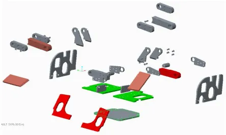
The Figure 6.2 shows the exploded view of Modified Axle components included in the assembly. The names of the components are included in the bill of materials in

Coincident - axis

Figure 6.2: Exploded view of Modified Axle components.

(a) Front view (b) Rear view

Figure 6.3: Solid Model of Modified Axle

7.0 FE Analysis- Static Structural Analysis

As previously stated, the major assumption made for this analysis was that the effect of tyres and hydraulic suspension ram were not considered in the analysis. There are three stages or processes involved in the static and structural analysis of the component. These are namely pre-processing, processing and post processing. In pre-processing the axle model is set up for analysis by converting it into a finite element model by adding and defining some or all of the following finite element model characteristics. The characteristics defined for the model include the geometry of the model, material used in the model and its properties, type of elements, meshing, boundary conditions or constraints and the loads applied. Once the setting up or pre-processing was completed the model was then subjected to a static and structural analysis and this stage of analysis is known as processing. In processing, convergence and outputs are set and these are discussed in more detail in subsection 7.2.--. Post processing was the final stage of analysis where the results of the analysis were analysed, factor of safety calculated and plots of different loading cases and deformed axle model were created.

7.1

Pre-processing

In pre-processing the axle model is set up for analysis by converting it into a finite element model by adding and defining some or all of the following finite element model characteristics. The characteristics which defined the model including the geometry of the model, material used in the model and its properties, type of elements, meshing, boundary conditions or constraints and the loads applied bare discussed in more detail in the subsections below.

7.1.1 Geometry

The 3D solid geometry of the modified axle was created in Creo 2.0 Parametric as shown in the previous chapter. Once imported into Creo Simulate the geometry had to be checked and confirmed.

7.1.3 Material properties of the model.

The material assigned to the model has been discussed in section 4.3.2 Material Properties and the material properties have been included here in Table 7.1 for convenience.

Component Material Density( ) Yield Strength ( ) Tensional Strength ( ) Modulus of elasticity (E) Poisson’s

Ratio ( )

PLATES SAE

1020

7800kg/m3 350.00

MPa 420.00 MPa 205,000 N/mm² 0.3

Table 7.1: SAE1020 steel Mechanical Properties of Steel.

And the following Creo window in Figure 7.1 shows how the material properties in the above table were defined for the model.

Figure 7.1: Material Definition in Creo 2.0

The model’s elements were connected or meshed using meshing for solids known as

tetrahedral elements. The mesh was also automatically generated in the running mode. The difference between a fine meshed and a coarse meshed component is shown in the Figure 7.2 below. Toogood, R (2012) noted that the density of the mesh in Creo does not have a large effect on the final solution of an analysis. The running time of the analysis though can be hugely affected.

(a) Auto meshed (b) Fine meshed

Figure 7.2: Finite Element Model of modified Axle

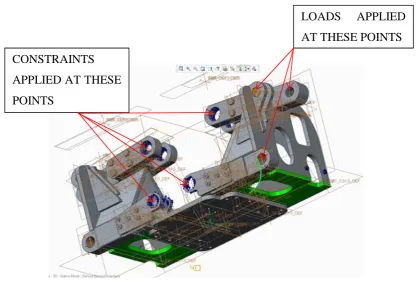
7.1.5 Boundary conditions

Figure 7.3: FE Model of Modified tractor Axle showing constraints and loadings

7.1.6 Overview of Tests and Loading conditions.

Distribution of weight distribution between the front and rear wheels of the tractor had to be considered in evaluation of the actual loadings on the modified front axle. A Canadian government department of Agriculture and development developed a guide on how to evaluate the weight distribution between the front and the rear wheel. The weight distribution depends on type of the tractor especially the type of drive. The table below shows the weight distribution as a percentage for the different types of tractors. These were considered using total ballasted weight or the working weight of the tractors.

Tractor drive type Front Axle Rear Axle

2WD 30% 70%

4WD 55% 45%

FWA 40% 60%

Table 7.2: Tractor axle weight distribution

LOADS APPLIED AT THESE POINTS

John Deere 8530 type of drive is specified as MFWA in the tractor’s data sheet in Appendix 4. The manufacturers sought to differentiate this front wheel drive tractor from one of their previous products which used hydraulics to drive the front wheels. On John Deere 8530 tractor the drive is all mechanical through a gearbox hence the addition of mechanical in Front Wheel Drive. The operating weight of the tractor determined from the information sheet is 12156 kg. Using the 40% to 60% ratio for the FWA drive as a guide for weight distribution for the front axle, the mass acting on the front axle is 4862.4 kg. It has been assumed that the weight due this mass is acting at the centre of the axle as graphically shown in Figure 7.4 below.

4862.4(g) N = 48 kN

l l

RA RB

Figure 7.4: Weight distribution on front axle.

The acceleration due to gravity (g) was assumed to be 9.81m/s2. The reaction RAand RB are equidistant from the centre of the axle. The reactions acting on the wheels are

therefore equal and are half the weight applied at the centre which was 24 kN. The self-weight of the axle was also included in the analysis and using the inspect tool the

volume of the model was determined to be 0.081m3.

Using Density =

Mass = 7800kg/m3x 0.081 m3= 631,8kg.

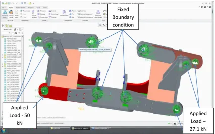
Application of loads and constraints in Creo 2.0 Simulate was performed as follows. On the Creo 2.0 Simulate home screen, bearing load under the Loads section was selected which brought an input window. Inputs such as the surface to be loaded and the magnitude of the force including its direction were defined in the window. The Figure 7.5 shows the loads and constraints and where they have been applied on the model. For the modified axle analysis the central section of the axle which is fixed to the tractor gearbox or transmission block was considered fixed and therefore translations in all directions were restrained. The bearing loads were applied to the outer mounting points of the axle where the wishbones and the hydraulic ram would otherwise be mounted.

Figure 7.5: Loading Conditions and boundary constraints

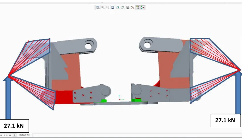
As discussed in section 4.4, the VSB14 loading cases were adopted for static and structural analysis of the modified axle. The Figure below graphically shows how the loads were applied to the ends of the axle. This represents the first test case where the axle was subjected to reactions only at the end due the weight of tractor and modified axle. The 27.1 kN force was applied to each individual mounting point. This was done deliberately so as to create a worst case scenario for the mounting points. A safety

Fixed Boundary condition

Applied Load - 50

kN

feature is thus created and in case the other two mounting points fails then the remaining mount would be capable of safely holding the load.

Figure 7.6: Loading Case 1: Equal reaction loads

Mounting/Wheel A Loads

(kN)

Mounting/Wheel B Loads

(kN)

Loading Case/Test Fx Fy Fz Fx Fy Fz

Test 1 0 27.1 0 0 27.1 0

Test 2 0 27.1 0 0 50.0 0

Test 3 15.5 27.1 0 15.5 38.9 0

Test 4 0 38.9 7.5 0 38.9 7.5

Test 5 (Worst case) 15.5 38.9 7.5 15.5 38.9 7.5 Table 7.3: Loading Scenarios.

The other four loading cases are shown in the table above. The force directions used in

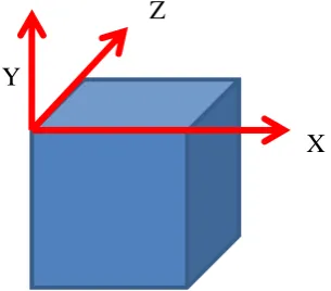
Z

Y

X

Figure 7.7: Coordinate System

7.2

Processing

In the processing stage, the axle model is committed to an analysis by defining the type of analysis, convergence and output file directory in Creo 2.0 Simulate. A new Static and Structural analysis was selected from the file drop down menu and the Static Analysis window came up where constraints and load already applied in the pre-processing stage are selected. Under the convergence tab, the Quick Check method was initially chosen to basically check if there are any errors in the model which may render the analysis insolvable. This initial analysis failed because meshing of some

Figure 7.8: Components Contact issues

The areas on the components that did not have full contact and bondage were modified by introducing bevelled edges as shown in the left section of Figure 7.7. Once the Quick Check analysis was successfully completed the model was subjected to Single-Pass Adaptive method of analysis which is more reliable. An analysis for different loading cases was then run and completed successfully.

7.3 Post Processing/Results

Post processing is the final stage in the analysis where the results obtained from the processing stage are critically analysed evaluated. Creo as some of the post processing software on the market is capable of analysing the results and producing color-coded Stress von Mises plots. It is also capable of sorting, printing, and plotting selected results from a finite element analysis. Some of the routines that can be performed in post processing are sorting element resultant stresses and displacements in order of magnitude, calculation of factor of safety, creating convergence graphs and creation of plots ad graphs

One of the crucial capabilities of post processing software is ability to animate the Contact not complete

behaviour of the model was the outer sections of the model to move in the upward or vertical direction in response to the applied loads. The following plot in Figure 7.9 shows the deformed model of the axle. The deformation has been exaggerated for visual clarity. The results of animation clearly show that the model was correctly constrained.

Figure 7.9: Deformed modified axle model

8.0

Results and Discussions

Results of analysis of different loading cases were analysed for high stress levels and displacements. The results are discussed below for each separate case.

8.1 Loading case 1

In this analysis the following loads shown in table below were applied as discussed under section 7.1 Pre-processing. Vertical loads of 27.1 kN were applied at the outer edges of modified axle.

Mounting/Wheel A Loads

(kN)

Mounting/Wheel B Loads

(kN)

Loading Case/Test Fx Fy Fz Fx Fy Fz

Test 1 0 27.1 0 0 27.1 0

Table 8.1: Loading case 1.

The area of high stress was identified to be the section on the underside of the model at the contact area between the baseplate component 0011RIGHT and component 26R. This localised area of high stress could be a result of some interference of the components which has not been picked up in the quick check analysis due to its small size or nature. In the Simulation diagnostics there was a warning that one or more measures were evaluated at (or close to) results singularities and the results may be inaccurate. This area was ignored as it did not pose any failure and the high stress in this localised area is below the yield stress anyway. Other than this localised area of high stress all other sections of the model have a maximum stress level of around 88 MPa which was way below the yield strength of the material. For this analysis the yield strength had been determined to be the critical parameter. The magnification of the area is shown in Figure 8.2 below.

Figure 8.2: Identified area of high stress

Factor of safety against yield for this analysis was determined as

=

=

=

Factor of safety against fracture for this analysis was determined as Component 19

=

=

=

Displacement results showed a maximum displacement of 0.33mm at the areas colour coded red Displacement plot in Figure 8.3 below. The graphs in Figure 8.4 show the actual areas that were subjected to maximum displacements.

Figure 8.3: Displacement plot for loading case 1.

The graphs in Figure 8.4 show the maximum displacement for the sections indicated by the respective arrows.

Summary of Analysis

Table 8.2: Computer Memory and Disk Usage

8.2

Loading case 2

In this analysis the following loads shown in table below were applied as discussed under section 7.1 Pre-processing. A vertical load of 27.1 kN was applied at one end of modified axle model and another vertical load of 50 kN was applied to the other end to simulate the tractor driving over a hump.

Mounting/Wheel A Loads

(kN)

Mounting/Wheel B Loads

(kN)

Loading Case/Test Fx Fy Fz Fx Fy Fz

Test 2 0 27.1 0 0 50.0 0

Table 8.2: Loading case 2.

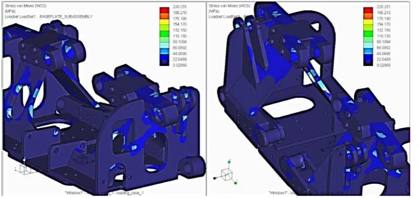
The Figure 8.5 below shows the plots of the stress distribution in the model due to the above applied loading. Different view angles are represented in the stress distribution plots. The maximum stress under these loading conditions was found to be 302 MPa. The controlling mode of failure for this analysis was fracture mode as discussed under section 4.4.

Memory and Disk Usage:

Machine Type: Windows Vista Service Pack 2

RAM Allocation for Solver (megabytes): 512.0

Total Elapsed Time (seconds): 734.99

Total CPU Time (seconds): 357.80

Maximum Memory Usage (kilobytes): 1168864

Figure 8.5: Loading case 2 Von Mises Stress plot.

Factor of safety against yield for this analysis was determined as

=

=

=

Factor of safety against fracture for this analysis was determined as

=

=

=

Displacement results showed a maximum displacement of 0.597mm at the area colour coded red in the displacement plot in Figure 8.7 below. The graph in Figure 8.8 shows the graph and the actual areas that were subjected to maximum displacements.

Figure 8.8: Displacement graph for loading case 1.

8.3

Loading case 3

In this analysis the following loads shown in table below were applied as discussed under section 7.1 Pre-processing. A vertical load of 27.1 kN was applied at one end of the model and 38.9 kN on the other end. A lateral or side load of 15.5 kN was also applied on both ends but in the same direction.

Mounting/Wheel A Loads

(kN)

Mounting/Wheel B Loads

(kN)

Loading Case/Test Fx Fy Fz Fx Fy Fz

Test 3 15.5 27.1 0 15.5 38.9 0

Table 8.3: Loading case 3.

Figure 8.9: Loading case 3 Von Mises Stress plot

There was a localised area of this high stress on the edge of the hole in component 12. The same area showed high stress as in loading case 2. The high stress was due to high loading conditions and geometry of the component. The high stress was on the end where a load of 38.9 kN was applied. The increase in stress levels are was also attributed to additional lateral loading that was applied to the model. Other than this localised area of high stress all other sections of the model have a maximum stress level of around 200 MPa which was below the yield and ultimate strength of the material. For this analysis the yield strength was determined to be the critical parameter.

Figure 8.10 shows the magnified area of high stress.

Factor of safety against yield for this analysis was determined as

=

=

=

Factor of safety against fracture for this analysis was determined as

=

=

=

Displacement