RESEARCH ARTICLE
10.1002/2013JA019464Special Section:
The Causes and Consequences of the Extended Solar Minimum between Solar Cycles 23 and 24
Key Points:
• The source surface height in a PFSS model is a free parameter
• Varying this height during solar mini-mum improves agreement with 1 AU open flux
• The height at minimum is raised 15–30% from the typical 2.5Rs
Correspondence to: W. M. Arden,
Citation:
Arden, W. M., A. A. Norton, and X. Sun (2014), A “breathing” source sur-face for cycles 23 and 24,J. Geophys. Res. Space Physics,119, 1476–1485, doi:10.1002/2013JA019464.
Received 18 SEP 2013 Accepted 1 MAR 2014
Accepted article online 4 MAR 2014 Published online 24 MAR 2014
A “breathing” source surface for cycles 23 and 24
W. M. Arden1, A. A. Norton2, and X. Sun2
1Department of Biological and Physical Sciences, University of Southern Queensland, Toowoomba, Queensland, Australia,
2W. W. Hansen Experimental Physics Laboratory, Stanford University, Stanford, California, USA
Abstract
The potential field source surface (PFSS) model is used to represent the large-scale geometry of the solar coronal magnetic fields. The height of the source surface in this model can be taken as a free parameter. Previous work suggests that varying the source surface height during periods of solar minimum yields better agreement between PFSS models and the measured magnitude of the interplanetary magnetic field (IMF) open flux at 1 AU—in other words, the source surface “breathes” in and out over the course of the solar cycle. We examine the evolution of open flux during all of cycle 23 and the first part of cycle 24 using photospheric magnetic field maps from the Solar and Heliospheric Observatory’s Michelson Doppler Imager and Solar Dynamics Observatory’s Helioseismic and Magnetic Imager instruments. We determine the value of source surface height that provides a best fit to the IMF open flux at 1 AU (using the OMNI 2 data set) for the time period 1996–2012. The canonical 2.5Rssource surface matches the measured IMF open flux during periods of solar maximum but needs to be raised by approximately 15–30% in order to match the measured IMF open flux at the periods of solar minimum.1. Introduction
The extended minimum between solar cycles 23 and 24 gave the solar and geophysics communities an extraordinary opportunity to examine models of the Sun under extreme conditions. Of particular interest to the authors is the accurate measurement and modeling of solar open magnetic flux since this has been shown to be a predictor of solar cycle strength [Feynman, 1982;Wang and Sheeley, 2009]. Solar open flux is also important to the geophysical and space weather communities because it drives the interplanetary magnetic field (IMF), which in turn guides the solar wind and influences the behavior of the Earth’s magneto-sphere. Open magnetic flux has great influence on the large-scale structures in the heliosphere surrounding the Earth.Lockwood[2002] discusses the effects of cosmic rays and total solar irradiance on the Earth’s cli-mate and notes strong correlations among those quantities and total open flux. One proposed physical mechanism is the shielding effect of the heliospheric magnetic field; a more active Sun typically results in a stronger amplitude of open magnetic flux reaching Earth, which in turn lowers the amount of galactic cos-mic rays that can penetrate the Earth’s magnetosphere [Usoskin et al., 2011]. This cosmic ray flux has been linked to terrestrial phenomena as seemingly unrelated as cloud formation [Hanslmeier, 2007, p. 168].
In April 2013, the American Geophysical Union hosted a Chapman Conference devoted specifically to the “Causes and Consequences of the Extended Solar Minimum Between Solar Cycles 23 and 24.” At that confer-ence, we presented results of a preliminary study that modeled the solar corona to calculate total open solar magnetic flux and compared those calculations to estimates of open flux at 1 AU derived from OMNI 2 data [Arden and Norton, 2013].
Raising the source surface height has the opposite effect; there is less open flux, a less curved current sheet, and fewer coronal holes. We ask, do observations sometimes warrant raising or lowering the source surface height? If so, when?
A large body of research has shown a range of appropriate PFSS source surface heights (Rss) from 1.6 to 3.25
solar radii (Rs). The canonical height of the source surface in potential field modeling is reported as 2.5Rs as early as 1983 [Hoeksema et al., 1983]. This height was established because it best reproduced the sector structure of the heliospheric current sheet during solar cycle 21, which included data from 1976 to 1982 and sampled a portion of the rising, maximum, and early declining phases. Specifically, the source surface height range of 2.5–3.0Rswas deemed appropriate because those heights produced high correlations with the measured IMF polarity as observed with the Wilcox Solar Observatory. Near solar maximum, and regions of high activity, other researchers have used a radius of 2.5Rs[Altschuler and Newkirk, 1969;Jackson and
Levine, 1981]. Early work bySchatten and Wilcox[1969] found that 1.6Rswas the best source surface height near minimum. This height was selected to match eclipse photographs showing the field lines becoming radial, the average strength of the radial magnetic field at 1 AU, and the average sector structure of the 1965 solar minimum.Phillips et al.[1994] found a 3.25Rsheight to match the maximum southern extent of the heliospheric current sheet as observed by Ulysses. Research byLee et al.[2011] represented a much needed revisitation of the question of optimum source surface height. Note that our work is focused on using PFSS modeling to estimate the magnitude of the radial field at 1 AU averaged over all latitudes over a Carrington Rotation. We do not attempt to recreate the structure of the heliospheric current sheet, coronal hole areas, or polarity reversals.
Using a PFSS model and consistently treated input data from a single instrument, the relative value of the source surface height that best fits IMF data can be compared at different time periods of the solar cycle or between cycles.Lee et al.[2011] use photospheric field synoptic maps from Mount Wilson Observa-tory (MWO) and find that the values of∼1.9Rsand∼1.8Rsfor the cycles 22 and 23 minimum periods, respectively, produce the best results based on matching coronal hole boundaries and IMF field strength magnitude (not direction). For comparison, Lee et al. also use data from MDI and show that the source sur-face radius of∼1.5Rsproduces better results for cycle 23, rather than∼1.8Rsas suggested from MWO observations. It is understood that PFSS models are considered somewhat less accurate at solar maximum than at minimum; nonetheless, comparison of modeled versus observed B [seeLee et al., 2011, Figure 6d] shows that the best fit for MWO data is given by source surface heights of 1.5 and 1.8Rsfor cycle 23 maxi-mum and minimaxi-mum, respectively. The ultimate conclusion of Lee et al. is thatRssshould be∼1.8–1.9Rsfor the cycle 23 minimum. With respect to the title of their paper, their finding of an appropriate source sur-face height of 1.8Rsat solar minimum is, in fact, lower than the canonical value of 2.5Rsbut higher than the value of 1.5Rsthey find at solar maximum. The case made by Lee et al. is clear and consistent, i.e., the weak polar fields in the cycle 23 minimum lead to weaker global coronal magnetic field and more low latitude coronal holes than were present in the previous minimum. The current work yields similar results in terms of weaker global coronal fields found at the cycle 23 minimum but does not examine the distribution of coronal holes. Note that Lee et al. compare one minimum to another minimum. We compare the solar max-imum time period to the solar minmax-imum. The difference in source surface heights determined in our paper compared to Lee et al. remains unresolved and should be an area for further research.
PFSS models are used to research the physics of open solar magnetic flux (total and spatially distributed), coronal holes, and solar wind outflow [Mackay and Yeates, 2012] as well as heliospheric current sheet struc-ture and corotating interaction regions [Lockwood, 2013, and references therein]. Results byRiley et al.[2006] demonstrate that PFSS models are able to capture the large-scale structure in the solar wind as favorably as more complicated MHD models. Similarly,Owens et al.[2008] found that empirically based models pro-duced the best prediction for near-Earth solar wind metrics compared to MHD models that did not perform as well in the scope of their study. Our choice of PFSS modeling to explore trends in solar open flux was made based on the fact that the community is very familiar with this methodology. In contrast, MHD models show great promise but are still in a stage of testing and development.
At the Chapman Conference, we presented results from a PFSS model developed at Lockheed Martin Solar and Astrophysics Laboratory (LMSAL) bySchrijver and DeRosa[2003]. For this paper, we have added a sec-ond PFSS model developed at Stanford University byZhao and Hoeksema[1993] to our exploration of the relationship between source surface height and the phase of the solar cycle. This paper corroborates and enhances our earlier study.
2. Approach
2.1. General
Our approach was to compute total open magnetic flux at an imaginary source surface (see section 2.3) out-side the corona and compare it to total open flux calculated from magnetic field measurements at 1 AU. The height of the source surface was then adjusted to provide a best match to the measured 1 AU open flux at any given time. This is an adaptation of the process used byLee et al.[2011]; in the present study, data from the Solar and Heliospheric Observatory’s Michelson Doppler Imager (SOHO/MDI) and Solar Dynamics Obser-vatory’s Helioseismic and Magnetic Imager (SDO/HMI) instruments were used as input to two independent PFSS models, and IMF magnetic field data from the OMNI 2 database were used to calculate the open flux at 1 AU. This variation of source surface height can be imagined as an in-and-out “breathing” of the source surface over the course of the solar cycle.
2.2. Magnetograms—The Photospheric Field
The Solar and Heliospheric Observatory’s Michelson Doppler Imager (SOHO/MDI) and Solar Dynamics Observatory’s Helioseismic and Magnetic Imager (SDO/HMI) instruments both produce full-disk line of sight magnetic images of the Sun at a high cadence: once every minute for MDI and once every 12 min (with magnetic field component information) for the HMI vector camera. Calculating total magnetic flux, how-ever, requires knowledge of the field over all longitudes on the Sun, and even a full-disk image can only provide information about the side facing the Earth. Therefore, sets of images are typically combined to pro-duce a synoptic map of the entire Sun over a given period. The two models used are similar except for the following: The LMSAL model uses full-disk magnetograms in a flux-transport model involving differential rotation, meridional flow, and supergranular (diffusive) dispersal, which approximates the evolution of the photospheric field over the entire Sun (not only the visible hemisphere). This yields a continuously evolving picture of the surface field over the whole solar surface at a temporal resolution of 6 h [Schrijver and DeRosa, 2003]. The latest version of this model incorporates integrated polar flux characteristics for an enhanced match to observed flux above 60◦latitude (DeRosa, http://www.lmsal.com/forecast/). The Stanford model, on the other hand, uses a polar field correction based on 2-D spatial and temporal interpolation and a simplified flux-transport function [Sun et al., 2011] and assembles synoptic maps in Carrington Rotation (27 day) format.
Both models take into account the difficulty of measuring magnetic field at the large line of sight projection angles at high solar latitudes [seePetrie, 2012, and references therein]. Estimating these fields is critical for accurate modeling, since they are the sources of stable coronal holes that guide the high-speed solar wind. They are not, however, well observed; techniques of assimilation and interpolation are required to estimate their values. See, for example,Sun et al.[2011] for a discussion of the difficulties and possible solutions to this problem.
The current study used publicly available synoptic maps from LMSAL (see http://www.lmsal.com/forecast for instructions on using the SolarSoft IDL package to download these files) and Stanford University (http:// soi.stanford.edu/magnetic/index6.html). Both sets of maps include polar field correction and are suitable for use as input to the respective PFSS models.
2.3. PFSS—Modeling the Coronal Field
The magnetic fields measured at the photosphere (r=RsunorRs) can be extrapolated to construct a model of the coronal structure. SeeAltschuler and Newkirk[1969] andSchatten and Wilcox[1969] for early deriva-tions andZhao and Hoeksema[1993] andSchrijver and DeRosa[2003] for examples of later developments. Mackay and Yeates[2012] provide an overview of this (and other) models.
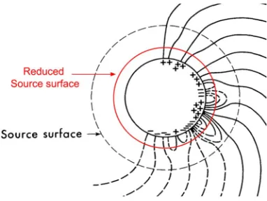
Figure 1.Moving the PFSS source surface affects modeled open flux. Note that lowering the source surface includes more higher-order structure as open flux. Original image is
fromSchatten and Wilcox[1969], and image reproduced is
fromLee et al.[2011].
weather prediction [Arge and Pizzo, 2000]. Models like this are sometimes referred to as Current Sheet Source Surface models [Jiang et al., 2010].
While the corona is known to carry electric cur-rents, these currents are generally not significant on the global scale, except near the heliospheric current sheet. As its name implies, this technique assumes that to be the case below the source surface and does not consider coronal currents. The photospheric field given by magnetograms is used as a lower boundary condition. An imaginary sphere called the source surface (Rss), where the
magnetic field is assumed to be radial only, pro-vides the upper boundary condition. Under these constraints (Rs=B(r,θ,ϕ)andRss=B(r)),∇ ×B⃗=0
and⃗B = −∇Ψ, whereΨis a scalar potential [see Mackay and Yeates, 2012].Ψsatisfies Laplace’s equation:
∇2Ψ =0 (1)
with boundary conditions
𝜕Ψ
𝜕r ||||r=Rs
= −Br(Rs,θ,ϕ) (2)
and
𝜕Ψ
𝜕θ||||r=Rss
= 𝜕Ψ
𝜕ϕ||||r=R
ss
=0. (3)
This equation can be solved using spherical harmonic methods to give the components ofB(r,θ,ϕ)at any point over the rangeRs≤r≤Rss.
The source surface heightRssis commonly taken to be 2.5Rs[Hoeksema et al., 1983]. In fact, though, this is a free parameter in the PFSS model. This fact is critical to our analysis, since it was by varyingRssthat we
observationally constrained the PFSS model to match measured open flux at 1 AU.
The connection between source surface height and open flux is illustrated in Figure 1, adapted byLee et al.[2011] fromSchatten and Wilcox[1969]. Higher spatial orders in the spherical harmonic analysis con-tribute to more complex, but lower, magnetic flux loops. Loops which close beneath the source surface (and therefore do not penetrate it) are not included in the calculation of open flux. As the source surface height is raised, fewer of the higher spatial-order loops penetrate the source surface and open flux decreases. As source surface height is lowered, more of these higher spatial-order loops cross the source surface and open flux increases.
The Sun and its atmosphere exhibit strikingly different behavior at minimum and maximum. This can be observed visually during eclipses or using coronagraph observations of the helmet streamers and other structures in the corona. It is interesting to consider a systematic variation of the source surface height to match the observed conditions of solar maximum and minimum. In practice, a better fit coronal model is likely to benefit space weather operations as well.
Temporal resolution was unfortunately sacrificed in the process of smoothing the output from the LMSAL model to remove the spurious signal from the SOHO roll. In the preparation of this paper, the authors decided to repeat the search for an optimum source surface height using a model that was not affected by this artifact.
One alternative model has been developed at Stanford University. With appropriate correction to include large-scale characteristics of the polar field [Sun et al., 2011], this model yields synoptic maps at an accuracy sufficient for our purposes with a cadence of one Carrington Rotation. Called the “Stanford model” here, it is based on the work ofZhao and Hoeksema[1993] and X. Sun (personal communication, 2013). The ver-sion used for this work is written in Fortran and takes as its input the polar-field-corrected magnetograms available from Stanford (see section 2.2).
As mentioned earlier, results from these two models differ somewhat for reasons explained in section 2.2.
The outputs of a PFSS model include values of the radial B field (Br) over a grid at the source surface. Integra-tion of these values over the sphere gives an estimate of total open flux. In practice, this integraIntegra-tion is a sum of the values weighted by the area of the respective grid elements.
2.4. Open Flux at 1 AU—IMF at Earth
In contrast to the extrapolations of all PFSS models, there is a more direct way to arrive at an estimate of open magnetic flux at 1 AU. Values ofBrare available from the OMNI 2 database (http://omniweb.gsfc.nasa. gov/ow.html). This database was created in 2003 and contains in situ solar wind magnetic field and plasma data from a number of near-Earth spacecraft as well as proton flux and geomagnetic activity indices (e.g.,AE,Dst, and others), all at 1 h intervals. It includes IMF data from November 1963 through July 2013; all three components of the field (Bx,By, andBz) are given in units of nT, in both geocentric solar equatorial and geocentric solar magnetospheric coordinates. We have takenBx, the magnetic field component along the Sun-Earth line, to be equal to the radial field and used data from June 1996 through December 2011 (corre-sponding to the available MDI and HMI data). Daily averages (also found in the OMNI 2 database) were used in our calculations.
Measurements from theUlyssesspacecraft [Smith and Balogh, 1995;Smith, 2008, 2011] show that the radial component of the heliospheric magnetic field is independent of heliospheric latitude. Based on this assumption, the total unsigned flux passing through a sphere with a radius of 1 AU (R1) can be given
simply by
F=4πR21|Br| (4)
as shown byLockwood[2002]. Note that this differs from Lockwood by a factor of 2, since we are concerned with total unsigned, rather than signed, flux.
2.5. Bringing it Together—Optimizing Source Surface Height to Match IMF Observations
The final step in the process was to match the calculated IMF at 1 AU with the results of the PFSS model over the time period of the solar cycle. To do this, the PFSS models were used to calculate time series of open flux at a variety of source surface heights. The IMF open flux at each time period was then compared to these values, which were interpolated as necessary to provide the best fit to the IMF data.
For the LMSAL PFSS model, total open flux was calculated at source surface heights of 1.5, 1.75, 2.0, 2.25, 2.5, 2.75, and 3.0Rs. In order to limit computation to a manageable level, these calculations were performed for 30 day intervals, 4 times per year, over the entire time period. It was found that even a height of 3.0Rswas insufficient to match IMF flux during the cycle 23 minimum; during that period, an additional set of fluxes was calculated at 3.25, 3.5, 3.75, 4.0, and 4.25Rs. The 30 day periods were averaged to a single value per period, giving us four measurements per year, for comparison to IMF open flux.
Figure 2.(top) IMF open flux compared to LMSAL PFSS prediction at 2.5Rs. Both curves are smoothed to 180 days. Black = IMF, blue = LMSAL. Cross-correlation coefficient = 0.911. (bottom) Difference between IMF open flux and open flux calculated from the LMSAL model. Horizontal lines show the root-mean-square (RMS) value of 30 day smoothed, detrended IMF:4.8 ×10²¹Mx.
3. Results
3.1. LMSAL Model
Figure 2 (top) shows total open flux at a 2.5Rssource surface, calculated using the LMSAL PFSS model, compared to IMF open flux from OMNI 2 data. A smoothing window of 180 days is used here on the PFSS curve to minimize the effects of the SOHO roll described earlier; IMF data are also smoothed to 180 days to minimize noise. The two curves are correlated with a cross-correlation coefficient of 0.911.
In order to quantify the times in which a significant difference is observed between the 2.5RsPFSS model data and the IMF data, a value representing a detrended monthly variation was determined. The IMF data were smoothed over 30 days and detrended by subtracting a 1.5 year running average (to remove solar cycle variation and isolate variations on the order of months). The RMS value of this detrended data was then calculated and equaled 4.8 × 10²¹Mx. Figure 2 (bottom) shows the result. The time periods in which
the difference exceeded this value were then determined. This was approximately 23% of the time between July 1996 and December 2011. In only three cases did these periods exceed 6 months in length: the last half of 2002 (9 months), mid-2003 to mid-2004 (9 months), and the cycle 23 minimum of mid-2008 to mid-2009 (11 months, the longest period of difference). These three periods represent anomalies in the rising and maximum phase of cycle 23 and the minimum between cycles 23 and 24 that cannot be reproduced with the usual 2.5Rssource surface height in the PFSS model.
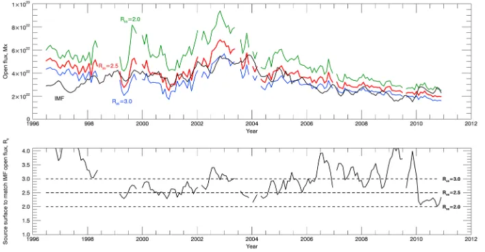
As stated above, open flux was calculated at a number of source surface heights; in Figure 3 (top), the 30 day averages (4 times per year) for the various source surfaces appear as “ladders” through which the IMF flux passes. No smoothing was used in depicting the ladders, and the variation with spacecraft roll angle is evident in the period from mid-2003 until SDO/HMI data replace MDI data in July 2010. In addition, note the added 1 year average bars in 2009; these show the additional flux calculations performed for that period at source surface heights of 3.0–4.25Rs, as discussed earlier.
In Figure 3 (bottom), the optimum source surface height calculated from the LMSAL model is shown. There is general correspondence between the maximum excursions in source surface height and the max-imum differences between IMF and PFSS prediction in Figure 2 (bottom). Note the relatively narrow range of source surface height values (between 2.2 and 2.8Rs) during most of cycle 23 but the significant rise in height to a maximum of 3.3Rsduring the cycle 23 minimum. The average source surface height that matched the OMNI IMF open flux during the cycle 23 minimum (taken to be the time period from the beginning of 2007 to June 2009) is 2.88Rs. This represents a 15% rise in the source surface height used at solar minimum.
3.2. Stanford Model
Figure 3.(top) IMF open flux compared to 30 day average values for source surfaces from 2.0Rsto 4.25Rs, predicted from the LMSAL PFSS model. (bottom) Optimum source surface height matching IMF open flux, based on LMSAL model.
and IMF values at the start of cycle 23. This is due in part to overestimates of the polar field in the synop-tic maps. The scheme [Sun et al., 2011] uses better-observed data each year (September for the Northern Hemisphere, March for the Southern Hemisphere) to constrain the polar values. Prior to the first
September/March observations, however, the values are extrapolated; this creates large uncertainties early in the model.
A consistently higher value from the PFSS model can also be seen during the later declining phase of the cycle and the minimum. Missing values in the PFSS model are primarily the result of the “SOHO vacation” around CR1935-1945 (April 1998 to January 1999). Missing data also exist during other brief periods due to incomplete source magnetograms on which the PFSS extrapolations were based. Linear interpolation was performed to fill in missing data, and the data were smoothed to six Carrington Rotations (approximately 164 days) in order to compare with the LMSAL data. With this smoothing, cross correlation with similarly smoothed IMF data yielded a correlation coefficient of 0.726. The same criteria used to quantify variations between the LMSAL model and IMF data were applied to the Stanford model and IMF data. Periods longer than 6 months in which the difference between the CR-smoothed IMF data and the Stanford model predic-tions exceeded 4.8 ×10²¹Mx occurred from July 1996 (the start of the data) to June 1998, from mid-2002
to mid-2003, from mid-2006 to late 2006, and from mid-2008 to mid-2009 (the cycle 23 minimum).
[image:7.612.200.550.521.699.2]Figure 5.(top) IMF open flux compared to Stanford model predictions for source surfaces from 2.0Rsto 3.0Rs. Black curve = IMF; green = 2.0Rs; red = 2.5Rs; blue = 3.0Rs. (bottom) Optimum source surface height matching IMF open flux, based on Stanford model, smoothed over three Carrington Rotations. Maximum source surface height calculated was 4Rs.
Figure 4 (bottom) shows the differences graphically. For 74.1% of the CRs for which we had good data, the difference between IMF open flux and Stanford model open flux was greater than the detrended RMS value of the IMF flux.
Figure 5 (top) depicts IMF open flux versus source surface heights from 2.0 to 3.0Rsand may be compared to the LMSAL model predictions of Figure 3 (top). This plot reveals that for the Stanford model, the IMF flux was generally higher than flux calculated for 3.0Rsexcept for the cycles 22–23 minimum and the declining phase of cycle 23. We therefore anticipated that the optimum source surface height would lie below 3.0Rsin the middle part of the cycle, rising (to give less open flux) in the declining phase. During the rising phase of cycle 23, there was a dramatic difference between the model and the IMF flux. With these results, it became evident that further calculations would be needed to determine optimum source surface height for some time periods. These calculations were performed to cover the parts of cycle 23 where the IMF open flux was clearly lower than the calculated model; see, for example, CR 2040-2060 (February 2006 to August 2007) and CR 2075-2095 (October 2008 to March 2010). In these periods, additional source surface heights as high as 4.0Rswere computed.
In Figure 5 (bottom), the calculated optimum source surface height based on the Stanford model is shown. Overall, this confirms the above expectation. Note that the source surface height is far too high for the rising phase of cycle 23, generally lies in the region between 2.0 and 3.0Rsfor the middle third of the cycle and then rises over the declining phase before it declines as cycle 24 begins. The average value of source surface height over the cycle 23 minimum is 3.28, a 30% increase from the typical value of 2.5Rs.
4. Discussion
Figure 6 shows total unsigned open flux results from both PFSS models and OMNI/IMF data. For this com-parison, all three curves were smoothed; the IMF and LMSAL data to 180 days and the Stanford data to six Carrington Rotations (approximately 164 days). The three curves generally track; as mentioned earlier, the cross-correlation coefficients were 0.911 between IMF and LMSAL and 0.726 between IMF and Stanford. Dis-parities among them, however, gave clues to the regions in which varying the source surface height would give a better fit.
Figure 6.Total unsigned open flux as calculated by LMSAL and Stanford models, compared to calculated values based on OMNI/IMF data. Source surface height is fixed at 2.5Rsfor both PFSS models.
A higher source surface height, for instance, also gives rise to a less curved current sheet—which does not agree well with observations.
The original premise of this work was that varying source surface height in the PFSS model could be used to more accurately describe the Sun’s open flux when compared to IMF measurements at 1 AU. Two different PFSS models were used to test this hypothesis. Over the last two thirds of cycle 23, both models were con-sistent in supporting our hypothesis; the canonical source surface height of 2.5Rsprovides good results for the middle third of the cycle (corresponding to solar maximum), and increasing the height improves the fit to IMF open flux in the declining phase of the cycle. The average source surface height that best matches IMF open flux observed in the OMNI database during cycle 23 minimum (2007 to June 2009) is 2.88 from the LMSAL model and 3.28 from the Stanford model. This represents a∼15%rise in the source surface height at minimum for the LMSAL model and a∼30%rise for the Stanford model. Both models showed a decrease in height as cycle 24 begins.
The agreement was not as good during the rising phase of cycle 23. The LMSAL model produced a source surface height in the range around 2.5Rs, but the Stanford model yielded very high (>4.0) source surface heights. The likely reason for this is outlined in section 3.2.
5. Conclusions and Summary
The extended solar maximum at the end of cycle 23 was examined in the context of the entire cycle and the beginning of cycle 24. Total unsigned open magnetic flux was estimated using two different PFSS mod-els and compared to calculated open flux at 1 AU based on in situ IMF measurements from the OMNI 2 database. Source surface heights in both models were optimized to match measured flux.
The findings of this study can be summarized as follows:
1. Both PFSS models did a reasonable job of estimating IMF open flux over the time period of cycle 23 and the start of 24 using the typical source surface height of 2.5Rs, with correlation coefficients of 0.73 (Stanford) and 0.91 (LMSAL).
2. Differences between modeled (PFSS) open flux (with a source surface height of 2.5Rs) and measured (IMF) open flux were on the order of the RMS value of IMF open flux after 30 day smoothing and detrending. 3. Altering the source surface height yielded more precise matching of the PFSS calculated open flux to
measured IMF open flux. Calculating open flux over a range of source surface heights enabled the use of interpolation to find the best match over the solar cycle.
In summary, this study confirms the use of PFSS modeling as a method of describing total solar open mag-netic flux over the duration of the solar cycle. The significance of the current work is the improvement of a standard method of modeling the coronal magnetic field, with the ultimate goal of enabling more conve-nient use of PFSS models in solar cycle and space weather prediction. It is believed that refinements such as this will enhance the value of these models as predictors of solar cycle behavior and the resulting effects.
References
Altschuler, M. D., and G. Newkirk Jr. (1969), Magnetic fields and the structure of the solar corona I: Methods of calculating coronal fields, Sol. Phys.,9, 131–149.
Arden, W. M., and A. A. Norton (2013), A “breathing” source surface for cycle 23/24, inCauses and Consequences of the Extended Solar Minimum Between Solar Cycles 23 and 24, AGU, Washington, D. C.
Arge, C. N., and V. J. Pizzo (2000), Improvement in the prediction of solar wind conditions using near-real time solar magnetic field updates,J. Geophys. Res.,105, 10,465–10,479.
Feynman, J. (1982), Geomagnetic and solar wind cycles, 1900–1975,J. Geophys. Res.,87, 6153–6162. Hanslmeier, A. (2007),The Sun and Space Weather, 2nd ed., Springer, Dordrecht, Netherlands.
Hoeksema, J. T., J. M. Wilcox, and P. H. Scherrer (1983), The structure of the heliospheric current sheet: 1978–1982,J. Geophys. Res.,88, 9910–9918.
Jackson, B. V., and R. H. Levine (1981), A comparison of type III metric radio bursts and global solar potential field models,Sol. Phys.,73, 183–190.
Jiang, J., R. Cameron, D. Schmitt, and M. Schussler (2010), Modeling the Sun’s open magnetic flux and the heliospheric current sheet, Astrophys. J.,709, 301–307.
Lee, C. O., J. G. Luhmann, J. T. Hoeksema, X. Sun, C. N. Arge, and I. de Pater (2011), Coronal field opens at lower height during the solar cycles 22 and 23 minimum periods: IMF comparison suggests the source surface should be lowered,Sol. Phys.,269, 367–388. Lockwood, M. (2002), Long-term variations in the open solar flux and possible links to Earth’s climate,From Solar Min to Max: Half a Solar
Cycle With SOHO,ESA SP-508 SOHO 11 Symposium, Davos, Switzerland.
Lockwood, M. (2013), Reconstruction and prediction of variations in the open solar magnetic flux and interplanetary conditions,Living Rev. Sol. Phys.,10, 4–88.
Mackay, D. H., and A. R. Yeates (2012), The Sun’s global photospheric and coronal magnetic fields: Observations and models,Living Rev. Sol. Phys.,9, 6–64.
Owens, M. J., H. E. Spence, S. McGregor, W. J. Hughes, J. M. Quinn, C. N. Arge, P. Riley, J. Linker, and D. Odstrcil (2008), Metrics for solar wind prediction models: Comparison of empirical, hybrid, and physics-based schemes with 8 years of L1 observations,Space Weather, 6, S08001, doi:10.1029/2007SW000380.
Petrie, G. J. D. (2012), Evolution of active and polar photospheric magnetic fields during the rise of cycle 24 compared to previous cycles, Sol. Phys.,281, 577–598.
Phillips, J. L., A. Balogh, S. J. Bame, B. E. Goldstein, J. T. Gosling, J. T. Hoeksema, D. J. McComas, M. Neugebauer, N. R. Sheeley Jr., and Y. M. Wang (1994), Ulysses at 50◦south: Constant immersion in the high-speed solar wind,Geophys. Res. Lett.,21, 1105–1108. Riley, P., J. A. Linker, Z. Mikic, R. Lionello, S. A. Ledvina, and J. G. Luhmann (2006), A comparison between global solar
magnetohydrody-namic and potential field source surface model results,Astrophys. J.,653, 1510–1516.
Schatten, K. H., and J. M. Wilcox (1969), A model of interplanetary and coronal magnetic fields,Sol. Phys.,6, 442–455. Schrijver, C. J., and M. L. DeRosa (2003), Photospheric and heliospheric magnetic fields,Sol. Phys.,212, 165–200. Smith, E. J., and A. Balogh (1995), Ulysses observations of the radial magnetic field,Geophys. Res. Lett.,22, 3317–3320.
Smith, E. J. (2008), The global heliospheric magnetic field, inThe Heliosphere Through the Solar Activity Cycle, edited by A. Balogh, L. J. Lanzerotti, and S. T. Seuss, pp. 79–144, Praxis, Chichester, U. K.
Smith, E. J. (2011), Solar cycle evolution of the heliospheric magnetic field: The Ulysses legacy,J. Atmos. Sol. Terr. Phys.,73, 277–289. Sun, X., Y. Liu, J. T. Hoeksema, K. Hayashi, and X. Zhao (2011), A new method for polar field interpolation,Sol. Phys.,270, 9–22. Usoskin, I. G., G. A. Bazilevskaya, and G. A. Kovaltsov (2011), Solar modulation parameter for cosmic rays since 1936 reconstructed from
ground-based neutron monitors and ionization chambers,J. Geophys. Res.,116, A02104, doi:10.1029/2010JA016105. Wang, Y.-M., and N. R. Sheeley (2009), Understanding the geomagnetic precursor of the solar cycle,Astrophys. J. Lett.,694, L11. Zhao, X., and J. T. Hoeksema (1993), Unique determination of model coronal magnetic fields using photospheric observations,Sol. Phys.,
143, 41–48. Acknowledgments
The authors would like to thank the referees for their constructive and helpful comments. The authors wish to acknowledge Xuepu Zhao and J. Todd Hoeksema of Stanford University and Marc DeRosa of LMSAL for their assistance in the research that led to this paper. The OMNI data were obtained from the GSFC/SPDF OMNI-Web interface at http://omniweb.gsfc. nasa.gov.