A note on dissipative particle dynamics (DPD) modelling of simple fluids

A Note on Dissipative Particle Dynamics (DPD)

Modelling of Simple Fluids

N. Phan-Thien

, N. Mai-Duy

and T.Y.N. Nguyen

1

Department of Mechanical Engineering, Faculty of Engineering,

National University of Singapore, 9 Engineering Drive 1, 117575, Singapore,

2

Computational Engineering and Science Research Centre,

School of Mechanical and Electrical Engineering,

University of Southern Queensland, Toowoomba, QLD 4350, Australia.

Submitted to

Computers & Fluids

, June/2018; revised, August/2018

ABSTRACT: In this paper, we show that a Dissipative Particle Dynamics (DPD) model of

a viscous Newtonian fluid may actually produce a linear viscoelastic fluid. We demonstrate

that a single set of DPD particles can be used to model a linear viscoelastic fluid with its

physical parameters, namely the dynamical viscosity and the relaxation time in its memory

kernel, determined from the DPD system at equilibrium. The emphasis of this study is placed

on (i) the estimation of the linear viscoelastic effect from the standard parameter choice;

and (ii) the investigation of the dependence of the DPD transport properties on the length

and time scales, which are introduced from the physical phenomenon under examination.

Transverse-current auto-correlation functions (TCAF) in Fourier space are employed to study

the effects of the length scale, while analytic expressions of the shear stress in a simple small

amplitude oscillatory shear flow are utilised to study the effects of the time scale. A direct

mechanism for imposing the particle diffusion time and fluid viscosity in the hydrodynamic

limit on the DPD system is also proposed.

Keywords: Dissipative particle dynamics (DPD); simple fluids; generalised hydrodynamics;

Newtonian fluids; linear viscoelastic fluids

∗_{Corresponding author E-mail: [email protected], Telephone 46312748, Fax}

1

Introduction

In the dissipative particle dynamics (DPD) (e.g. [1]), the fluid is modelled by a system of

particles undergoing their Newton 2nd law motions

mi¨ri =miv˙i = N

X

j=1,j6=i

(Fij,C +Fij,D+Fij,R), (1)

where N is the number of particles, mi, ri and vi the mass, position vector and velocity

vector of a particle i, respectively, and Fij,C, Fij,D and Fij,R the conservative, dissipative

and random forces, respectively,

Fij,C =aijwCeij, (2)

Fij,D =−γwDeij ·vijeij, (3)

Fij,R=σwRθijeij, wR =√wD, σ=

p

2γkBT , (4)

in which aij, γ and σ are the amplitudes, and wC, wD and wR, the weighting functions,

with eij = rij/rij the unit vector from particle j to particle i (rij = ri −rj, rij = |rij|),

vij =vi−vj the relative velocity vector,kBT the Boltzmann temperature andθij a Gaussian

white noise. It is noted that the characteristics of the random force are defined by the

fluctuation-dissipation theorem. In practice, one usually employs the weighting functions of

the form

wD =

1₋ r

rc

s

, (5)

wC =

1₋ r

rc

, (6)

where s is a positive value (s = 2 and s= 1/2: standard and modified values, respectively)

and rc the cut-off radius. The DPD input parameters include s, aij, σ, kBT, m, rc and the

particle density n.

mean - in that sense it is a bottom up approach to solving NS equations. It requires no prior

specification of the constitutive relation for the fluid - the stress-strain rate relation is also

obtained as a part of the solution procedure. It has been shown that, for preceding standard

descriptions of the DPD interaction parameters, the DPD system is actually a Newtonian

fluid on a long-time average [1]. In this work, we explore the generalised hydrodynamic

regime of a DPD fluid that is defined by equations (1)-(6), where typical length scales

include the interaction range rc and the dynamic correlation length l0 defined asl0 =v0t0 in

which v0 and t0 are, respectively, the typical thermal velocity and collision time (or kinetic

time) [1]

v0 = r

kBT

m , (7)

t0 =

1

ω0

, ω0 =

n[wD]γ

3m , [wD] = 4πr

3

c

1 1 +s −

2 2 +s +

1 3 +s

. (8)

The classification of dynamic regimes in DPD can be based on the two length scales, rc and

l0: “particle” regime when rc < l0 and “collective” regime when rc > l0. In this work, the

focus is on a collective regime. Note that if one takes n =_{3,4_}, rc = 1,m = 1, σ = 3 and

kBT = 1 (commonly used input values), then the above estimates yieldl0 ={0.5305,0.3979}

fors = 2 (standard DPD fluids) andl0 ={0.1161,0.087}fors= 1/2 (modified DPD fluids),

all less than rc = 1.

Let λ be the wavelength (k = 2π/λ is the wave number) of a perturbation in the

hydrody-namics, which can be regarded as the length scale on which the physical phenomena under

examination occur. On the other hand, the correlation length l0 forms a scale on which the

DPD transport coefficients are defined. Ask _→0 and the observation time scale is large, the

system behaves like a continuum (the NS equations/hydrodynamics limit). At finite k, the

system can be described by a linearised form of the NS equations, where local deviations of

the macroscopic variables (the number density and momentum density) from their average

values are assumed to be small. As discussed in [2], a standard hydrodynamic regime occurs

on the range l0 < rc < λ while a mesoscopic hydrodynamic regime on l0 < λ < rc. In

addition, there is a smooth transition between these two hydrodynamic regimes, which

mesoscopic hydrodynamics and thus can be probed by considering linearised NS equations

induced by perturbations. The transport coefficients are now functions ofk, and their values

atk = 0 can be estimated through extrapolation. The regime of generalised hydrodynamics

is particularly relevant in the simulation of complex fluids such as colloidal suspensions. In

practice, an effective way to predict the DPD transport coefficients over a wide range of k

is to employ the transverse-current autocorrelation functions (TCAF) in Fourier space [1,2].

Letωbe a characteristic frequency (T = 1/ωis a characteristic time). Assume that our

(non-Newtonian) fluid in question has a characteristic time scale λt. If T ≫ λt, the observation

time scale is large and the material responds like a fluid; otherwise, one may have a solid-like

response. For a linear viscoelastic fluid, the stress at the current time is dependent not only

on the current strain rate but also the past strain rate; in 1D,

σ(t) =

Z γ(t)

γ(−∞)

G(t₋t′_)dγ(t′_{) =}

Z t

−∞

G(t₋t′_{) ˙γdt}′_{, (9)}

where ˙γ is the shear rate (γ is the shear strain) and G is a decreasing function of time, the

relaxation modulus. In the case of a simple shear flow, the stress analysis can be done in an

exact manner. One can utilise its analytic solution to examine the effects of the frequency

on the DPD transport properties.

One particular concern here is how to make a direct link between the fluid physical

parame-ters and the (input) DPD parameparame-ters. We attempt to derive, by means of kinetic theory [1]

and by using generalised forms of the dissipative weighting function, the relation between

the particle diffusion time and the viscosity of the fluid (at the hydrodynamic limit), and the

DPD parameters. The resultant analytic expressions allow one to specify these two physical

parameters as the input parameters.

The remainder of the paper is organised as follows. In Sections 2 and 3, brief reviews of

TCAF and analytic expressions of the shear stress in a simple small amplitude oscillatory

shear flow are respectively given. In Section 4, we investigate the dependence of the DPD

the hydrodynamic limit on the DPD system, and quantify the linear viscoelastic effect from

the standard parameter choice. Numerical experiments are presented in Section 6. Section

7 provides some concluding remarks.

2

Time current autocorrelation functions

The current density is given by

j(r, t) = N

X

j=1

vjδ(r−rj(t)), (10)

where N is the number of particles and subscripts j denote particle number. Since there

is no overall motion, _hj(r, t)_i = 0 (< _· > denoted the average operation). Note that j(r, t)

is the macroscopic (hydrodynamic) variable and v the microscopic variable. The Fourier

transformation of (10) is

J(k, t) = Z

drexp(ik_·r)j(r, t) = X j

vj(t) exp(ik·rj(t)). (11)

The spatial correlation function is defined as [3,4]

Cαβ(k, t) = k2

NhJα(−k,0)Jβ(k, t)i, (12)

where α and β denote Cartesian indices.

For an isotropic fluid, the correlation function (12) depends only on the magnitude of kand

one can decompose it into the longitudinal (k) and transverse (⊥) components relative to k

as

Cαβ(k, t) = kαkβ

k2 Ck(k, t) +

δαβ − kαkβ

k2

where δαβ is the Kronecker delta, and

C⊥(k, t) =

k2

NhJ⊥(−k,0)J⊥(k, t)i, (14) Ck(k, t) =

k2

NhJk(−k,0)Jk(k, t)i. (15)

3

Analytic solutions for simple shear flows of linear

viscoelastic fluids

Here we recall some terminologies by considering a small amplitude oscillatory shear flow of

a viscoelastic fluid. The flow is generated between two parallel plates separated by a distance

h. The bottom plate is fixed while the top plate is sinusoidally displaced by δsin(ωt) with

δ _≪h being the small amplitude displacement in the x direction. The top plate velocity is

U(t) =δωcosωt. (16)

The shear rate and the shear strain experienced by the fluid are, respectively,

˙

γ(t) = δ

hωcosωt= ˙γ0cosωt, (17)

γ(t) = δ

hsinωt=γ0sinωt, γ0 = δ

h ≪1, γ˙0 =ωγ0. (18)

For a linear viscoelastic fluid at any arbitrary amplitude δ, or for any viscoelastic fluid at a

small enough amplitude δ, the only non-zero component of the stress is the shear stress

τxy =

Z t

−∞

G(t₋t′)∂ux(y, t

′₎

∂y dt

′ ₌

Z t

−∞

G(t₋t′) ˙γ0cosωt′dt′,

=

Z ∞

0

˙

γ0G(s) cosω(t−s)ds,

=

Z ∞

0

˙

γ0G(s)[cosωtcosωs+ sinωtsinωs]ds,

=G′(ω)γ0sinωt+η′(ω) ˙γ0cosωt,

where G′_{(ω) is the storage modulus and η}′_{(ω) is dynamic viscosity; they are related to the}

relaxation modulus G(t) by

G′(ω) =

Z ∞

0

ωG(s) sin(ωs)ds, (20)

η′(ω) =

Z ∞

0

G(s) cos(ωs)ds. (21)

By rewriting (19) as

τxy =G′(ω)γ0sinωt+η′(ω) ˙γ0sin(

π

2 +ωt), (22)

the shear stress is shown to have the same phase as the applied strain for the elastic part,

but π/2) out of phase from the applied strain for the viscous part. All of the foregoing are

familiar results in continuum mechanics (e.g. [5]).

4

Generalised DPD transport coefficients

The conservation laws for the mass density ρ(r, t) and momentum density mu(r, t) in the

continuum description read

∂ρ(r, t)

∂t +∇ ·(ρ(r, t)u(r, t)) = 0, (23) ∂

∂tρ(r, t)u(r, t) +u(r, t)· ∇(ρ(r, t)u(r, t)) +∇ ·σ(r, t) =0, (24)

where σ is a stress tensor.

4.1

Newtonian fluids

In this case, the stress tensor is given by

σαβ(r, t) =δαβp(r, t)−η

∂uα(r, t) ∂rβ

+∂uβ(r, t)

∂rα

−δαβ∇ ·u(r, t)

ηB− 2 3η

where p is the local pressure, η the shear viscosity and ηB the bulk viscosity.

Without applied external forces, one has _hu(r, t)_i= 0. Assume that local deviations of the

hydrodynamic variables from their average values are small, the variables in (23), (24) and

(25) can be expressed as [3,4]

n(r, t) = n+δn(r, t)_≈n, (26)

u(r, t) = _hu(r, t)_i+δu(r, t) =δu(r, t), (27)

ρu(r, t) = m(n+δn(r, t)) (_hu(r, t)_i+δu(r, t))_≈mnδu(r, t) =mnu(r, t) =ρj(r, t), (28)

where high-order terms have been ignored and n is the equilibrium number density of the

system. At equilibrium, the variables < δn(r, t)> and < δu(r, t)> disappear.

Making use of (25) and (26)-(28), the conservation equations (23) and (24) reduce to the

following linear form of the Navier-Stokes equation

∂δρ(r, t)

∂t +∇ ·ρj(r, t) = 0, (29) ∂j(r, t)

∂t +

1

ρ∇p(r, t)− η ρ∇

2_{j(r, t)}

− 1_ρ

ηB+ 1 3η

∇∇ ·j(r, t) = 0. (30)

In Fourier space, they become

∂δρ(k, t)

∂t +ik·ρJ(k, t) = 0, (31) ∂J(k, t)

∂t +ic

2_{ρ(k, t)k+}ηkk2

ρ J(k, t) +

1

ρ

4ηk

3 +ηB

kk_·J(k, t) =0, (32)

where c is the isothermal sound speed, and the viscosity becomes a function of the wave

number, denoted by ηk.

For the shear viscosity, one only needs to consider the transverse component of the current

density. Equation (32) reduces to

∂J⊥(k, t)

∂t +

ηkk2

Note that equations (29)-(32) and (33) are valid for slow variations of the hydrodynamic

dynamic variables only.

Multiplying both sides of (33) with J⊥(−k, t) and then averaging,

∂

∂tC⊥(k, t) + ηkk2

ρ C⊥(k, t) = 0, (34)

whose solution is

C⊥(k, t)

C⊥(k,0)

= exp

−ηkk

2_t

ρ

, (35)

from which the viscosity in the Fourier-transformed space can be estimated from equilibrium

correlation function data. With this approximation, the observation time scale is assumed

to be large. The stress approximations, which involve an additional characteristic time scale,

are discussed in next section.

4.2

Linear viscoelastic fluids

The stress tensor for a linear viscoelastic fluid takes the form

σαβ(r, t) =

Z t

−∞

dt′G(t₋t′)

∂uα(r, t′) ∂rβ

+ ∂uβ(r, t

′₎

∂rα

, (36)

where G(t) is the relaxation modulus, a decreasing function of time. The stress at the

current time is thus dependent on both the current and past strain rates. It can be seen

that, (i) the contribution of a strain rate at the distant past is weighted by the memory

relaxation modulus and is less than that of a more recent strain rate (i.e. the concept of

fading memory); and (ii) when the memory function is chosen as a Dirac delta function (i.e.

G(t₋t′_{) =ηδ(t−t}′_{)), a Newtonian fluid is recovered.}

Here, we consider a simple relaxation modulus (the Maxwell relaxation modulus)

G(t₋t′) = η

τ exp

−t−t

′

τ

, (37)

C⊥(k, t) data is now described as a function of not only the viscosity η but also the decay

constant of the memory function, τ. From continuum mechanics, a plane wave given by

u= (u0cosky,0,0) will decay according to

∂ux(y, t)

∂t =

η τ ρ

Z t

0

dt′exp

−t−t

′

τ

∂2_u

x(y, t′)

∂y2 , (38)

which can be derived from the NS equations. An exact solution to (38) is

ux(y, t) =u0exp(−

t

2τ)

coshΩt 2τ +

1 Ωsinh

Ωt

2τ

cosky, (39)

where

Ω = s

1₋4τ ηk

2

ρ . (40)

On the other hand, from a DPD point of view and without an initial plane wave applied,

thermal fluctuations still occur in a system at a given temperature. Since the response of

the system to internal fluctuations is the same as to external perturbations, one can link the

TCAF to (39), resulting in [6]

C⊥(k, t)

C⊥(k,0)

= exp(₋ t 2τk

)

coshΩkt 2τk

+ 1 Ωk

sinhΩkt 2τk

, (41)

whereτk =τ(k) and Ωkis defined as in (40) withτ =τkandη=ηk. This model involves two

fitting parameters, namely the decay time τk and the dynamical viscosity ηk. Alternatively,

as discussed in [7], the two fitting parameters can be chosen as the decay times of the memory

function (τk) and TCAF (τk∗), and the fitting model is also shown to be in the form of (41) with Ωk being defined as Ω2k = (1/2τk)2 −(1/τkτk∗)2 and the relation between the viscosity and the decay time of TCAF as ηk =ρ/k2τk∗.

For each value of k, we fit the model (41) to the equilibrium correlation function data. To

examine the dependence of the DPD transport properties on the frequency ω, we now utilise

analytical expressions of the shear stress in a simple oscillatory flow with a small applied

in the strain rate, η′_{(ω), the dynamic viscosity are computed as}

G′(ω) =

Z ∞

0

ωG(s) sin(ωs)ds=

Z ∞

0

ωηk τk

exp

−_τs k

sin(ωs)ds= ηkω

2_τ

k ω2_τ2

k + 1

, (42)

η′(ω) =

Z ∞

0

G(s) cos(ωs)ds=

Z ∞ 0 ηk τk exp − s τk

cos(ωs)ds= ηk

τ2

kω2+ 1

, (43)

where s = t ₋t′_{. With the storage modulus and shear viscosity being functions of the}

frequency, one now has an effective mechanism for investigating the response of the DPD

system: purely viscous (ω _→ 0), purely elastic (ω _{→ ∞}) and viscoelastic (intermediate

values of ω).

It can be seen from (42) and (43) that

G′(ω)_→0 and η′(ω)_→ηk asω →0, (44)

G′(ω)_→ ηk

τk

and η′(ω)_→0 as ω_{→ ∞}. (45)

5

Imposition of fluid properties

One main drawback of the classical DPD formulation is that there is no direct link between

the DPD input parameters and the macroscopic properties of the fluid. Here, we show that

it is possible to directly impose the particle diffusion time and the viscosity of the fluid in

the hydrodynamic limit on the DPD system with the dissipative weighting function of a

generalised form, i.e. wD = (1−r/rc)s.

The viscosity of the fluid,η, can be specified as an input parameter by enforcing the following

constraint [8,9]

η= γn

2_[R2_w

D]R 30 =

γn2

30

96πr5

c

(s+ 1)(s+ 2)(s+ 3)(s+ 4)(s+ 5), (46)

equation can be solved for the DPD parameter γ,

γ = 5η(s+ 1)(s+ 2)(s+ 3)(s+ 4)(s+ 5) 16πn2_r5

c

, (47)

which is equation (44) in [9].

The particle diffusion time can be defined as the time taken by the particle to diffuse a

distance equal to its radius (the time to restore the equilibrium configuration)

τP = R2

D, (48)

where R is the radius and D the self-diffusion coefficient of a particle.

Consider a tagged particle in a sea of other particles. Its radius can be estimated by the

Stokes-Einstein relation

R = kBT

6πDη. (49)

Substitution of (49) into (48) yields

τP =

(kBT)2

36π2_D3_η2. (50)

By means of kinetic theory, an analytic expression for the diffusivity can be derived as

D= 3mkBT

γmn[wD]R

= 3mkBT

γmn

(s+ 1)(s+ 2)(s+ 3) 8πr3

c

, (51)

(i.e. equation (36) in [9]) and expression (50) becomes

τP =

(kBT)2 36π2_η2

8πr3

cγn

3kBT(s+ 1)(s+ 2)(s+ 3)

3

. (52)

Substitution of (47) into (52) yields the following quadratic equation

s2+ 9s+ 20₋E = 0, E = 6kBT nr

2

c 5η

3

s

36π2_η2_τ

P kBT2

which always has two real solutions and we are interested in the positive one

s = −9 + √

1 + 4E

2 , E >20. (54)

The requirement E >20 leads to

τP >

31250 243π2

η kBT n3r6c

for a given η, (55)

η < 243π

2

31250kBT n

3_r6

cτP for a given τP. (56)

For given values of τP and η, satisfying the conditions (55) and (56), values of s and γ can

then be computed from (54) and (47), respectively. According to the kinetic theory, the two

physical parameters τP and η will take the specified values for the values ofrc, kBT, n and

m employed.

The DPD without energy conservation describes an isothermal fluid that can be characterised

through the mass density ρ = mn, viscosity η and Schmidt number Sc = η/ρD. It is

convenient to rewrite the particle diffusion time (50) in the form

τP = 1 36π2

ρ3_S3

c(kBT)2

η5 . (57)

In investigating the effects of τP, we keep values of ρ, η and Sc constant. In DPD, kBT

is simply a specific kinetic energy; by changing kBT, one can vary the input τP. Here, we

are interested the relation between the particle diffusion time and the relaxation time of the

memory kernel (37) - it will be studied numerically in next section.

6

Numerical results

From the DPD equilibrium state space (time-varying positions and velocities of particles),

the viscosity can be extracted for different wave numbers. For each wave number, several

sets of values of C⊥(k, t)/C⊥(k,0) can be calculated from the DPD simulation data; these

model (35) and (41) for Newtonian and viscoelastic fluids, respectively.

Consider a DPD system defined on a domain of 15_×15_×15 with periodic boundary

con-ditions, and (aij = 3.5328, n = 4, rc = 1.5, kBT = 1, m = 1, ∆t = 0.001). Its physical

input parameters (fluid properties) chosen to be imposed are η = 30 and Sc = 500, which

correspond to the original input parameters: γ = 6.9710 and s = 0.4244 [9]. It can be seen

that the value ofs used here is close to 0.5 (the modified DPD fluid), and the corresponding

dynamical correlation length (l0 = 0.0149) is less than rc = 1.5. We apply the modified

velocity-Verlet algorithm [10] to solve the DPD equations of motion. Here, the wave number

is chosen in the range of 0.4189 to 7.1209 (i.e. 17 values) and their associated results are

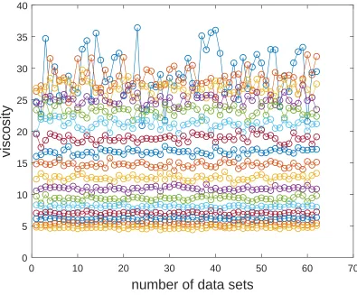
obtained from a single run. A run of 5_×105_{, 1.5×10}6_{, 2×10}6 _{time steps produces,}

respec-tively, 15, 46 and 62 data sets. For each data set, TCAFs are obtained by averaging 500

overlapping samples in which measurements are made every 5 time steps and there are 1025

measurements per sample. It is observed that using a larger number of data sets make the

solution behaviour with respect to the wave number more stable. In the following sections,

the obtained results from 62 data sets are presented. Both Newtonian and viscoelastic fitting

models are applied to the same TCAF data (i.e. C⊥(k, t)/C⊥(k,0)). Their resultant curve

fits are observed to be graphically the same; only those for the Newtonian case are displayed.

For a time step, the elapsed CPU time of computing TCAF is insignificant compared to that

of solving the DPD equations of motion.

6.1

Newtonian fluids

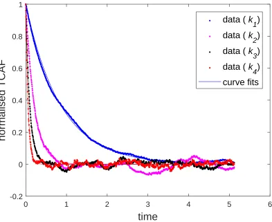
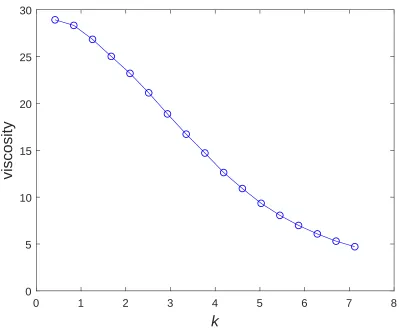
Some typical variations of TCAF are displayed in Figures 1. Since the finite size, defined

through wavelength, is taken into account, the Newtonian viscosity estimated from TCAF

is a function of the wave number. The obtained results are shown in Figures 2 and 3. One

has a wave number-dependent viscosity with the observation time scale being assumed to

be large. To obtain the viscosity at k = 0 (a continuum), some extrapolation is needed. As

whereη0 anda are two fitting parameters. Assuming that values ofk used for the fitting are

sufficiently small, η0 can be regarded as the viscosity at the hydrodynamic limit. Using the

first 4 smallest values ofk(i.e. 0.4189, 0.8378, 1.2566 and 1.6755), this leads toη0 = 29.0214.

On the other hand, from the kinetic theory [1], the viscosity is estimated as η = 30. The

advantage of the TCAF approach is that it can provide information about the size effect

on the transport properties. In addition, one can estimate the transport coefficients at the

hydrodynamic limit through extrapolation.

6.2

Linear viscoelastic fluids

6.2.1 Wavelength- and frequency-dependent transport coefficients

The stress approximations involve two parameters, the viscosity and relaxation time, which

are wavelength- and frequency-dependent.

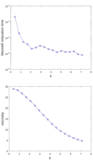
Figure 4 shows plots of the viscosity and the decay constant of the memory function against

the wave numberk. Whenk decreases, the decay constant τk is seen to increase quickly and

is expected to reach its maximum in the hydrodynamic limit. For the shear viscosity ηk, the

change is observed to be slow as k_→0. The obtained values of ηk here are similar to those

in the Newtonian case.

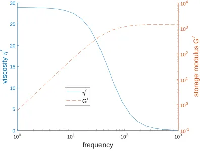
Figure 5 displays the storage modulus and viscosity against the frequency ω, according to

(42) and (43), for the first (smallest) value of k (i.e. k = k1 = 0.4189). At small values of

the frequency (i.e. large observation time scale), the system responses like a fluid and at

large values of the frequency, one has a solid-like response. The storage modulus provides a

convenient means of quantifying the level of elasticity of the fluid.

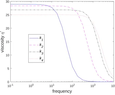
Figure 6 displays the shear viscosity against the frequency ω for the first four values of k

(i.e. 0.4189, 0.8378, 1.2566 and 1.6755). It can be seen that η′ _{→ η}

k as ω →0 and η′ → 0 as ω_{→ ∞}.

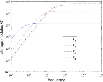
It can be seen that G′ _{→0 as ω→0 and G}′ _→η

k/τk as ω→ ∞.

6.2.2 Linear viscoelastic effect

As shown above, a DPD model using a single set of particles can result in a linear viscoelastic

fluid for k_≥0. A concern here is how to quantify the linear viscoelastic effect. Some typical

scenarios are studied below and some comments are given at the end of this section. Table

1 displays values of the original DPD parameters γ and s that correspond to the input

viscosities and Schmidt numbers imposed here.

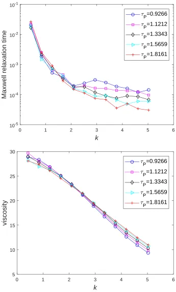
Same fluid at different imposed kBT

Five values of kBT, (1, 1.1, 1.2, 1.3, 1.4), are employed in conjunction with (ρ= 4, Sc = 500

and η= 30). They lead to τP = (0.93,1.12,1.33,1.57,1.82), respectively, according to (57).

The obtained results concerning the effects of the particle diffusion time τP on the relaxation

time of the memory kernel, τk, over a wide range of k are shown in Figure 8.

Fluids of different viscosities

Four values of η, (30, 28, 26, 24), are employed in conjunction with (ρ = 4, Sc = 500 and

kBT = 1). Figure 9 shows the effects of the imposed viscosity η on the relaxation time τk

over a wide range of k.

Fluids of different Schmidt numbers

Four values of Sc, (500, 600, 700, 800), are employed in conjunction with (ρ = 4, η = 30

and kBT = 1). Figure 10 shows the effects of the imposed limit Schmidt number Sc on the

relaxation time τk over a wide range of k.

From the three figures, it can be seen that the relaxation time, corresponding to different

values of τP, η or Sc, apparently converges as k is reduced, and one would expect that an

the particle diffusion time, viscosity or Schmidt number. An increase in τP, a decrease inη

or an increase in Sc results in a decrease in τk. Differences of τk at small k are thus much

smaller than those at large k. It can also been seen that a change in Sc orτP can affect the

estimated viscosity at the hydrodynamic limit.

7

Concluding remarks

In this work, DPD in its generalised hydrodynamic regime is considered. For a

Newto-nian fluid, the stresses are obtained through a large-time averaging process; they involve

one fitting parameter, namely the viscosity, which is wavelength-dependent. For a linear

viscoelastic fluids, the stresses involve two fitting parameters, namely the viscosity and the

relaxation time, which are wavelength- and frequency-dependent. The wavelength

depen-dency of the transport coefficients is obtained numerically while their frequency dependepen-dency

can be computed analytically, which allow the effects of the length and time scales introduced

by physical phenomena to be determined. The DPD input parameters can be determined

from the viscosity, mass density, Schmidt number and diffusion time. Numerical experiments

indicate that (i) a fluid modelled from a single set of particles may not be Newtonian, but

linear viscoelastic, and any time dependent effects must be carefully looked at, and (ii) the

relaxation time measuring the linear viscoelastic effect can be adjusted by means of the input

diffusion time, viscosity or Schmidt number at finite wave numbers.

References

1. Marsh C. Theoretical Aspects of Dissipative Particle Dynamics (D. Phil. Thesis).

University of Oxford; 1998.

2. Ripoll M, Ernst MH, Espa˜nol P. Large scale and mesoscopic hydrodynamics for

dissi-pative particle dynamics. J Chem Phys 2001;115(15):7271-7284.

4. Hansen JP, McDonald IR. Theory of Simple Liquids. 3rd ed. London: Academic Press;

2006.

5. Phan-Thien N, Mai-Duy N. Understanding Viscoelasticity: An Introduction to

Rheol-ogy. 3rd ed. Cham (Switzerland): Springer International Publishing; 2017.

6. Hess B. Determining the shear viscosity of model liquids from molecular dynamics

simulations. J Chem Phys 2002;116(1):209-217.

7. Vogelsang R, Hoheisel C. Computation and analysis of the transverse current

autocor-relation function, Ct(k,t), for small wave vectors: A molecular-dynamics study for a

Lennard-Jones fluid. Phys Rev A 1987;35(4):1786-1794.

8. Mai-Duy N, Phan-Thien N, Tran-Cong T. An improved dissipative particle dynamics

scheme. Appl Math Model 2017;46:602-617.

9. Mai-Duy N, Phan-Thien N, Tran-Cong T. Imposition of physical parameters in

dissi-pative particle dynamics. Comput Phys Comm 2017;221:290-298.

10. Groot RD, Warren PB, Dissipative particle dynamics: Bridging the gap between

atom-istic and mesoscopic simulation, J Chem Phys 1997;107:4423-4435.

11. Palmer BJ. Transverse-current autocorrelation-function calculations of the shear

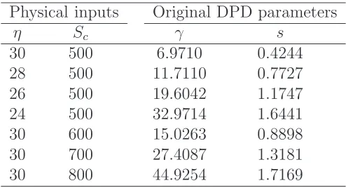
Table 1: Values of the input viscosity and Schmidt number, and the corresponding original DPD parameters for (m = 1, n = 4, kBT = 1, rc = 1.5).

Physical inputs Original DPD parameters

η Sc γ s

0 1 2 3 4 5 6

time

-0.2 0 0.2 0.4 0.6 0.8 1

normalised TCAF

data ( k

1

)

data ( k

2

)

data ( k

3

)

data ( k

4

)

curve fits

0 10 20 30 40 50 60 70

number of data sets

0 5 10 15 20 25 30 35 40

viscosity

0 1 2 3 4 5 6 7 8

k

0 5 10 15 20 25 30

viscosity

0 1 2 3 4 5 6 7 8

k

10-5

10-4

10-3

10-2

10-1

Maxwell relaxation time

0 1 2 3 4 5 6 7 8

k

0 5 10 15 20 25 30

viscosity

100 101 102 103

frequency

0 5 10 15 20 25 30

viscosity

10-1 100 101 102 103 104

storage modulus G

G

Figure 5: Viscoelastic fluids: Storage modulus and viscosity as functions of the frequency for the smallest wave number (i.e. k =k1 = 0.4189). The system responses like a fluid at small

10-1 100 101 102 103 104

frequency

0 5 10 15 20 25 30

viscosity

k

1

k

2

k

3

k

4

Figure 6: Viscoelastic fluids: Viscosity as a function of the frequency for the first four values of k (i.e. 0.4189, 0.8378, 1.2566 and 1.6755). It can be seen that η′ _{→ η}

101 102 103 104 105 106

frequency

10-1

100

101

102

103

104

105

storage modulus G

k

1

k

2

k

3

k

4

Figure 7: Viscoelastic fluids: Storage modulus as a function of the frequency for the first four values of k (i.e. 0.4189, 0.8378, 1.2566 and 1.6755). It can be seen that G′ _{→ 0}

as ω _→ 0 and G′ _{→ η}

0 1 2 3 4 5 6

k

10-5 10-4 10-3 10-2 10-1

Maxwell relaxation time

P=0.9266

P=1.1212

P=1.3343

P=1.5659

P=1.8161

0 1 2 3 4 5 6

k

5 10 15 20 25 30

viscosity

P=0.9266

P=1.1212

P=1.3343

P=1.5659

P=1.8161

0 1 2 3 4 5 6

k

10-6 10-5 10-4 10-3 10-2 10-1

Maxwell relaxation time

=30 =28 =26 =24

0 1 2 3 4 5 6

k

5 10 15 20 25 30

viscosity

=30 =28 =26 =24

0 1 2 3 4 5 6

k

10-6 10-5 10-4 10-3 10-2 10-1

Maxwell relaxation time

S

c=500

S

c=600

S

c=700

S

c=800

0 1 2 3 4 5 6

k

5 10 15 20 25 30

viscosity

S

c=500

S

c=600

S

c=700

S

c=800