A geometric study of commutator subgroups

A Geometric Study of Commutator Subgroups

Thesis by

Dongping Zhuang

In Partial Fulfillment of the Requirements for the Degree of

Doctor of Philosophy

California Institute of Technology Pasadena, California

2009

Acknowledgments

I am deeply indebted to my advisor Danny Calegari, whose guidance, stimulating suggestions and encour-agement help me during the time of research for and writing of this thesis.

Thanks to Danny Calegari, Michael Aschbacher, Tom Graber and Matthew Day for graciously agreeing to serve on my Thesis Advisory Committee.

Thanks to Koji Fujiwara, Jason Manning, Pierre Py and Matthew Day for inspiring discussions about the work contained in this thesis.

Thanks to my fellow graduate students. Special thanks to Joel Louwsma for helping improve the writing of this thesis.

Thanks to Nathan Dunfield, Daniel Groves, Mladen Bestvina, Kevin Wortman, Irine Peng, Francis Bonahon, Yi Ni and Jiajun Wang for illuminating mathematical conversations.

Thanks to the Caltech Mathematics Department for providing an excellent environment for research and study.

Thanks to the Department of Mathematical and Computing Sciences of Tokyo Institute of Technology; to Sadayoshi Kojima for hosting my stay in Japan; to Eiko Kin and Mitsuhiko Takasawa for many interesting mathematical discussions.

Abstract

LetGbe a group andG0 its commutator subgroup. Commutator length (cl) and stable commutator length (scl) are naturally defined concepts for elements ofG0. We study cl and scl for two classes of groups. First, we compute scl in generalized Thompson’s groups and their central extensions. As a consequence, we find examples of finitely presented groups in which scl takes irrational (in fact, transcendental) values. Second, we study large scale geometry of the Cayley graphCS(G0)of a commutator subgroupG0 with respect to

the canonical generating setS of all commutators. WhenGis a non-elementaryδ-hyperbolic group, we prove that there exists a quasi-isometrically embeddedZn_inC

S(G0), for eachn∈Z+. Thus this graph is

Contents

Acknowledgments iv

Abstract v

1 Introduction 1

2 Commutator Length 5

2.1 Definitions of Commutator Length . . . 5

2.2 Group Homology and Commutator Length . . . 6

2.3 Computations of Commutator Length . . . 8

3 Stable Commutator Length 11 3.1 Definitions of Stable Commutator Length . . . 11

3.2 Quasimorphisms and Bavard’s Duality Theorem . . . 13

3.2.1 Definition of Quasimorphisms . . . 13

3.2.2 Bounded Cohomology and Bavard’s Duality Theorem . . . 14

3.3 Further Properties and Constructions of Quasimorphisms . . . 17

3.3.1 Rotation Number . . . 17

3.3.2 Counting Quasimorphisms . . . 19

4 SCL in Generalized Thompson’s Groups 21 4.1 Thompson’s Groups and Generalized Thompson’s Groups . . . 21

4.2 Homology of Generalized Thompson’s Groups . . . 24

4.2.1 Construction ofX . . . 24

4.2.2 Costruction ofN . . . 26

4.2.3 Collapsing to a Complex of Finite Type . . . 30

4.2.4 More Collapsings and Construction of a CW-complex . . . 32

4.3 SCL in Generalized Thompson’s Groups . . . 36

4.3.1 Main Theorem . . . 36

5 Large Scale Geometry of Commutator Subgroups 45

5.1 Commutator Subgroup as a Metric Space . . . 45

5.2 Large Scale Geometry of Metric Spaces . . . 48

5.3 Large Scale Simple Connectivity . . . 52

5.4 Hyperbolicity and Large Scale Geometry . . . 56

5.4.1 Hyperbolic Groups . . . 57

5.4.2 Generalized Counting Quasimorphisms . . . 58

5.4.3 Quasi-isometrically EmbeddedZn . . . 59

5.4.4 Large Scale Connectivity at Infinity . . . 64

List of Figures

4.1 x0(left) andx1(right). . . 22

4.2 An expansion(a= 3, n1= 2). . . 25

4.3 A forest. . . 26

4.4 Elementary (left) and non-elementary (right) simplexes. . . 27

4.5 A triangulated3-cube. . . 27

4.6 A non-cubic structure. . . 28

4.7 Part of the maximal tree. . . 29

4.8 A relation from a2-cube. . . 29

4.9 A forest representingv2x1x1,2v(n1= 2andn2= 3). . . 30

4.10 The pushing defined byd2. . . 32

4.11 y0(left) andy+0 (right). . . 36

4.12 The homeomorphismg. . . . 37

4.13 Graph off. . . 41

4.14 Graph oft. . . . 42

4.15 Graph ofg. . . . 42

4.16 Graph ofh. . . . 43

5.1 A standard basis forπ1(Σ)whereΣhas genus4. Theαicurves are in red, and theβicurves are in blue. . . 53

Chapter 1

Introduction

LetGbe a group andG0 = [G, G]its commutator subgroup. Elements ofG0are products of commutators. The commutator length (denoted cl) of an elementg∈G0_{is defined to be the least number of commutators}

whose products equals g. The stable commutator length (denoted scl) of g is the stabilized commutator length, i.e., the limit of cl(gn_{)/n, asn → ∞. cl and scl have been studied not only in group theory, but}

also in topology, usually as genus norms. In the later case, there are two geometric approaches. The first is to use the topological definitions of cl and scl directly. In this approach, one essentially studies maps of surfaces (with boundaries) into spaces and tries to find the “simplest” one among them. The second approach comes from the deep connection of scl with bounded group cohomology. The main tool in this direction is the concept of (homogeneous) quasimorphisms. Quasimorphisms are homomorphisms up to bounded errors, and, surprisingly, many important invariants from geometry and dynamical systems can be regarded as quasimorphisms. The connection between scl and quasimorphisms comes from Bavard’s Duality Theorem, which states that the set of all homogeneous quasimorphisms determines scl. One can also obtain nontrivial estimates of cl from quasimorphisms.

The purpose of this paper is to study arithmetic and geometric properties of cl and scl. We adopt the second approach via quasimorphisms. We study two classes of finitely generated groups which have different spaces of homogeneous quasimorphisms. The first class of groups is generalized Thompson’s groups and their central extensions. Elements in these groups can be interpreted as automorphisms of the unit circle or the real line. We prove that the spaces of homogeneous quasimorphisms of these groups have finite dimensions (in fact0or1), and when the dimension is1, the only nontrivial (normalized) homogeneous quasimorphism is given by the rotation quasimorphism. Thus the computation of scl is reduced to that of rotation numbers. As a consequence, we have the following irrationality theorem:

Theorem A ([60]). There are finitely presented groups, in which scl takes irrational (in fact, transcendental)

values.

values. Calegari’s computation in free groups and Thurston’s norm in3-dimensional topology give important evidence of this. Our examples from generalized Thompson’s groups display a totally different phenomenon. The second class of groups are hyperbolic groups. In contrast to the first class of groups considered above, the spaces of homogeneous quasimorphisms of these groups are infinite dimensional, which has many geo-metric interpretations. One is through the notion of bounded cohomology, which says that the2nd bounded cohomology (withR-coefficients) of a hyperbolic group is infinite dimensional. In this paper, we give another interpretation through the large scale geometry of commutator subgroups. LetSbe the set of all commuta-tors, which form a canonical generating set forG0_{. LetC}

S(G0)be the Cayley graph ofG0with respect toS,

meaning the vertices ofCS(G0_{)are elements inG}0_{, and two elementsg}

1andg2are connected by an edge

ifg−₁1g2is inS. By identifying each edge with the unit interval (with length1),CS(G0)becomes a metric

space, on whichG0acts by isometries. Then cl is the path metric in this graph and scl equals the translation length of this action. Cayley graphs are the most studied objects in geometric group theory, and we are in-terested in the large scale geometry of these graphs, i.e., those properties invariant under quasi-isometries. Roughly speaking, under quasi-isometries, we throw away local structures and only focus on large scale (or long range) properties of metric spaces. In the case of the Cayley graph of a commutator subgroup, we prove that

Theorem B. LetGbe a non-elementary word-hyperbolic group andZn _{the integral lattice inR}n _{with the}

induced metric. Then, for anyn ∈ Z+, we have a mapρn:Zn → CS(G0), which is a quasi-isometric

embedding.

The proof implies that the geometry ofCS(G0)should be non-negatively curved and shows the existence of flats (zero curved subsets) of arbitrarily large dimensions. It uses counting quasimorphisms, constructed by R. Brooks [6] in free groups and Epstein-Fujiwara [27] in general hyperbolic groups. As a corollary of this theorem, we have

Corollary C. LetGbe a non-elementary word-hyperbolic group. Then we have 1. CS(G0)is notδ-hyperbolic;

2. asdim(CS(G0_{)) =∞;}

3. CS(G0)is one-ended, i.e.,CS(G0)is connected at infinity.

For a general group, we study the large scale topology of this graph and show that

Theorem D ([15]). LetGbe a finitely presented group. ThenCS(G0)is large scale simply connected.

Theorem B, Corollary C and Theorem D are joint work with D. Calegari.

Chapter 2

Commutator Length

In this chapter, we introduce the notion of commutator length. Commutator length is an algebraic invariant of elements in groups. It’s related to the topological concept of the genus of a surface . We are going to explore this connection through the theory of group (co)homology. At the end, we give examples, exemplifying the computations of commutator length in various groups, which are important in geometry and dynamical systems.

2.1

Definitions of Commutator Length

LetGbe a group. An elementa∈Gis a commutator if there existb, c∈G, such thata= [b, c] =bcb−1_c−1_.

LetG0 _{= [G, G]denote the normal subgroup of Gwhich is generated by commutators. We callG}0 _the

commutator subgroup ofGand they fit into a short exact sequence

1−→G0_{−→G−→G/G}0_−→0.

The quotient groupG/G0is, by its construction, the largest abelian quotient group ofGand whenGis finitely generated, this abelian quotient group is well understood by the classification theorem of finitely generated abelian groups. So in principle, to studyG, we only need to understand the commutator subgroupG0andG0 contains all the information lost in the quotient process. A natural measure of complexity for the elements in G0_{is the notion of commutator length.}

Definition 2.1.1. LetGbe a group anda∈G0. The commutator length ofa, denoted cl(a), is the smallest number of commutators whose product is equal toa, i.e.,

cl(a) = min{n|a= [b1, c1]· · ·[bn, cn], bi, ci∈G}.

Set cl(a) =∞if a is not an element inG0_.

(∗is the base point). An elementγ ∈ π1(X,∗)can be represented by a mapf: (S1,∗)→ (X,∗). Since

commutator length takes the same value in a conjugacy class, we only need to consider the conjugacy class ofγ, which can be interpreted as the free homotopy class of the mapf: S1_{→X. From now on, we sayγ}

is represented by a looplγ, the image of the mapf inX without the base point. Ifγis an element in the

commutator subgroupG0_{, we can write}

γ= [α1, β1][α2, β2]· · ·[αg, βg].

LetS be an oriented surface of genusgwith one boundary component. S is obtained from a(4g+ 1)-gon P by identifying edges in pairs and the edges ofPare labelled bya1b1a−11b−11· · ·agbga−g1b−g1c−1. Choose

the loops inX representingγ, αi, βi,1 ≤ i ≤ gand leth: ∂P → X be defined by sending edges ofP

to those loops inX byai → αi,bi →βiand the free edgectoγ. By the construction,hfactors through

the quotient map∂P → Sinduced by gluing up all but one of the edges. Moreover, by hypothesis,h(∂P)

represents[α1, β1]· · ·[αg, βg]γ−1= 1inπ1(X). Hencehcan be extended to a maph:S→X, sending∂S

toγ. Therefore a loop, corresponding to an element in[π1(X), π1(X)], bounds a map of an oriented surface

intoX and the number of commutators needed in the product is the genus of the surface. In this language, commutator length has the following equivalent definition

Definition 2.1.2. LetXbe a topological space andG=π1(X). Givenγ∈[π1(X), π1(X)], we have

cl(γ) = min

S∈Λ{genus(S)},

whereΛ ={h: S →X}andSis an oriented surface with one boundary component such thath(∂S)⊂γ and[h(∂S)] =±[γ]inH1(γ,Z).

If a loop γ bounds an oriented surface inX, then[γ], regarded as a dimension-1 homological class, represents the trivial element inH1(X) =π1(X)/[π1(X), π1(X)]. The commutator length ofγmeasures

the complexity of this triviality on the level of homology.

2.2

Group Homology and Commutator Length

In this section, we study the connection between commutator length and the theory of group (co)homology. The (co)homology theory of groups arose from both topological and algebraic sources. We briefly introduce the theory from both points of view and give a very rough interpretation of commutator length as a norm related to the homology of a group.

Definition 2.2.1. LetGbe a group. A CW-complexY is called an Eilenberg-Maclane complex of type(G,1) ifY satisfies the following conditions:

2. π1(Y)∼=G;

3. The universal coverYe ofY is contractible. Or equivalentlyHi(Ye) = 0fori≥2, orπi(Ye) = 0for i≥2.

By Hurewicz’s theorem, the homotopy type ofY is determined byG = π1(Y), and we denote it by

K(G,1). For any groupG, we can construct such a complex. Thus we have

Definition 2.2.2. LetGbe a group. The homology ofGwithZ-coefficients is defined to be the homology of the correspondingK(G,1), i.e.,

H∗(G,Z) =H∗(K(G,1),Z).

The homology of a group can also be defined using the bar complex.

Definition 2.2.3. LetGbe a group. The bar complexC∗(G)is the complex generated in dimensionnby n-tuples(g1, g2, . . . , gn)withgi∈G. The boundary map∂is defined by the formula

∂(g1, . . . , gn) = (g2, . . . , gn) +

n−1

X

i=1

(−1)i(g1, . . . , gigi+1, . . . , gn) + (−1)n(g1, . . . , gn−1).

With a coefficient groupR(=Z,Q,orR), define the homology of the groupGwith coefficients inRto beH∗(C∗(G)⊗R).

Alln-tuples(g1, g2, . . . , gn),gi ∈Gform a canonical basis for then-dimensional chain groupCn(G),

and we have the canonical inclusionsC∗(G,Z),→C∗(G,Q),→C∗(G,R). From now on, we’ll only useR

as the coefficient group, and the elements inC∗(G,Z)orC∗(G,Q)will be called integral or rational chains. Let[c]be a homology class inHi(G,R). We can writec = Priσi ∈ Ci(G,R), ri ∈ R, as a chain

representative of[c]. Define

kck1=

X

i

|ri|.

Definition 2.2.4. The (Gromov) L1-norm of[c]∈Hi(G)is defined by

k[c]k1= inf

c kck1,

wherecranges over all chain representatives of[c]inCi(G).

Denote the cycles and the boundaries withR-coefficients byZ∗(G)andB∗(G)respectively. Then we have, in dimension2, a short exact sequence

0−→Z2(G)−→i C2(G)−→∂ B1(G)−→0.

Definition 2.2.5. Leta∈B1(G). The (Gersten) boundary norm ofa, denotedkakB, is defined by

kakB= inf A∈C2(G),∂A=a

kAk1.

The groupGincludes as a canonical basis inC1(G). Ifais an element inG0, then the image of ain

C1(G)lies inB1(G). In fact,a∈G0implies thata, thought of as a loop, bounds an oriented surface with one

boundary component. A one-vertex triangulation of this surface, with the only vertex on the boundary, gives an expression ofaas an element inB1(G). For example, ifa= [x, y], we have∂((xyx−1, x) + ([x, y], y)−

(x, y)) = [x, y]. Recall the topological definition of commutator length, which gives an interpretation of cl as a measure of complexity among all the surfaces withaas the only boundary component. It’s not difficult to see, through counting the number of triangles, that ifa∈[G, G],

kakB≤4cl(a)−1.

It’s not clear whether there exists an inequality in the opposite direction. And one way to overcome this difficulty is to “stabilize” both the boundary norm and commutator length, which will give an equality between them. Roughly speaking, we need to identify g_nn andgfor anygand consider the boundary norm under this identification. In Chapter2, we will explore this idea and study stable commutator length.

2.3

Computations of Commutator Length

In this section, we do computations of commutator length. Some of the groups are the special examples of more general classes of groups we are going to study in the following chapters.

2.3.1 Commutator length in free groups. Commutator length in free groups has been studied by many people. C. C. Edmunds in [22] [23] first showed that there exists an effective procedure for comput-ing commutator length in free groups. M. Culler, uscomput-ing surface theory, also worked out an algorithm for computing commutator length, which we will describe below. See [17] for more details.

LetTnbe an orientable surface of genusnwith one boundary component. LetΓrbe the wedge product

ofrcircles, then the fundamental group ofΓris free onrgenerators. So questions about commutator length in a free group translate into questions about maps fromTntoΓr. M. Culler shows that ifw∈[Fr, Fr]has

commutator lengthnandf: Tn →Γris any map such thatf(∂Tn)representsw, thenf is homotopic to a

“tight” map. Supposewis written as a reduced word, then each “tight” map gives a “pairing” of the letters in w. Conversely, given a “pairing” of the letters inw, we can construct a unique (up to homotopy) “tight” map and the genus of the surface can be read from the combinatorial information of the “pairing”.

1. Ifa1, b1,· · ·, an, bnare elements of a basis of a free group, then we have

cl([a1, b1]· · ·[an, bn]) =n.

2. Ifa, bare basis elements in a free group, then

cl([a, b]n) =bn

2c+ 1.

And we also obtain interesting commutator identities, for example

[a, b]3_{= [aba}−1_{, b}−1_aba−2_][b−1_{ab, b}2_].

2.3.2 Commutator length in Homeo+(S1_{). Let Homeo}+_(S1_{)be the group of orientation-preserving}

homeomorphisms of the circle. Every element in Homeo+(S1_{)can be written as a product of two elements}

both of which have a fixed point. And a homeomorphism in Homeo+(S1_{)with a fixed point can be written as}

a commutator. (In fact, such an element is conjugate to its square.) So cl≤2in Homeo+(S1). Furthermore, one can show that cl≤1in Homeo+(S1). See [25] for more details.

2.3.3 Knots in3-sphere. A knotγis an embedding: γ: S1 →S3. A Seifert surface for a knotγis a connected, two-sided, compact embedded surfaceΣ ⊆S3 with∂Σ = γ. Define the genus of a knotγ, denotedg(γ), to be the least genus of all its Seifert surfaces. It follows from a deep theorem of D. Gabai [33] thatg(γ) =cl(γ), whereγis regarded as an element inπ1(S3\N(γ))andN(γ)is an open neighborhood of

γ. Genus of a knot is a very important knot invariant.

2.3.4 Commutator length in mapping class groups. Mapping class group is a fundamental object in2-dimensional topology. See [4] and [28] for more details.

Definition 2.3.2. LetSbe an oriented surface (possibly punctured). The mapping class group ofS, denoted MCG(S), is the group of isotopy classes of orientation-preserving self-homeomorphisms ofS.

MCG(S)is finitely presentable and its generating set can be chosen from a special class of elements, called Dehn twists.

Definition 2.3.3. Letγ be an essential simple closed curve inS. A right-handed Dehn twist inγ is the maptγ:S →Ssupported on an annulus neighborhoodγ×[0,1]which takes each curveγ×tto itself by

a positive twist through a fractiont of its length. If the annulus is parameterized asR/Z×[0,1], then in coordinates, the map is given by(θ, t)→(θ+t, t).

Theorem 2.3.4 ([47]). Leta∈MCG(S)be a Dehn twist in a nonseparating closed curve. Thena10_{can be}

Chapter 3

Stable Commutator Length

In this chapter, we continue the study of group (co)homology and define stable commutator length both al-gebraically and topogically. A very important tool in the study of stable commutator length is the notion of (homogeneous) quasimorphisms. We sketch the proof of Bavard’s theorem (3.2.10), which shows the duality between stable commutator length and homogeneous quasimorphisms. At the end, we give the explicit con-structions of quasimorphisms in Homeo+(S1)and free groups. These quasimorphisms will play important roles in the next two chapters.

3.1

Definitions of Stable Commutator Length

Definition 3.1.1. LetGbe a group anda ∈G. The stable commutator length ofa, denoted scl(a), is the following limit

scl(a) = lim

n→∞

cl(an) n . Set scl(a) =∞, if no power ofais in[G, G].

Commutator length cl clearly has the subadditive property, i.e., cl(am+n_)≤cl(am_{) +cl(a}n_{). Then the}

existence of the limit in the definition follows from the lemma below.

Lemma 3.1.2. Ifam+n≤am+an+L, for allm, n∈Nand some fixedL, thenlimn→∞an/n∈R∪{−∞}

exists.

Proof. Suppose

lim inf n→∞

an

n < b < c, then there existsn,n > 2L

c−b such that an

n < b. For sufficiently largel,l > n,l(c−b)>2 maxr<nan, write

l=nk+r,0< r < n, and al

l ≤

kan+ar+kL

l ≤ an n + ar l + L n ≤b+

c−b

2 +

c−b

Thuslim supn→∞an/n= lim infn→∞an/n, and the limit exists.

Remark 3.1.3. cl and scl are invariant under the action of Aut(G), where Aut(G)is the group of automor-phisms ofG. In particular, they are conjugacy invariant.

Stable commutator length also has a topological description. Let G ∼= π1(X)andγ is a loop in X,

representing the conjugacy class of an elementa ∈ G. One easily sees, from the topological definition of cl, that scl(a)equals the infimum of genus(S)/n(S), whereSis a connected, oriented surface with only one boundary component andS admits a map intoX with∂Swrapping aroundγ n(S)times. One deficiency of this definition is that this infimum will never be achieved. For any such surface S with one boundary component, we can pass to finite covers ofSand genus(S)/n(S)can be reduced to −χ_2n((_SS₎), whereχ(S)is the Euler characteristic ofS. Therefore we have the following alternative topological definition for stable commutator length.

Let G, X, a, γ be as above. Given a compact, oriented, not necessarily connected surface S, define −χ−_{(S)to be the sum ofmax(−χ,0)over all components ofS. Given a mapf:S →X, taking∂S→γ,}

definen(s)to be the sum, over all components of∂S, of the degree of the mapf|∂S, i.e.,f∗[∂S] =n(S)[γ],

where[γ]is the generator ofH1(γ,Z).

Proposition and Definition 3.1.4 ([9]). LetG=π1(X)andγ⊂Xa loop representing the conjugacy class

ofa∈G. Then

scl(a) = inf S

−χ−_(S) 2n(S) ,

where the infimum is taken over all mapsf: (S, ∂S)→(X, γ).

Definition 3.1.5. A surfaceS, admitting a mapf: (S, ∂S)→(X, γ)which realizes the infimum of −χ_2n−_(S(S₎), is said to be extremal.

Example 3.1.6.

1. Ifa, bare basis elements in a free group, by Example (2.3.1), we have

scl([a, b]) = lim

n→∞

bn

2c+ 1

n =

1 2.

2. In Homeo+(S1_{), cl is bounded (≤1). So by definition, scl≡0.}

3. In mapping class groups, interesting lower bounds of scl can be obtained using gauge theory.

Theorem 3.1.7 (Endo-Kotschick [26], Kotschick [48]). LetSbe a closed orientable surface of genus g ≥2. Ifa∈ MCG(S)is the product ofkright-handed Dehn twists along essential disjoint simple closed curvesγ1,· · · , γk, then

scl(a)≥ k

Theorem 3.1.8 (Kotschick). Iftis a Dehn twist along a non-separating curve in a closed orientable surface of genusg, there is an estimate scl(t) =O(1

g).

3.2

Quasimorphisms and Bavard’s Duality Theorem

In this section, we introduce the notion of quasimorphisms. Quasimorphisms are related to our study of stable commutator length by Bavard’s duality theorem. In fact the content of this paper is the application of quasimorphisms and Bavard’s theorem to the study of commutator subgroups, and this section is the foundation of the whole paper.

3.2.1

Definition of Quasimorphisms

Definition 3.2.1. LetGbe a group. A quasimorphism onGis a function

φ:G→R,

for which there is a constantD(φ)≥0such that for anya, b∈G, we have an inequality

|φ(a) +φ(b)−φ(ab)| ≤D(φ).

In other words, a quasimorphism is like a homomorphism up to a bounded error. The least constantD(φ) with this property is called the defect ofφ.

Definition 3.2.2. A quasimorphism is homogeneous if it satisfies the additional property

φ(an) =nφ(a)

for alla∈Gandn∈Z.

Remark 3.2.3. D(φ) = 0if and only ifφis a homomorphism, i.e.,φ∈Hom(G,R). And it’s not difficult to see that a homogeneous quasimorphism is a class function.

Denote the sets of quasimorphisms and homogeneous quasimorphisms byQb(G)andQ(G)respectively. Givenφ∈Qb(G), we can homogenize it to obtain a homogeneous quasimorphism.

Lemma 3.2.4 ([9]). φ∈Qb(G)withD(φ). Then for anya∈G, the limit

φ(a) = lim n→∞

φ(an₎

n

3.2.2

Bounded Cohomology and Bavard’s Duality Theorem

We defined bar complex C∗(G,R)and used it to define the homology of a group G. Let C∗(G,R) = Hom(C∗(G),R)be the dual chain complex andδthe adjoint of∂. The homology group of(C∗(G,R), δ)is called the cohomology group ofGwith coefficients inRand is denotedH∗(G,R).

The chain groupC∗(G)has a canonical basis, consisting of alln-tuples(g1,· · ·, gn),gi∈G, in

dimen-sionn. A cochainα∈Cn_{(G,R)is called bounded if}

sup|α(g1,· · ·, gn)|<∞,

where the supremum is taken over alln-tuples. This supremum is called the L∞-norm ofα, and is denoted k αk∞. The set of all bounded cochains forms a subcomplexCb∗(G,R)and its homology is the so-called

bounded cohomology ofGand is denotedH∗

b(G). k · k∞ induces a (pseudo)norm onHb∗(G)defined as

follows: if[α]∈H∗

b(G)is a bounded cohomology class, setk [α]k∞= inf kσk∞, where the infimum is

taken over all bounded cocyclesσin the class of[α].

Let’s see what these definitions mean in low dimensions. A dimension-1cochainφ ∈ C1(G)is just a real-valued function fromGtoRandφis a cocycle if and only ifδφ= 0. By the definition of the coboundary map,

δφ(a, b) =φ(a) +φ(b)−φ(ab).

Thusφis a cocycle if and only ifφis a homomorphism andH1(G,R)can be identified with Hom(G,R). Since any nontrivial homomorphism fromGtoRis unbounded, it’s immediate thatH_b1(G,R) = 0for any groupG.

Supposeφis a quasimorphism defined above, then

|δφ(a, b)|=|φ(a) +φ(b)−φ(ab)| ≤D(φ),

for anya, b∈G. Thusδφis by definition a bounded2-cochain, i.e.,δφ∈C_b2(G,R)andkδφk∞=D(φ). Since δφis obviously a cocycle, we get that the image of the coboundary map of a quasimorphism is a bounded dimension-2cocycle. Furthermore, we have

Theorem 3.2.5 ([9]). There is an exact sequence

0−→H1_{(G,R)−→Q(G)} δ

−→H2

b(G,R)→H2(G,R).

Proof. Consider the short exact sequence of cochain complexes

and the associated long exact sequence of cohomology groups. We get an exact sequence

0 =H1

b(G,R)−→H1(G,R)−→H1(C∗/Cb∗)−→Hb2(G,R)−→H2(G,R).

AndH1_(C∗_/C∗

b) =Q/Cb b1∼=Q. We are done.

Recall that in Chapter1, we defined (Gersten) boundary normk · kB on B1(G,R), the dimension-1

boundary group and we tried to explore the relation betweenkakBand cl(a)for an elementa∈[G, G]⊂

B1(G,R). In the following, we stabilize both of the notions and obtain an equality between them.

Proposition 3.2.6 ([9]). Leta∈[G, G], so thata∈B1(G)as a cycle. Then

kakB= sup φ∈Qb(G)/H1_(G,R)

|φ(a)| D(φ).

Proof. The dual space ofB1(G)with respect to thek · kB norm isQb(G)/H1(G,R)and the operator norm

on the dual is equal toD(·) =kδ· k∞. Then the equality follows from Hahn-Banach Theorem.

Definition 3.2.7. LetG, abe as above. Define the filling norm, denoted fill(a), to be the homogenization of kak∞. That is

fill(a) = lim n→∞

kan_k B

n . Remark 3.2.8. fill(a)is the stabilized (Gersten) bounded norm.

Proposition 3.2.9 ([9]). LetGbe a group anda∈G0_{. There is an equality}

scl(a) =1 4fill(a).

Proof. We have known that for an elementa∈[G, G]and anyn∈Z+_,

kan_k

B≤4·cl(an)−1.

Divide both sides byn, take the limit asn→ ∞, and we get the inequality

fill(a)≤4·scl(a).

Conversely, assumeG=π1(X)andγis a loop inX, representing the conjugacy class ofa. letAbe a chain

with∂A=aandkAk1is close tokakB. WLOG, we assume thatAis a rational chain. After scaling by

some integer, we can assume thatAis an integral chain and∂A=nafor which the ratiokAk1/nkakB

is very close to1. WriteA =P_iniσi, where eachni ∈Z, and eachσi is a singular2-simplex, i.e., a map

gives us an orientable surfaceSand a mapΦ :S→X, such thatΦ∗([S, ∂S]) =A, where[S, ∂S]is a chain representing the fundamental class of(S, ∂S). By the construction,kAk1=k[S, ∂S]k1. About the Gromov

L1-norm of a surface, we have the following inequality

k[S, ∂S]k1≥ −2χ(S).

Dividing both sides byn, we get

fill(a)≥4·scl(a). Putting this with the earlier inequality, we are done.

Now combine Proposition (3.2.6) and Proposition (3.2.9) together, we get (see [1] or [9] for a proof) Theorem 3.2.10 (Bavard’s Duality Theorem [1]). LetGbe a group. Then for anya∈[G, G], we have an equality

scl(a) = 1

2φ∈Q(Gsup)/H1_(G,R)

|φ(a)| D(φ).

Remark 3.2.11.

1. Bavard’s theorem reflects the duality between scl and homogeneous quasimorphisms and the duality (i.e., Hahn-Banach theorem) is contained in Proposition (3.2.6).

2. In principle, given a groupG, we only need to work out the set of homogeneous quasimorphisms, and then we can compute scl by Bavard’s theorem. This approach is especially fruitful whenQ(G)has small dimension. In Chapter3, we are going to study several classes of finitely presented groups, of which the sets of homogeneous quasimorphisms are 1-dimensional.

3. There are many groups of which the sets of homogeneous quasimorphisms are infinite dimensional. In Chapter4, we will see that this is a common phenomenon in the groups related to hyperbolic geometry. Example 3.2.12. LetGbe a group. Recall that a mean onGis a linear functional onL∞_{(G)which maps the}

constant functionf(g)≡1to1, and maps non-negative functions to non-negative numbers.

Definition 3.2.13. A groupGis amenable if there is aG-invariant meanπ:L∞(G)→RwhereGacts on L∞_{(G)byg·f(h) =f(g}−1_{h), for allg, h∈Gandf ∈L}∞_(G).

Examples of amenable groups are finite groups, solvable groups (including abelian groups), and Grig-orchuk’s groups of intermediate growth.

Theorem 3.2.14 (Johnson, Trauber, Gromov). IfGis amenable, thenH_b∗(G,R) = 0. As a corollary of Theorem (3.2.5) and the theorem above, we have

3.3

Further Properties and Constructions of Quasimorphisms

The importance of quasimorphisms has been displayed by Bavard’s duality theorem (3.2.10). And in general, homogeneous quasimorphisms are easier to work with than ordinary quasimorphisms, but ordinary quasi-morphisms are easier to construct. They are related by the homogenization procedure (Lemma 3.2.4). In this section, we describe some important constructions of quasimorphisms in two classes of groups. Before that, we first mention a lemma about defect estimation. Supposeφis a homogeneous quasimorphism, then for any commutator[a, b]∈G, we have an inequality

|φ([a, b])| ≤D(φ).

And the following lemma says that this inequality is always sharp.

Lemma 3.3.1 (Bavard [1]). Letφbe a homogeneous quasimorphism onG. Then there is an equality

sup a,b∈G

|φ([a, b])|=D(φ).

3.3.1

Rotation Number

LetS1 _{= [0,1]/{0,1}be the unit circle andπ: R→S}1_{the covering projection. Let Homeo}+_(S1_{)be the}

group of orientation-preserving homeomorphisms ofS1_{. DefineHomeo}^+_(S1_{) ={f ∈Homeo}+_(R)|f(x+

1) = f(x) + 1}. It’s the subgroup of Homeo+(R), consisting of all the possible lifts of elements in Homeo+(S1_{)under the covering projectionπ.We have the central extension}

0−→Z−→Homeo^+(S1)−→p Homeo+(S1)−→1,

whereZis generated by the unit translation andp: Homeo^+(S1)→Homeo+(S1)is the natural projection. Definition 3.3.2. Forg∈Homeo^+(S1_{), define the rotation number ofg, denoted rot(g), to be}

rot(g) = lim

n→∞

gn₍₀₎

n .

Remark 3.3.3. Usually, rotation number is defined for elements in Homeo+(S1). Forf ∈ Homeo+(S1), choose an arbitrary liftf˜∈Homeo^+(S1)and the usual rotation number off is rot( ˜f) (modZ), which is a value inR/Z.

Rotation number is a very important dynamical invariant in Homeo+(S1_{). We put together some}

well-known properties of rotation number in the following proposition. ( See [45] for further discussions. ) Proposition 3.3.4.

2. rot(g)∈Qif and only ifp(g)∈Homeo+(S1_{)has a periodic point.}

3. If rot(g)is irrational andp(g)∈ Homeo+(S1)acts transitively onS1, thenp(g)is conjugate to the rotation through the angle rot(g)(modZ).

The following proposition shows that rotation number, as a function onHomeo^+(S1_{), is a homogeneous}

quasimorphism.

Proposition 3.3.5 ([60]). rot:Homeo^+(S1)→Ris a homogeneous quasimorphism and its defectD(rot) =

1.

Proof. First letf, g ∈ Homeo^+(S1). Without loss of generality, we assume that0 ≤ f(0), g(0) <1. So

0 ≤ f ◦g(0) < 2. And 0 ≤ rot(f) ≤ 1,0 ≤ rot(g) ≤ 1, and0 ≤ rot(f ◦g) ≤ 2. Thus we have |rot(f ◦g)−rot(f)−rot(g)| ≤ 2, and rot is a quasimorphism. rot being homogeneous is clear from its definition.

Second we show thatD(rot) = 1by using Lemma 3.3.1. Take anyf, g ∈ Homeo^+(S1). We want to compute rot([f, g]). We can still assume that0 ≤f(0), g(0)<1. Suppose0 ≤g(0)≤f(0)<1, then we have, by the fact thatf, gare both increasing functions:

g(f(0))< g(1) =g(0) + 1≤f(0) + 1≤f(g(0)) + 1.

So

f(g(0))−g(f(0))>−1

We have two cases:

(i) If we also havef(g(0))−g(f(0))≤1, then

−1≤f(g(0))−g(f(0))≤1,

g(f(−1)) =g(f(0))−1≤f(g(0))≤g(f(0)) + 1 =g(f(1)),

which implies

−1≤f−1_g−1_{f g(0)≤1 =⇒ |rot([f, g])| ≤1.}

(ii) If instead we havef(g(0))> g(f(0)) + 1, then

ConsiderH(x) =f−1_g−1_{f g(x)−1−x, forx∈[0,1].H(0) =f}−1_g−1_{f g(0)−1>0by assumption.}

H(f(0)) = f−1_g−1_{f g(f(0))−1−f(0)}

< f−1g−1f(f(0))−1−f(0) = f−1_g−1_f2_{(0)−1−f(0).}

We want to show thatH(f(0))<0, which can be deduced from the inequality below

f−1_g−1_f2_{(0)<1 +f(0),}

which is equivalent to

f2_{(0)< g(f}2_{(0)) + 1.}

This is always true sincex < g(x) + 1, for anyx∈R.

So we haveH(0)>0andH(f(0))<0, here0< f(0)<1. There must be a pointy∈(0, f(0))such that

H(y) =f−1_g−1_{f g(y)−1−y= 0.}

That is

f−1g−1f g(y) = 1 +y.

So

rot[f, g] = lim n→∞

[f, g]n_(y)−y

n = 1.

The proof for the case0≤f(0)≤g(0)<1is the same. Put all together, and we getD(rot) = 1.

3.3.2

Counting Quasimorphisms

Counting quasimorphisms were introduced by R. Brooks [6] in the study of bounded cohomology of free groups. Later on, this construction was generalized to word-hyperbolic groups by Epstein-Fujiwara [27] and more general classes of groups by Fujiwara [30] [31] and Bestvina-Fujiwara [2]. An immediate result of these constructions is that the 2nd bounded cohomology of these groups are infinite dimensional. In this section, we focus on free groups and give Brooks’ construction.

LetF be a free group with a finite free generating setS. Then any element inF has a unique reduced form, written as a word inS∪S−1_{. Letwbe a reduced word andg ∈F. The big counting functionCw(g)}

is defined by

and the little counting functioncw(g)is defined by

cw(g) =maximal number of disjoint copies ofwin the reduced representative ofg.

Definition 3.3.6. A big counting quasimorphism is a function of the form

Hw(g) =Cw(g)−Cw−1(g).

And a little counting quasimorphism is a function of the form

hw(g) =cw(g)−cw−1(g).

Example 3.3.7. LetF =F2=ha, bi.

1. Letw =aorb. It’s clear thatHw =hwin this case and they are both homomorphisms. In fact they

are the only cases in whichHworhwcould be a homomorphism.

2. Letw=aba, thenHw(ababa) = 2, buthw(ababa) = 1.

It’s not difficult to see that bothHw(·)andhw(·)are quasimorphisms with defects≤O(|w|), where|w| is the word length ofw. It turns out that for a big quasimorphismHw(·), its defectD(Hw)depends on|w|, but for a little quasimorphismhw(·), we have the following uniform bound for allw∈F.

Theorem 3.3.8 (D. Calegari [9]). LetF be a free group andw∈Fa reduced word. Lethw(·)be the little counting quasimorphism. Then we haveD(hw)≤2. More precisely, we have

1. D(hw) = 0if and only if|w|= 1;

2. D(hw) = 2if and only ifwis of the formw=w1w2w1−1,w=w1w2w−11w3orw=w1w2w3w−21as

reduced expressions;

3. D(hw) = 1otherwise. Remark 3.3.9.

1. The proof involves a careful analysis of the appearance ofworw−1in the junction where2reduced words are concatenated.

2. We know from the discussion before Theorem (3.2.5) that[δhw] ∈Hb2(F,R). A careful choice of a

sequence ofwi’s with|wi| → ∞will givehw’s such that the cohomology class[δhwi]’s are linearly

independent, implying that dimRHb2(F,R) =∞.

Chapter 4

SCL in Generalized Thompson’s Groups

In this chapter, we study scl in generalized Thompson’s groups. Generalized Thompson’s groups are very important objects in many branches of mathematics. They can be realized as subgroups of Homeo+(S1), and show a lot of interesting properties, similar to those of Homeo+(S1_{). For several classes of generalized}

Thompson’s groups, we prove that

1. For any groupT in these classes, the space of homogeneous quasimorphismsQ(T) = {0}. As a consequence,Q(Te)has dimension1and is generated by the rotation quasimorphism. HereTeis the central extension ofTbyZ.

2. Thus by Bavard’s Duality Theorem, we can compute scl inTe, and there are elements inT, whose scl’se take irrational (in fact, transcendental) values.

In contrast to bulletin2above, D. Calegari studies scl in free groups [12] (more generally, free product of abelian groups [13]) and shows that scl takes only rational values in them. And in general geometric settings, (relative) genus norms are expected to take rational values, like Thurston’s norm in3-dimensional topology. M. Gromov (in [36]6.C2) asked the question of whether such a stable norm, or in our content, the stable

commutator length in a finitely presented group, is always rational, or more generally, algebraic. And our computations give the negative answer.

4.1

Thompson’s Groups and Generalized Thompson’s Groups

LetFbe the set of piecewise linear homeomorphisms from the closed unit interval[0,1]to itself that are differentiable except at finitely many dyadic rational numbers (i.e., numbers of the formp·2q_{, p, q ∈Z) and}

such that on intervals of differentiability, the derivatives (slopes) are powers of2(i.e., numbers of the form

2m_{, m∈Z). It’s easy to verify thatFis a group and is called Thompson’s groupF.}

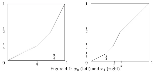
Example 4.1.1. Two elementsx0andx1inF, which are generators ofF.

1 4 1 2 1 0 1 2 3 4 1 0 1 8 1 4 1 2 1 4 3 8 1 2 1 1

Figure 4.1:x0(left) andx1(right).

The main properties ofF are contained in the following theorem. See [16] for proofs and further refer-ences.

Theorem 4.1.2.

1. Fis finitely presented and in fact FP∞, i.e., there is an Eilenberg-Maclane complexK(F,1)with finite

number of cells in each dimension.

2. The commutator subgroup[F, F]ofFconsists of all elements that are trivial in the neighborhoods of

0and1, i.e.,[F, F] =kerρ, whereρis the following homomorphism

ρ: F−→Z⊕Z

f 7−→(log2f0(0+),log2f0(1−)).

ThusF/[F, F]∼=Z⊕Z. 3. [F, F]is a simple group.

Next we define Thompson’s groupT. ConsiderS1_{as the unit interval[0,1]with the endpoints identified.}

ThenT is the set of piecewise linear homeomorphisms fromS1 = [0,1]/{0,1}to itself that map dyadic rational numbers to dyadic rational numbers and that are differentiable except at finitely many dyadic rational numbers and on intervals of differentiability, the derivatives (slopes) are powers of2.T is a group and called Thompson’s groupT.

There are several ways to generalize the definitions of Thompson’s groups. The one we are going to study is due to M. Stein [58]. LetP be a multiplicative subgroup of the positive real numbers and letAbe aZP-submodule of the reals withP A =A. Choose a numberl ∈A, l > 0. LetF(l, A, P)be the group of piecewise linear homeomorphisms of[0, l]with finitely many break points, all inA, having slopes only inP. Similarly defineT(l, A, P)to be the group of piecewise linear homeomorphisms of[0, l]/{0, l}(the circle formed by identifying endpoints of the closed interval[0, l]) with finitely many break points inAand slopes inP, with the additional requirement that the homeomorphisms sendA∩[0, l]to itself. It’s clear that F(l, A, P)⊂T(l, A, P). If we letP=h2iandA=Z[1₂], Thompson’s groups areF =F(1,Z[1₂],h2i)and T =T(1,Z[1

2],h2i).

We are interested in the case that P is generated by integers, i.e.,P = hn1, n2, . . . , nki and A =

Z[ 1

n1,

1

n2, . . . ,

1

nk]. P is a free abelian group and we can assume that {n1, n2, . . . , nk}forms a basis for

P, i.e.,logn1, . . . ,lognk areQ-independent, andkis the rank ofP. Let d = gcd(n1−1, . . . , nk −1)

andIP ·Athe submodule ofAgenerated by elements of the form(1−p)a, wherea∈Aandp∈P. An important theorem in studying generalized Thompson’s groups is the following Bieri-Strebel criterion. Theorem 4.1.4 (R. Bieri and R. Strebel [3]). Leta, c, a0, c0be elements ofAwitha < canda0< c0. Then there existsf, a piecewise linear homeomorphism ofR, with slopes inPand finitely many break points, all inA, mapping[a, c]onto[a0_{, c}0_{]if and only ifc}0_−a0_{is congruent toc−amoduloIP·A.}

Proof. Assume first that such anf exists. Leta = b0, b1, . . . , bn−1, bn = cbe an increasing sequence of

elements ofAsuch thatf is linear on[bi−1, bi]with slopepi, for alli. Thenc0−a0 =

Pn

i=1pi(bi−bi−1).

Butc−a=Pn_i=1(bi−bi−1), so(c0−a0)−(c−a)∈IP·A.

Conversely, suppose there exista1, . . . , an∈Aandp1, . . . , pn∈P such that

(c0−a0) = (c−a) + n

X

i=1

(1−pi)ai.

Setb0 _=c0_−a0_{andb=c−a. If we could findfmapping[0, b]to[0, b}0_{], composingfwith translation by}

−con the right andc0 _{on the left gives the desired map. Now there exists a permutationπof{1,2, . . . , n}}

such that the partial sumbj=b+

Pj

i=1(1−pπ(i))aπ(i)are positive forj = 0,1,2, . . . , n. Iff1, f2, . . . , fn

are piecewise linear homeomorphisms ofRwith slopes inP and break points inAsuch thatfi([0, bj−1]) =

[0, bj], thenfn◦ · · · ◦f1is the desiredf. Therefore it is sufficient to prove the claim forn= 1. Moreover,

as(1−p1)a= (1−p−11)(−p1a), we may assume thatp1>1. So we need to constructfmapping[0, b]to

[0, b+ (p−1)a], wherep >1,a= 06 (ifa= 0, the identity works), andbandb+ (p−1)aare both positive. Suppose first thata >0. Choose a numberkwitha < pkb, and seta0 =p−ka. Definef1, f2:R→Rby

f1(t) =

        

t ift≤b−a0,

p(t−(b−a0_{)) + (b−a}0_{) ifb−a}0_{< t≤b,}

f2(t) =

    

   

t ift≤b,

pk_{(t−b) +b ifb < t≤b+ (p−1)a}0_,

t+ (p−1)(a−a0_{) ifb+ (p−1)a}0 _{< t.}

Thenf1maps[0, b]to[0, b+ (p−1)a0]andf2maps[0, b+ (p−1)a0]to[0, b+ (p−1)a], sof =f2◦f1is

the desired map.

On the other hand, ifa <0then there existsftaking[0, b+ (p−1)a]to[0, b+ (p−1)a+ (p−1)(−a)] =

[0, b], sof−1will be the map we needed.

Remark 4.1.5. Ifd = gcd(n1−1, . . . , nk −1) = 1,IP ·A = P(dZ) = PZ = A, and the conclusion

in Theorem (4.1.4) is vacuously satisfied. Therefore in this case, we have that for anya < c, a0 _{< c}0_,

a, c, a0_{, c}0 _{∈A, there always exists anf with slopes inP and break points inA, such thatf maps[a, c]to} [a0_{, c}0_].

Theorem 4.1.6 (G. Higman [42]). LetΩbe a totally ordered set and letBbe a two-fold transitive, ordered permutation group onΩ, consisting of bounded elements. Then[B, B]is a nontrivial simple group.

Here “two-fold transitive” means that ifa < c,a0 < c0,a, c, a0, c0 ∈ Ω, then there is an element ofB takingatoa0 _andctoc0_{. LetΩ = IP ·A∩[0, l], then Theorem (4.1.4) tells us thatF(l, A, P)is two-fold}

transitive onΩ, so we have

Corollary 4.1.7. For any choice ofP,Aandl,F =F(l, A, P)has a simple commutator subgroup.

M. Stein also proves similar simplicity result for the groupT.

Theorem 4.1.8 ([58]). For any choice ofP,Aandl,T(l, A, P)has a simple second commutator subgroup.

4.2

Homology of Generalized Thompson’s Groups

To study scl on generalized Thompson’s groups, we need to know the perfectness of some subgroups of F = F(l, A, P), which can be deduced from the information on the dimension-1 homology group of F. M. Stein constructs a contractible CW-complex K, on whichF acts freely. So K/F is a K(F,1) and H∗(F,Z) ∼= H∗(K/F,Z). In the following, we give details of this construction, from which the desired property ofH1(F)easily follows. Most of the materials in this section are taken from M. Stein’s paper [58].

4.2.1

Construction of

X

TheX was first constructed by K. S. Brown [7], and Brown used it to show thatF =F(l, A, P)is finitely presented and of typeF P∞. Its costruction comes from a poset on which the groupF acts. Let’s describe

From now on, we’ll fixP =hn1, n2, . . . , nki,A=Z[_n1₁,_n1₂, . . . ,_n1_k], whereni’s∈Z+form a basis for

Pandl∈Z+_{∩A. An element of the poset is a piecewise linear homeomorphism from[0, a]to[0, l], where}

a∈Z,a≡l(modd), which has finitely many break points, all inA, and slopes inP. The “modd” condition comes from Theorem (4.1.4), by which such a homeomorphism exists if and only ifa−l ∈ IP ·A. And A/IP·A∼=Z/dZ, thus we can have such a map if and only ifa−l≡0(modd). Givenf1: [0, a]→[0, l],

we say f2 is a simple expansion of f1 if for somei, there exists s: [0, a+ni−1] → [0, a] such that

f2=f1◦s, wheresis a homeomorphism, which has slope1everywhere except on some interval[x, x+ni],

x ∈ {0,1, . . . , a−1}, on which it has slope 1

ni. We think of these expansion mapss as expanding the

domain off1by dividing some unit subinterval of the domain intoniequal pieces and expanding each one

to an interval of length one in the domain off2. See Figure (4.2) for an expansion whena= 3, n1= 2.

1 2 3

0 1 3 4

Figure 4.2: An expansion(a= 3, n1= 2).

We extend this to a partial order by saying thatf1 < f2iff2can be obtained fromf1by doing finitely

many simple expansions. ThenF =F(l, A, P)acts on the poset by composition: givenf ∈F andgin the poset,f(g)is the mapf◦g. Since the group acts on the range of a poset element, and expansions take place in the domain, this action preserves the partial order.

This poset is directed. That is given any two elementsf: [0, a]→[0, l]andg: [0, b]→[0, l], we can find h: [0, c]→[0, l]such thathis an expansion of bothfandg. Now letXbe the simplicial complex associated to the poset, i.e.,Xhas ann-simplex for each linearly ordered(n+ 1)-tuplef0< f1<· · ·< fnin the poset.

The poset being directed guarantees thatπ1(X) = 1andHn(X) = 0for anyn≥1. By Whitehead’s and

Hurewicz’s theorems,Xis contractible. SinceFacts freely onX,X/F is aK(F,1), the Eilenberg-Maclane space forF.

Let’s take a close look at the action. If an element (or a vertex inX)f has domain[0, a], we say that f is a basis of sizea. It’s not difficult to see that ifv1andv2are two bases of the same size, there exists a

unique group elementf such thatf(v1) =v2. So the bases of the same size form an orbit of the group action

and inX/F, there is one vertex corresponding to eacha∈Z+_{,a≡l(modd). We refer to the basis which}

elements cover the whole poset, so is true for the subcomplex constructed from the standard subposet inX. Therefore, to study the cell structure inX/F, we only need to keep track of the relations within the standard subposet. One way to do this is to associate a forest to each basis. To the standard basis, we associate a row ofl dots. Then iff is a basis in the standard subposet, we can inductively represent the simple expansion off, obtained by expanding theith interval intonj, by drawing the forest forf, and then drawingnjnew

leaves descending from theith leaf in the forest forf. As an example, the following picture (Figure (4.3)) is for the expansion obtained from the standard basis (l= 1) by dividing the root interval in thirds, and then each interval of the result in halves.

Figure 4.3: A forest.

Remark 4.2.1. The same construction with minor modifications also works for the groupT.

4.2.2

Costruction of

N

We write[f, g]for the closed interval in the poset, i.e., the subposet{h|f ≤h≤g}. Similarly, we write

(f, g)for the open interval. |[f, g]|and|(f, g)|stand for the subcomplex ofX spanned by these intervals. Since group elements act only on the range of bases, up to the group action, we are only concerned with which expansion maps take you fromf tog, rather than the particular basisf. So we will be looking at the domain off and how it is divided when expanding tog. Given a basisf: [0, a]→[0, l], we will refer to the intervals[i, i+ 1],i= 0,1,· · ·, a−1of the domain off asf-interval.

Now we are ready to study X. It turns out that many simplices ofX are inessential in the sense of homotopy equivalence. Let’s consider an arbitrary interval[f, g]. Let{fi}be the set of simple expansions of

f which are in the interval, i.e.,fi< g. Lethbe the least upper bound offi’s.

Definition 4.2.2 ([58]). If h = g, [f, g] (or (f, g)) is an elementary interval. If h < g, the interval is nonelementary. Furthermore, a simplex(f0, f1,· · ·, fn)is elementary if[fi, fj]is elementary for anyi < j.

LetN⊂X be the union of all elementary simplices.

Another way to describe an elementary interval is: [fi, fj]is elementary if in expandingfi tofj, each

fi-interval is divided intonequal pieces, wherenis some (possible empty) product of theni’s in which each

niappears at most once. Here are two examples for the caseF =F(1,Z[12,13],h2,3i). See Figure (4.4).

N is clearly anF-invariant subcomplex ofX. Furthermore, we have

Figure 4.4: Elementary (left) and non-elementary (right) simplexes.

The proof is almost contained in the following lemma

Lemma 4.2.4 ([58]). Let{fi}, 1 ≤ i ≤ n, be the simple expansions of f in(f, g). Let (f, g)N be the

subposet consisting of all the least upper bounds of any subset of{fi}, as long as these lub’s are less than

g. Then the inclusion of|(f, g)N|into|(f, g)|is a homotopy equivalence. In particular,(f, g)is homotopy

equivalent toSn−2if the interval is elementary, and is contractible if the interval is nonelementary.

We can buildXin the following way. Let the height of|(f, g)|beb−a, where the sizes off andgarea andbrespectively. We buildXby starting with all of the vertices, then adjoining intervals of height1, then all the intervals of height2, etc. By Lemma (4.2.4), we only need to adjoin elementary intervals. In fact, instead of adjoining the full interval, we only need to adjoin|[f, g]N|.

Let’s see what |[f, g]N| is as a subcomplex. Suppose[f, g] is elementary and{fi}ni=1 is the simple

expansions off in[f, g]. Takencopies of{0,1}, viewed as a poset with0 < 1. Denote the poset of the n-tuples of0’s and1’s byC, then the geometric realization ofC, denoted|C|, is just a triangulatedn-cube (Figure (4.5)).

(0,0,0) (0,1,0)

(1,0,0)

(1,0,1) (1,1,1) (0,1,1)

(1,1,0)

(0,0,1)

Figure 4.5: A triangulated3-cube.

We make a poset isomorphism betweenCand[f, g]N, by sending(ε1, ε2,· · · , εn)withεi∈ {0,1}to the

least upper bound of{fi|εi = 1, i= 1,2,· · ·, n}. This isomorphism reveals|[f, g]N|to be a triangulated

common face, so that the cubes give a CW-complex structure toN. Thus in the case of anFgroup with rank one slope group, the cubical chain complex forNcan be used directly to compute the homology ofF.

However, ifP has rank≥2, faces of these cubes may be attached to the interior of the same or higher dimensional cubes.

Example 4.2.5. In Figure (4.6), we have a square (the bigger one on the right) in the complex forF = F(1,Z[1

2,13],h2,3i).

Figure 4.6: A non-cubic structure.

Notice that the bottom two sides of the square are diagonals of a2-dimensional cube and a3-dimensional cube respectively.

Therefore we can’t just write down a chain comple