Rochester Institute of Technology
RIT Scholar Works
Theses
Thesis/Dissertation Collections
3-18-2015
Numerical Investigation of Interfacial Mass
Transport Resistance and Two-phase Flow in PEM
Fuel Cell Air Channels
Mustafa Koz
Follow this and additional works at:
http://scholarworks.rit.edu/theses
This Dissertation is brought to you for free and open access by the Thesis/Dissertation Collections at RIT Scholar Works. It has been accepted for inclusion in Theses by an authorized administrator of RIT Scholar Works. For more information, please [email protected].
Recommended Citation
R·I·T
NUMERICAL INVESTIGATION OF
INTERFACIAL MASS TRANSPORT RESISTANCE
AND TWO-PHASE FLOW IN PEM FUEL CELL AIR
CHANNELS
by
MUSTAFA KOZ
A dissertation submitted in partial fulfillment of the requirements for the degree of
Doctorate of Philosophy in Microsystems Engineering
Microsystems Engineering Program
Kate Gleason College of Engineering
Rochester Institute of Technology
Rochester, New York
ii
NUMERICAL INVESTIGATION OF INTERFACIAL
MASS TRANSPORT RESISTANCE AND TWO-PHASE
FLOW IN PEM FUEL CELL AIR CHANNELS
Committee Approval:
We, the undersigned committee members, certify that we have advised and/or supervised the candidate on the work described in this dissertation. We further certify that we have reviewed the dissertation manuscript and approve it in partial fulfillment of the requirements of the degree of Doctor of Philosophy in Microsystems Engineering.
Dr. Satish G. Kandlikar
Date
James E. Gleason Professor, Mechanical Engineering Department (Advisor)
Dr. Blanca Lapizco-Encinas
Date
Professor, Biomedical Engineering Department
Dr. Jiandi Wan
Date
Professor, Microsystems Engineering Department
Dr. Steven Day
Date
Professor, Mechanical Engineering Department
Certified by:
____________________________________________________________
Dr. Stefan Preble
Date
Director, Microsystems Engineering Program
_____________________________________________________________
Harvey J. Palmer, Ph.D.
Date
iii
ABSTRACT
Kate Gleason College of Engineering
Rochester Institute of Technology
Degree:
Doctor of Philosophy
Program:
Microsystems Engineering
Author:
Mustafa Koz
Advisor:
Satish G. Kandlikar
Dissertation Title:
Numerical Investigation of Interfacial Mass Transport Resistance and
Two-Phase Flow in PEM Fuel Cell Air Channels
Proton exchange membrane fuel cells (PEMFCs) are efficient and environmentally friendly electrochemical engines. The performance of a PEMFC is adversely affected by oxygen (O2)
concentration loss from the air flow channel to the cathode catalyst layer (CL). Oxygen transport resistance at the gas diffusion layer (GDL) and air channel interface is a non-negligible component of the O2 concentration loss. Simplified PEMFC performance models in the available
literature incorporate the O2 resistance at the GDL-channel interface as an input parameter.
However, this parameter has been taken as a constant so far in the available literature and does not reflect variable PEMFC operating conditions and the effect of two-phase flow in the channels. This study numerically calculates the O2 transport resistance at the GDL-air channel interface
and expresses this resistance through the non-dimensional Sherwood number (Sh). Local Sh is investigated in an air channel with multiple droplets and films inside. These water features are represented as solid obstructions and only air flow is simulated. Local variations of Sh in the flow direction are obtained as a function of superficial air velocity, water feature size, and uniform spacing between water features. These variations are expressed with mathematical expressions for the PEMFC performance models to utilize and save computational resources.
The resulting mathematical correlations for Sh can be utilized in PEMFC performance models. These models can predict cell performance more accurately with the help of the results of this work. Moreover, PEMFC performance models do not need to use a look-up table since the results were expressed through correlations. Performance models can be kept simplified although their predictions will become more realistic. Since two-phase flow in channels is experienced mostly at lower temperatures, performance optimization at low temperatures can be done easier.
iv
Table of Contents
CHAPTER 1. INTRODUCTION ... 1
1.1. HYDROGEN ENERGY ... 1
1.2. INTRODUCTION TO PEMFCs ... 3
1.2.1. Components ... 4
1.2.2. PEMFC Operation Principles ... 7
1.2.3. Two-Phase Flow in PEMFC Components ... 10
1.2.4. Transport of Oxygen in a PEMFC ... 12
1.2.5. Oxygen Transport Resistance at the GDL-Air Channel Interface ... 14
CHAPTER 2. BACKGROUND ... 17
2.1. TWO-PHASE FLOW DEPENDENT FUEL CELL PERFORMANCE ... 17
2.1.1. Experimental Evidences of Performance Variations ... 17
2.1.2. Numerical Evidences of Performance Variations ... 18
2.2. CONSIDERATIONS OF INTERFACIAL MASS TRANSPORT RESISTANCE IN PEMFC PERFORMANCE MODELING ... 20
2.2.1. Models Implicitly Solving for the Interfacial Resistance ... 20
2.2.2. Models Incorporating the Interfacial Resistance as an Input Parameter ... 22
2.3. INVESTIGATION OF INTERFACIAL MASS TRANSPORT RESISTANCE .. 22
2.3.1. Utilization of Heat and Mass Transport Analogy ... 22
2.3.2. Simulation of the Interfacial Transport Resistance ... 23
2.4. REACTANT CHANNEL TWO-PHASE FLOW PATTERNS ... 24
v
2.4.2. Ex-Situ Visualization of Two-Phase Flow ... 26
2.4.3. Fundamental Experimental Studies on Two-Phase Flow Patterns ... 27
CHAPTER 3. OBJECTIVES ... 32
3.1. OBTAINING THE TRENDS OF SHERWOOD NUMBER AS A FUNCTION OF DROPLET AND FILM CONFIGURATION BY USING NUMERICAL SIMULATIONS ... 32
3.2. BUILDING CORRELATIONS FOR SHERWOOD NUMBER... 33
3.3. EXPANDING THE USE OF SHERWOOD NUMBER CORRELATIONS ... 33
CHAPTER 4. APPROACH ... 35
4.1. PHYSICAL MODEL ... 35
4.1.1. Geometric Configuration for Droplet-GDL-Channel Conjugate Simulations ... 37
4.1.2. Geometric Configuration for Droplet Simulations ... 38
4.1.3. Geometric Configuration for Film Simulations ... 39
4.2. VARIABLES AND THEIR NON-DIMENSIONALIZATION ... 41
4.3. NUMERICAL MODEL ... 43
4.3.1. Governing Equations ... 43
4.3.2. Boundary Conditions (BCs) for the Numerical Model ... 45
4.3.3. Selection of Input Parameters ... 51
4.3.4. Mesh Independency and Validation ... 59
CHAPTER 5. RESULTS ... 68
5.1. TRENDS OF SHERWOOD NUMBER ... 68
5.1.1. Effect of Droplets ... 68
vi
5.1.3. Effect of Films ... 86
5.2. SHERWOOD NUMBER CORRELATIONS ... 96
5.2.1. Droplet Correlations ... 96
5.2.2. Film Correlations ... 99
5.3. EXPANDING THE USE OF SHERWOOD NUMBER CORRELATIONS ... 105
5.3.1. Applicability of Droplet Results to Different Length Scales and Air Properties 105 5.3.2. Applicability of Single-Film Correlations to Multiple Films and Different Air Properties 106 CHAPTER 6. CONLUSIONS AND FUTURE WORK ... 110
6.1. Conclusions ... 110
6.1.1. Addressing the Needs in the Available Literature ... 110
6.1.2. Approach ... 110
6.1.3. Major Conclusions ... 111
6.1.4. Specific Conclusions for Droplets ... 112
6.1.5. Conclusions for Films ... 113
6.2. Future Work ... 115
vii
List of Figures
Figure 1: Various currently available energy-well-to-drive-wheel chains for a transition to hydrogen use as an energy medium (adapted from [1]). ... 2
Figure 2: Schematic of PEMFC components and transport processes. ... 5 Figure 3: A typical PEMFC polarization curve that is associated with voltage losses (η). ... 9 Figure 4: Pressure gradient and thermal-gradient driven water transport mechanisms for liquid and vapor states, respectively. Porous gas diffusion layer and flow field are shown. ... 12
Figure 5: X-ray tomographic microscopy of PEMFC cathode components (GDL and BPP) operating at the current density: 0.45 A cm-2 [19]. Visualized components: a) BPP, GDL and all liquid water; b) GDL and all liquid water; c) The water column connecting water generation site to the droplet. ... 12
Figure 6: Concentration losses of oxygen during its transport from the reactant channel to the catalyst layer. Cases presented for a) fewer and b) more droplets in the channel. ... 14
Figure 7: Three scenarios of air velocity at the GDL-reactant channel interface depending on the relative amounts of water vapor and oxygen flux. ... 15
Figure 8: Air permeation into the gas diffusion layer (GDL) due to a droplet. Air suction and injection take place upstream and downstream of the droplet, respectively. ... 16
Figure 9: A volume-of-fluid (VOF) simulation of two-phase flow in a PEMFC air channel with structured roughness to mimic GDL surface topology. Droplet detachment dynamics and their effect on cell performance were investigated [30]... 19
Figure 10: An example of a 3D wet PEMFC model that simulates the PEM, CL,GDL and serpentine reactant channels at anode and cathode sides [32]. ... 21
viii
Figure 12: Contact angle distribution on the perimeter of a droplet foot print, under conditions of: a) absence of an external force, b) presence of an external force. ... 28
Figure 13: Static and dynamic contact angle measurement setup utilized by several researchers in the literature. ... 29
Figure 14: Characterization of droplet deformation through the mismatch of droplet diameter measured in two normal axes. ... 30
Figure 15: A droplet emerging from a GDL into an air channel: a) No air flow in the channel; b) Air flow in the channel leads to luminescent particles creating streaklines in long exposure. .. 30
Figure 16: Temperature dependence of Schmidt number (Sc) for fully humidified air. ... 36 Figure 17: a) Geometry of a repeating pattern taken from the simulated fuel cell cathode side; b) Cross sectional view of the channel with droplet-shaped obstruction. ... 38
Figure 18: a) The dimensions of the simulated channel with uniformly spaced droplets; b) The dimensions for the channel and bipolar plate cross section. The bipolar plate was not simulated. ... 39
Figure 19: a) The dimensions of the simulated channel with uniformly spaced films; b) The dimensions for the channel and bipolar plate cross section. The bipolar plate was not simulated. 41
Figure 20: The meshed domain as the result of mesh independency study. The droplet radius is r = 0.15 mm and uniform droplet spacing Δxd = 1.00 mm. The first droplet is moved closer to
the inlet for easier demonstration. ... 45 Figure 21: Film dimensions, TPCLs, contact angles and conventions of positioning which are shown from a) the top (z axis) and b) the side (y axis) channel walls. (Long dashed lines: channel wall boundaries; Solid lines: TPCLs on the top and side channel wall; Dashed-dotted lines: TPCL on the GDL surface)... 55
Figure 22: The Sherwood number (Sh) mesh independency study for the droplet radius r = 0.15 mm, superficial air velocity um = 10.59 m s
-1, and uniform droplet spacing Δ
ix
The position of the first droplet xd,1 = 3.00 mm. a) Depiction of the overall Sh trend, b) A close-up
view of Sh in the wake of the seventh droplet (xd,7 = 7.00 mm) ... 61
Figure 23: Different film entrance types that are represented by a varying semi-principle axis,
rx while the other, ry is kept constant. ... 62
Figure 24: Effect of film entrance types on local Sherwood number (xf = 5.00 mm). ... 63
Figure 25: Flow over backward-facing step problem. a) Description of the problem geometry and flow conditions; b) Experimental vs. numerical comparison of velocity in the x direction (u) with respect to non-dimensionalized height (z/S). ... 65
Figure 26: Comparison of experimental [99] and numerical mean Nusselt number (Num) at
channel Reynolds number of Rech = 400.00 and the interfacial Reynolds number of Reint = 20.00
(corresponding to injection). ... 66 Figure 27: Comparison of experimental [100] and numerical mean Nusselt number (Num) at
channel Reynolds number of Rech = 500.00 and the interfacial Reynolds number of Reint = -5.00
(corresponding to suction). ... 67 Figure 28: The effect of Péclet number (Pe) on the Sherwood number (Sh) for the non-dimensional droplet radius, r*= 0.29 (the droplet position, xd,1=3.00 mm). ... 68
Figure 29: The effect of droplet spacing (Δxd) on the Sherwood number (Sh) for two
consecutive droplets at Péclet number, Pe= 174.22 and the non-dimensional droplet radius, r*= 0.29 (the first and the second droplet positions: xd,1 = 3.00 mm and xd,2 = xd,1+Δxd, respectively).
... 70 Figure 30: The down-the-channel-averaged Sherwood number (Shav,n) for the
non-dimensional droplet radius r* = 0.39, uniform droplet spacing Δxd* = 1.96, and Péclet number Pe
= 26.16 and 69.75. ... 72 Figure 31: The effect of uniform non-dimensional droplet spacing (Δxd*) on the Sherwood
non-x
dimensional droplet radius, r* = 0.29: a) Sh against the non-dimensional distance parameter (x* = (x - xd,1) / Δxd); b) Shav,n against the droplet number in the flow direction (n). ... 73
Figure 32: The quadratic behavior of Shav,∞ with the non-dimensional radius (r*) at the Péclet
number of a) Pe = 13.16 and b) Pe = 26.16. ... 75 Figure 33: The linear behavior of Shav,∞ with the non-dimensional radius (r*) at the Péclet
number of Pe = 121.91. ... 76 Figure 34: The flow conditions for the superficial mean air velocity um = 10.59 m s
-1
, and the droplet radius, r = 0.15 mm. yz direction of the velocity is shown by arrows of which lengths are logarithmically proportional with the velocity magnitude in the yz cross section. Each slice is separated for 0.20 mm, and the color map corresponds to a) +x velocity magnitude (-x velocity areas are left blank on the slices), and b) O2 concentration (C). ... 77
Figure 35: The effect of helical air flow path on local O2 concentration profile: The Péclet
number Pe = 261.42, non-dimensional droplet radius r* = 0.20, non-dimensional uniform droplet spacing Δxd* = 3.92. a) The streamline originated at x = 0, y = 0.10 mm, z = 0.15 mm; b) Oxygen
concentration normalized with the mean concentration (C/Cm) at a yz cross section from the
symmetric half of the channel. Cm is 3.520 and 3.394 mol m-3 at x = 0 and 12.00 mm,
respectively. ... 79 Figure 36: The effect of creeping air flow over the droplets on local O2 concentration profile:
The Péclet number Pe = 13.16, non-dimensional droplet radius r* = 0.39, and non-dimensional uniform droplet spacing Δxd* = 1.96. a) Streamlines originated at x = 0, 0 < y < 0.70 mm, z = 0.19
mm; b) Oxygen concentration normalized with the mean concentration (C/Cm) at a yz cross
section from the symmetric half of the channel. Cm is 3.626 and 3.464 mol m -3
at x = 0 and 11.50 mm, respectively. ... 80
Figure 37: The comparison between O2 concentration drop from the channel cross sectional
xi
174.22. Non-dimensional droplet radius and uniform spacing are 0.29 (0.15 mm) and 3.92 (2.00 mm), respectively. ... 81
Figure 38: Induced injection and suction by the droplet with a radius of r = 0.15 mm at a channel based Reynolds number of Rech = 275.15. Droplet induced injection/suction is expressed
by interfacial Reynolds number (Reint). ... 85
Figure 39: Normalized local Sherwood numbers (Sh) with the respective zero injection/suction fully developed values (ShFD,0). Changes induced by a droplet with a radius of
0.15 mm at channel based Reynolds number of 275.15. Comparison made between channel-only and channel-GDL simulations. ... 86
Figure 40: Characteristic points are shown in two scenarios of Sherwood number (Sh) profile due to a single film with zero length (Lf = 0): a) No Sh overshoot, b) Overshoot of Sh. ... 87
Figure 41: Characteristic points shown on a Sherwood number profile due to a single film with a length larger than zero (Lf > 0). ... 90
Figure 42: The comparison between dry-region-averaged (Sh) and effective (Sheff) Sherwood
numbers for a film at xf = 5.00 mm. Conditions are Pe = 69.75, Wf* = 0.78 (Wf = 0.40 mm), and Lf* = 9.80 (Lf = 5.00 mm). ... 94
Figure 43: Sh results for a single-film scenario and multiple-film scenarios. All results have the condition of Wf* = 0.39, Lf* = 9.80 (Lf = 5.00 mm), and Δxf* = 9.80 (Δxf = 5.00 mm). The
first film is positioned at xf,1 = 5.00 mm. ... 95
Figure 44: Comparison of numerically generated Sherwood number (Sh) and predicted Sh through correlations (Shcor) along the non-dimensional distance measured in the film wake (xw*).
a) Superimposition of Sh and Shcor, b) Ratio of Shcor/Sh. ... 103
Figure 45: The comparison of Sheff obtained through numerical simulations and correlations.
The comparison is made for a configuration of two films that 5.00 mm apart. Their widths are
xii
Figure 46: The applicability of Sherwood number (Sh) correlations at different length scales. The Péclet number (Pe), non-dimensional droplet radius (r*) and uniform spacing (Δxd*) are
174.22, 0.29, and 3.92, respectively. Results of Sh exactly match at different hydraulic diameters (dh) since non-dimensional variables are the same. ... 106
Figure 47: The ratio of correlation-predicted Sherwood number (Shcor) to numerically
generated Sherwood number (Sh): Shcor/Sh. The ratio is plotted against the distance measured
from the first film in the domain (x-xf,1). At the same position different data points are presented
xiii
Nomenclature
Abbreviations
BC boundary condition BPP bipolar plate CL catalyst layer FD fully developed GDL gas diffusion layer
ICE internal combustion engine MAPE mean absolute percentage error MPL microporous layer
PEM proton exchange membrane
PEMFC proton exchange membrane fuel cell PV photovoltaic
TPCL triple-phase contact line
Variables
A area
a, b, c coefficients of correlations Bo Bond number
C molar concentration of a gas
DO2-air molar oxygen diffusivity in air
DO2-GDL molar oxygen diffusivity in the gas diffusion layer
dh hydraulic diameter
F air drag force on a water feature
xiv
H height
hM mass transfer coefficient
I identity matrix
i current density
J molar consumption rate of species
j molar flux of species
L length
N number of water features in the air channel Nu Nusselt number
Pe Péclet number Po Poiseuille number Pr Prandtl number
p air pressure
Q volumetric flow rate
r semi-principle axis length of an ellipsoid
Ru universal gas constant
S benchmark problem step height Sc Schmidt number
Sh Sherwood number
t gas diffusion layer thickness
T temperature
u velocityvector
u, v, w velocity components
V voltage
W width
xv
x spatial coordinate vector
x* non-dimensional distance in the flow direction
x, y, z spatial coordinate components Δx spacing in the flow direction
Greek
α convergence rate of Sherwood number to the asymptotic value Γ Gibbs free energy
η voltage loss Θ entropy
θ contact angle
λ stoichiometric ratio
µ dynamic viscosity of air
ξ droplet-blocked portion of the channel cross sectional area Π enthalpy or non-dimensional group
ρ air mass density
σ air-water surface tension
τ the number of electrons exchanged for a molecule/atom of reactant/by-product
ω molar fraction of a species
Subscript
∞ asymptotic value
A electrochemical activation voltage loss ac repetitive unit area under a channel and a land ad adhesion
xvi air air
av flow direction averaged ch channel
CROSS voltage loss due to fuel cross over D drag force along the flow direction d droplet
eff effective f Film
FD fully developed H2O water
k type of species or index of discrete position in inlet
int interfacial
land bipolar plate land width between two channels m mean
max maximum value in the water feature wake
n water feature number in the flow direction O2 oxygen
R resistive voltage loss rec receding contact angle rev reversal voltage loss side side wall of the channel st static contact angle sat saturation
xvii top top wall of the channel
x flow direction specific
wet droplet-covered portion of the GDL-channel interface
Superscript
* non-dimensional
1
CHAPTER 1.
INTRODUCTION
1.1.
HYDROGEN ENERGY
Reduction of greenhouse emissions and utilization of renewable energy are among the current objectives of transportation industry. These objectives bear critical importance in addressing environmental pollution and relying excessively on fossil fuels. Today, one third of the greenhouse emissions are due to transportation [1]. Under these circumstances, internal combustion engine (ICE) powered vehicles are aimed to be transformed into zero tailpipe emission vehicles in the future. Developing countries, such as the US and Europe have been encouraging the achievement of this aim [2]. Currently, hybrid passenger cars are available in the market. These cars generate electricity through an ICE and then, either store the electrical energy or utilize it for mechanical propulsion [3]. Since these cars proved to offer a more efficient utilization of fossil energy, the electrical motors are foreseen to be used in the future products as well.
2
are simpler in design, less costly, and more energy-efficient compared to the ones with an onboard fuel processor [4]–[9]. Therefore, fuel cell cars with onboard storage are favored in long term and there is a variety of transition pathways as the primary energy source.
The ultimate goal of hydrogen energy utilization is to establish a link between clean energy sources (wind, solar, and nuclear) and transportation industry. With this link established, greenhouse emissions can be brought to an almost zero level. Before the full utilization of clean energy resources, there are projected transition steps to the use of hydrogen energy. Figure 1 shows possible pathways to transition into hydrogen energy. Some of these pathways are already readily utilized, such as oil, natural gas, and coal. By using these available pathways, the following reductions in greenhouse emissions can be achieved: Emissions can be reduced at most by 50% with gasoline or diesel based ICE hybrids compared to conventional ICE cars [1]. If hydrogen is produced from steam reforming of natural gas, which is the most widely used technique currently to produce hydrogen, emissions can be reduced down to the one fourth of the conventional ICE cars [1]. If the carbon dioxide sequestration is used along with steam reforming of natural gas, one twentieth of the ICE emission can be achieved [1].
[image:20.612.141.497.460.670.2]3
Various clean energy sources can be listed as wind, solar (also known as: photovoltaic (PV)), nuclear, and decarbonized fossil sources which are achieved by capturing and secure sequestrating of carbon dioxide during hydrogen production [1]. Among them, some are renewable and hence, preferred to nuclear or decarbonized fossil sources. However, renewable sources such as wind and PV have not completed their technological evolution yet to be commercially competitive. Solar energy through PV technology can power a car up with a 25 m2 collection area (based on average US insolation) [1]. However, PV technology requires a high initial financial investment by individuals and this challenge is currently aimed to be addressed by large scale fuel stations [1]. Biomass and wastes can also contribute to the transition to hydrogen energy. The biomass from two third of the US idle cropland could power all cars up via hydrogen [10]. Moreover, the gasification of municipal solid waste can power the 25 to 50% of the metropolitan cars up in the US [11].
Hydrogen utilizing fuel cells, also known as proton exchange membrane fuel cells (PEMFCs), need to be engineered to a level that they are commercially competitive in the ICE vehicle market. The commercialization of fuel cells for cars is expected to happen until 2015 by the brands: Toyota, Honda, Hyundai, Daimler, and General Motors (GM) [12]. For the cost of a fuel cell to be reduced, there are fundamental research areas on fuel cell operation. Some of these areas can be listed as material science, electrochemistry, heat/mass transfer and micro/nano fluidics. The present work focuses on the coupled problem of mass transfer and micro fluidics.
1.2.
INTRODUCTION TO PEMFCs
4
PEMFCs operate at higher efficiencies (60% for only electrical energy conversion, and 80% for overall conversion to electrical and usable heat [12]) than internal combustion engines [14]. This efficiency is achieved by the absence of moving parts and so, the direct conversion of chemical energy to electrical energy [14]. Moreover, the absence of moving parts provides more reliability, longer life time and noiseless operation [14]. The byproducts of PEMFC are water and heat that are environmentally friendly.
1.2.1.
Components
5
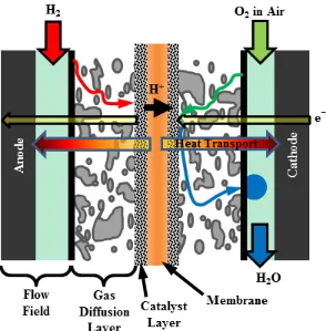
Figure 2: Schematic of PEMFC components and transport processes.
Proton Exchange Membrane (PEM): The main objective of this component is to transfer the hydrogen protons (H+) generated at the anode catalyst layer (CL) to the cathode CL. Meanwhile, the membrane should prevent the transport of any other species. The membrane consists of a hydrophobic and inert polymer structure that is sulfonated with hydrophilic acid clusters to provide proton conductivity [13]. Hydration of the membrane is required for proton conductivity. Hydration can be achieved through the presence of liquid water by the membrane. However, the amount of hydration should be optimized to prevent dehydration and water flooding in the adjacent layers. The typical thickness of a PEM can range between 18-25 μm and the PEM can resist temperatures up to 120 °C [13]. However, their operational temperatures do not exceed 90 °C [13] to ensure sufficient hydration.
6
are transported. This layer is a 3D porous structure with a typical thickness of 5-30 μm [13]. The porosity of CL is in between 0.4 and 0.6 [13] that is aimed to be increased for less resistance to mass transport. In order to reduce the electrical resistance, carbon and catalyst particles are bonded together. The ionomer has a fraction up 30% [13] to promote ion transport to/from the PEM. The removal of excess water is another issue to be considered because the CL mostly consists of hydrophilic materials. The hydrophilicity is balanced out by the partial use of hydrophobic polytetrafluouroethylene (PTFE).
Gas Diffusion Layer (GDL): This major role of this component is the uniform reactant transport to CL from the reactant channels and the product water removal from CL to reactant channels. This layer is made of either woven carbon cloth or nonwoven fiber paper as the macroporous layer, and a highly hydrophobic microporous layer (MPL) [13]. The thickness of GDL can range between 175 and 450 µm [13]. The hydrophilic carbon constituent leads to the possibility of water flooding that is prevented by the use of PTFE additive. Electron conduction to/from CL takes place through GDL. The electron resistivity for a given direction is dependent on the GDL type and PTFE content. Additionally, GDL transfers heat from the heat generation sites (CL and PEM) to the bipolar plate (BPP). The thermal conductivity is dependent on the PTFE fraction. Lastly, it provides mechanical support for PEM.
Microporous layer (MPL) is a complementary layer of the GDL. It is 5-20 μm thick and it has 100-500 nm pores [13]. MPL is used for water management because it is highly hydrophobic. In addition to water management, it is used to improve electrical conductivity between the CL and GDL, and prevent CL from carbon fiber intrusion damage caused by GDL.
7
are adjacent to each other at this particular BPP. As a result of the cell connections in series, a particular BPP is the anode and the cathode of two neighboring cells. It has a minimum thickness of 2 mm [13] which is much larger than the characteristic thicknesses presented for other components. The flow field may consist of parallel or serpentine channels. Serpentine configuration imposes a given air flow rate and hence, any water feature in the channel is discharged for whatever cost of pressure drop [15]. On the contrary, parallel channels are connected to the same manifold. Hence, a water feature in a channel can create flow resistance and the flow through the blocked channel can be directed to other parallel channels. Although parallel channels require less pressure drop than serpentine channels, they are prone to flow maldistribution [15].
1.2.2.
PEMFC Operation Principles
The fuel (hydrogen) and oxidizer (oxygen in air) are introduced into the cell through the anode and cathode flow fields, respectively. While the reactants run through the flow fields, they diffuse through their respective GDL and reach CL where the electrochemical reactions take place. The global reaction and the half reactions taking place at the CLs are:
Global: 2H2+ O2→ 2H2O (1)
Anode: 2H2→ 4H++ 4e− (2)
Cathode: 4e−+ 4H++ O
2→ 2H2O (3)
8
∆Γ = ∆Π − 𝑇∆Θ (4)
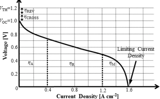
A typical performance measure of a fuel cell at steady state is the polarization curve. Figure 3 shows a typical polarization curve that plots the voltage (V) versus current density (i). In Figure 3, sections are identified to show the major sources of voltage loss (η). Although the sections are affiliated with a certain type of voltage loss, most of those regions are still under the partial effect of other voltage losses.
If all of the chemical energy in hydrogen could be transferred into electrical energy, the resulting electrical energy would equal to the change in enthalpy during the reaction (ΔΠ). The open circuit voltage (VOC) obtained in this hypothetical condition is named thermal voltage (VTH).
As the first source of voltage loss and heat dissipation, TΔΘ in Eq. (4) is an inevitable one due to
the nature of the energy conversion system. This loss is called reversible (ηREV) or Peltier loss.
9
Figure 3: A typical PEMFC polarization curve that is associated with voltage losses (η).
As the cell departs from the open circuit voltage, the electrons and protons are forced to displace due to the voltage difference between the CLs. The cathode always has a higher absolute voltage than the anode. This voltage difference is at its maximum during the open circuit condition. As the system operates at higher currents densities, the absolute voltages of cathode and anode are decreased and increased, respectively. This change leads to a smaller voltage difference between them as the current density increases. The loss of the voltage difference is used as the activation energy at the CLs and named as the activation loss (ηA). The activation loss
also incorporates the effect of fuel cross over through the membrane. The fuel cross over loss
(ηCROSS) is itemized separately only in the open circuit voltage condition when the activation loss
is zero.
The hydrogen protons (H+) and electrons are subjected to ohmic resistance that leads to ohmic voltage loss (ηR). Since the proton resistance dominates over the electron resistance, this
10
with hydrogen protons during cell operation [13]. This causes a water flux in the direction of proton transfer, namely from the anode to the cathode. This process is called electro-osmotic drag and is responsible for putting the anode side of PEM under the danger of dehydration. The diffusion and electro-osmotic drag of water counteract to each other and their net effect can be interpreted through the ohmic losses.
In addition to the proton conductivity of PEM, electron conductivity of the remaining layers plays a minor role in ohmic losses. The contributors to electron resistance are the CL, GDL, BPP, and the external load circuit. The last contributor to the ionic and electronic resistances is contact resistance between the layers, and it is due to the imperfect contact of two dissimilar materials.
As the current density approaches the limiting current density, the dominating voltage loss is the reactant transportation limitation or concentration loss (ηM). As the current density increases,
the reactant concentration difference between the flow field and the CLs has to become larger to sustain the required reactant flux. However, the reactant concentration in the flow field is constant for a given point and the concentration at the CL can be reduced to as low as zero. Under these circumstances, the available maximum concentration difference limits the maximum attainable current density. When the reactant concentration at the CL is low, the CL spends more energy to incorporate the scarcely available reactants into the reaction. This loss manifests itself in the high current region of a cell in the form of a dramatic voltage drop. This proposal focuses on the concentration losses taking place on the cathode side for the oxygen transport since the anode side losses are negligible comparably.
1.2.3.
Two-Phase Flow in PEMFC Components
11
GDL. The liquid and vapor states of water are transported from CL to reactant channels through different ways.
The vapor transport in the cathode GDL is governed by the concentration gradient of vapor in the air. This gradient is due to the higher vapor concentration at CL with respect to the reactant channel. The higher vapor concentration at CL does not necessarily stem from the aforementioned water production. As shown in Figure 4, the heat generation at PEM and CLs creates a higher temperature at the cathode CL with respect to the cathode reactant channels. The temperature gradient from CL to reactant channels leads to a vapor concentration gradient even when the air is fully humidified everywhere in the cell. Since the water saturation pressure increases non-linearly with the temperature, the air can carry significantly more vapor as temperature increases. Hence, the vapor transport in fuel cell porous medium can be mostly called thermal-gradient-driven. The transported vapor leaves the GDL from its reactant channel interface as shown in the center section of Figure 4.
12
Figure 4: Pressure gradient and thermal-gradient driven water transport mechanisms for liquid and vapor states, respectively. Porous gas diffusion layer and flow field are shown.
The water transport mechanisms affect the distribution of liquid water in the GDL. These mechanisms can be demonstrated through the visualization of the GDL liquid water distribution in an operational PEMFC. Figure 5 shows images of X-ray tomographic microscopy from a cell operating at 0.45 A cm-2 [19]. Vapor transport leads to condensation consistently underneath the BPP lands. Liquid water broke through the GDL into the reactant channel in the form a droplet. The droplet that emerge into the channel can later grow or coalesce with other and form more complex liquid water features such as films or slugs that will be discussed in the consequent sections.
Figure 5: X-ray tomographic microscopy of PEMFC cathode components (GDL and BPP) operating at the current density: 0.45 A cm-2 [19]. Visualized components: a) BPP, GDL and all liquid water; b) GDL and all liquid water; c) The water column connecting water generation site to the droplet.
1.2.4.
Transport of Oxygen in a PEMFC
[image:30.612.246.426.74.174.2]13
is less of a concern compared to the oxygen concentration owing to the higher diffusivity of hydrogen than oxygen. Oxygen concentration at the cathode CL is a function of concentration losses distributed from the air channel to the CL. These losses are located at GDL-channel interface, GDL, and GDL-CL interface. They depend on liquid water occupancy of the porous media. Hence, knowing the capacity of vapor removal through the porous media is important to predict the condensation in the pores and so, the oxygen concentration drops.
Oxygen concentration decreases along the flow direction in the channel due to continuous oxygen consumption. In order to minimize the variation of oxygen concentration in the flow direction, air flow rate is set to a value that provides more oxygen than to be consumed per unit time. The ratio of the volumetric air flow rate at the channel inlet to the volumetric air consumption is called stoichiometry (stoichiometric ratio). Most frequently, stoichiometry is set to be two in most PEMFC applications. At a stoichiometry of two, the oxygen concentration would reach half of its original value from the channel inlet by the channel outlet.
14
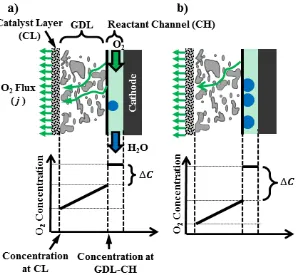
Figure 6: Concentration losses of oxygen during its transport from the reactant channel to the catalyst layer. Cases presented for a) fewer and b) more droplets in the channel.
The effect of two-phase flow in the reactant channel on the interfacial oxygen concentration drop is demonstrated by the comparison of Figure 6a and Figure 6b. The larger number of droplets in the channel covers a larger portion of the GDL-reactant channel interface. Hence, a larger concentration drop occurs. The variation of concentration drop is not only dependent on the area coverage of the interface by the droplet. Since the droplet changes the local air flow conditions, the transport resistance at the interface needs to be investigated.
1.2.5.
Oxygen Transport Resistance at the GDL-Air Channel Interface
[image:32.612.184.480.75.350.2]15
oxygen diffusivity in the air (𝐷O2−air) and hydraulic diameter (dh). The mass transfer coefficient
is non-dimensionalized with the aforementioned parameters into Sherwood number (Sh) which is independent of the parameters. Sherwood number is only dependent on the channel cross sectional aspect ratio and the boundary condition of mass transfer.
Possible scenarios of boundary condition are demonstrated in Figure 7. Both side walls and the top wall do not contribute to mass transfer. The bottom GDL-channel interface is subjected to oxygen flux. There are three possible conditions that can be seen at the interface during oxygen flux. Air may flow into or out from the interface, or the air may have zero velocity at the interface. Air flow into the interface is referred to as suction, while the flow out from the interface is injection.
Figure 7: Three scenarios of air velocity at the GDL-reactant channel interface depending on the relative amounts of water vapor and oxygen flux.
The relative amount of vapor and oxygen fluxes at the interface determines what air velocity the GDL-channel interface will have. If all by-product water is in liquid state, the interfacial air velocity will be dominated by the inward oxygen flux and this would result in air suction. If all by-product water is in vapor state, vapor exhaust can overpower the oxygen consumption and this would result in air injection. At conditions that vapor and oxygen fluxes are the same, the net air flow velocity becomes zero. As the boundary condition changes due to variable oxygen and vapor fluxes, Sherwood number can be affected and needs to be investigated.
16
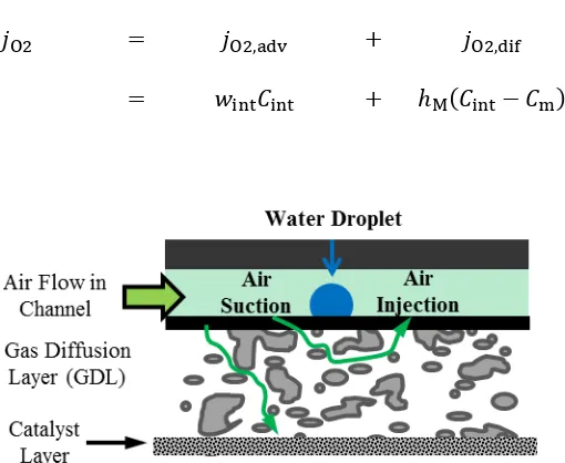
the flow can permeate into the GDL adjacent to the channel as shown in Figure 8. In conditions like this oxygen flux at the GDL-air channel interface (jO2) has advective (jO2,dif) and diffusive
components (jO2,dif) as shown in Eq. (5). The advective transport takes place at the interface with a
velocity of wint and O2 concentration of Cint. Diffusive transport is a function of mass transfer
coefficient (hM) and the difference between the mean O2 concentration in the channel (Cm) and Cint. In a simulation approach of neglecting the GDL and just simulating the channel, advective
transport at the interface is assumed to be zero. Simulations that incorporate the GDL can reveal the comparison of jO2,adv with respect to jO2,dif.
𝑗O2 = 𝑗O2,adv + 𝑗O2,dif (5)
= 𝑤int𝐶int + ℎM(𝐶int− 𝐶m)
Figure 8: Air permeation into the gas diffusion layer (GDL) due to a droplet. Air suction and injection take place upstream and downstream of the droplet, respectively.
[image:34.612.209.464.289.498.2]17
CHAPTER 2.
BACKGROUND
2.1.
TWO-PHASE FLOW DEPENDENT FUEL CELL PERFORMANCE
The performance of a PEMFC is investigated in the literature as a function of the liquid water in its reactant channels. Experimental and numerical studies are utilized to reveal the two-phase flow impact on the cell performance.
2.1.1.
Experimental Evidences of Performance Variations
Fuel cell experimentations mostly demonstrate the effect water slugs that plug the channels on cell performance [20]–[23]. It is frequently observed that as the current density is reduced, liquid water coverage in the channels increases [24]–[27]. This can be explained with the consideration of the following facts: Superficial air velocity and water production rate depend on the current density linearly. The drag force applied by the air flow on a water feature depends on the superficial air velocity quadratically. The quadratic dependence is due to the fact that the order of magnitude for a typical Reynolds number in the reactant channel is two. The volume of liquid water in channel increases with current density. The adhesion force of water features grows linearly with the feature size. Therefore, the adhesion of water features increases linearly. Linear and quadratic dependencies of water feature adhesion and the drag forces, respectively explains the reason of observing water features mostly at low current densities.
18
transport of air to the CL. This scenario is representative of serpentine reactant channels. In the case of parallel reactant channels connected to the same manifold, a slug in a channel can block the air flow to the respective channel completely. The air supplied from the manifold is redistributed to the unblocked parallel channels [28]. Since air convection is not present in the blocked channel anymore, mass transport cannot happen from that channel to the CL. In this case, interfacial resistance is irrelevant again. Therefore, interfacial resistance should be investigated for droplet and films but not for slugs.
The air flow can coexist with films and droplets in a channel. Some of the GDL-air channel interface remains unblocked and subjected to mass transfer. The interfacial transport resistance increases along with the reduction of interfacial area. Moreover, these water features alter the local flow conditions and change the way air flow interacts with the GDL-channel interface. Hence, Sherwood number is expected to change locally. The change in Sherwood number should be characterized to understand the effect of films and droplets on the cell performance.
2.1.2.
Numerical Evidences of Performance Variations
Numerical studies investigate how the variation of O2 resistance affects the cell performance.
Compared to experimental studies, numerical studies can reveal the impact of varying O2
resistance more clearly since they compare a channel with single-phase gas flow assumption and another channel with a realistic phase flow. Ding et al. simulated a 3D air channel with two-phase flow and the channel was coupled with a 1D membrane electrode assembly model at the GDL-air channel interface [29]. The effect of water slugs on the cell performance was studied. It was showed that slugs can increase the O2 transport resistance and decrease the cell voltage at
19
The effect droplet and films on cell performance was numerically studied by Chen et al. [30]. In their model, they simulated an air channel (0.28 mm × 0.34 mm × 2.00 mm) and a GDL as 3D domains, and a cathode CL as a boundary on the GDL. Figure 9 presents the simulated domains and a typical instant of droplet detachment. Compared to the model of Ding et al. [29], simulating the porous GDL in 3D allowed the air to permeate into the GDL in the flow direction in case of a droplet obstructing the flow. The cell was simulated at a voltage and average current density of 0.5 V and 1.92 A cm-2. It was shown that the permeation of air flow under a sliding droplet on the interface can increase the local current density. The average current density was shown to increase 10 mA cm-2. Moreover, a film at the top channel wall (across the GDL-channel interface) could also increase the local current density as it directs the air flow towards the GDL-channel interface. However, the positive and local impact of the film is not significant enough to increase the average current density. In order to complement the studies by Ding et al. [29] and Chen et al. [30] revealing the effects of two-phase flow patterns, there is a need to characterize the local interfacial O2 resistance for PEMFC operating conditions.
20
2.2.
CONSIDERATIONS OF INTERFACIAL MASS TRANSPORT
RESISTANCE IN PEMFC PERFORMANCE MODELING
2.2.1.
Models Implicitly Solving for the Interfacial Resistance
In numerical models of PEMFCs, GDL and reactant channels should be simulated together for the interfacial oxygen transport resistance to be calculated and incorporated into the results. Fluid flow and mass transport equations should be solved in these domains. In these models, the computational requirements become significantly demanding compared to the ones omitting the simulation of flow in reactant channels. The advantage of simulating the reactant channel is that they can simulate the interfacial phenomena with higher fidelity to reality since the GDL and channel are coupled. Although these models simulate the interfacial transport resistance, this phenomenon is incorporated into the performance prediction results implicitly and the resistance values are not reported explicitly.
There is a wide range of 3D wet PEMFC modeling studies which incorporated the full solution of gas flow in PEMFC flow fields along with electrochemistry equations [31]–[41]. Figure 10 shows an example 3D meshed domain for a PEMFC model [32]. This numerical model incorporates the anode and cathode sides. Two reactant channels on each side represent a portion of serpentine flow fields. However, the bents of the serpentine flow fields were neglected in this model and flow switched direction as it advances in the vertical direction. The meshed domain shows that the reactant channels require a significant number of mesh elements. Hence, the complexity of the cell model is increased significantly to simulate the channels.
21
Figure 10: An example of a 3D wet PEMFC model that simulates the PEM, CL,GDL and serpentine reactant channels at anode and cathode sides [32].
[image:39.612.254.414.75.237.2]22
could not be applied. Moreover, these studies did not report the mass transport resistance which was implicitly solved in the numerical models.
2.2.2.
Models Incorporating the Interfacial Resistance as an Input
Parameter
In the literature, simplified PEMFC models utilize the Sherwood number as a constant input to save computational resources from the simulation of forced convection in the air channels [44]–[57]. The constant input of Sherwood number is a valid assumption if the flow is fully developed in the reactant channels, such as the absence of liquid water features in high temperature PEMFCs [54]. However, the constant Sherwood number assumption is not always applicable. Kim et al. shared a similar anticipation that the Sherwood number might depend on specific fuel cell operating conditions and configurations [47]. Casalegno et al. [52] in 2010: “The correlations to determine the Sherwood number in the two-phase flow conditions, …, are not available in the literature.”.
2.3.
INVESTIGATION OF INTERFACIAL MASS TRANSPORT
RESISTANCE
2.3.1.
Utilization of Heat and Mass Transport Analogy
23
numbers are the same. In case Sc and Pr are different from each other, the mapping between Sh and Nu should be investigated for specific cases in the PEMFC air channel.
With the use of ShFD, a preliminary calculation can be made to show the relative importance
of interfacial O2 transport resistance with respect to the resistance through the GDL. For the air channel cross section in interest in this study (0.70 mm × 0.40 mm), using the heat and mass transfer analogy leads finding the value of ShFD to be 3.349. Based on the technique that will be
presented in Section 5.1.1.5. , the concentration drop at the interface and through the GDL is calculated to be 0.65 and 0.33 mol m-3, respectively at the current density of 1.5 A cm-2.
2.3.2.
Simulation of the Interfacial Transport Resistance
Since the research on the Sherwood number in PEMFC reactant channels has not yet been very well established, only a few numerical simulations are available in the literature. These studies have 2D (parallel plates) and 3D approaches. The results by the 2D models do not reflect realistic results due to fact that PEMFC reactant channels typically have an aspect ratio close to unity. All these studies investigated the effect of air injection/suction at the GDL-air channel interface on the Sherwood number. Depending on the intensity of suction or injection, the flow may remain developing in the channel. Under developing flow conditions, the Sherwood number can vary and hence, has been a subject of investigation.
24
These findings allow the simulations to neglect any injection or suction at the GDL-reactant channel interface. However, the previous studies neglected the effect of liquid water present in the channel on the Sherwood number.
2.4.
REACTANT CHANNEL TWO-PHASE FLOW PATTERNS
In order to study the effect of liquid water features on Sherwood number, visual characterization of the water features is required. After characterizing the shape, size, and motion of the water features, these features can be incorporated into simplified models as obstructions to single-phase gas flow without the need of simulating the complex two-phase flow. The liquid water present in the reactant channels can be characterized through visible-light-transparent PEMFC designs. These are called in-situ experiments since they use an operational fuel cell. The use of visible light provides high spatial and temporal resolution compared to other options, such as X-ray radiography, neutron radiography, and magnetic resonance imaging [64].
In order to control the two-phase flow conditions more accurately, operational fuel cells are transformed into ex-situ experiments that introduce the liquid water into reactant channels through artificial injection [26], [65]. Moreover, there are dedicated fundamental microfluidics studies on droplets, films, and slugs [66]–[71].
2.4.1.
In-Situ Visualization of Two-Phase Flow
The two-phase flow visualization in operational PEMFCs has been conducted to observe changes in flow conditions locally in the cell and in response to varying operating conditions. Tüber et al. conducted one of earliest visualization studies by the use of a PEMFC that is as wide as a single reactant channel [55]. Kimball et al. [23] and Dillet et al. [22] experimentally correlated the motion of slugs and changes in local current density.
25
maldistribution. Moreover, flooding water volume for the channels was reported as a figure of merit for flow field designs. Masuda et al. compared flow field designs of single and three parallel, and three serpentine channels [21]. The designs are compared through pattern of voltage fluctuations due to two-phase flow.
In-situ experiments are utilized to establish correlations for the movement of an individual water feature. Yang et al. [73] and Ous and Arcoumanis [74] experimented with PEMFCs utilizing multiple parallel channels and a serpentine channel, respectively. These works mostly focused on droplets and their patterns of growth and departure. Zhang et al. used a PEMFC with multiple parallel channels [75]. They observed droplets, films and slugs. They also built a correlation for the droplet detachment diameter for the tested range of superficial air velocities. Spernjak et al. used serpentine channels and varied the temperature [76] They reported that the superficial gas velocity of 7.4 m s-1 led to droplets readily detached in channels with the cross section 0.8 mm × 1.0 mm. Zhan et al. showed that liquid water is removed easily for air velocity larger than 7 m s-1 in a channel cross section of 1.5 mm × 1.5 mm [24].
26
[image:44.612.243.420.351.531.2]The local air flow conditions in the vicinity of a droplet are altered as a function of droplet emergence location along the channel width. It is known that droplets mostly emerge from under the bipolar plate (BPP) lands (ribs) [16], [17]. However, there are studies suggesting that this does not always have to happen. Optical visualization studies documented that the droplets can emerge in the center of the channel width [27], [73], [75], [77], [78]. It was hypothesized that a GDL with a smaller porosity would lead to a droplet emergence more uniformly distributed along the channel width rather than concentrated underneath the BPP lands [79]. As shown in Figure 11, it was proposed to have a groove in the GDL at the channel center width and along the flow direction to create a preferential droplet emergence location and hence increase the cell performance [80]. Based on these observations, droplets can emerge from the channel side wall-GDL corner and wall-GDL-channel interface center width.
Figure 11: A PEMFC with a grooved GDL that leads to water droplets emerging from the channel center width.
2.4.2.
Ex-Situ Visualization of Two-Phase Flow
27
fundamental experiments by not focusing on a specific water feature but the overall result of water features-air flow interaction.
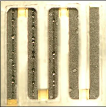
Le et al. used a serpentine channel design for ex-situ testing and simulating the two-phase flow numerically [65]. The liquid water was injected through a single pore in the vicinity of air channel inlet. The areas prone to flooding were identified. The experimental and numerical results agreed well. Banerjee and Kandlikar used a parallel channel flow field with variable temperature and relative humidity [26]. Similar to a previous study [25], the area coverage ratio was quantified in terms of films and slugs. As an additional contribution, this ratio was quantified at each channel separately. In all values temperature and relative humidity, area coverage ratio decreases consistently with equivalent current density. For a constant current density, the area coverage ratio was observed to decrease with temperature and relative humidity.
2.4.3.
Fundamental Experimental Studies on Two-Phase Flow Patterns
Fundamental studies focus on the motion of two-phase flow pattern components, such as a droplet, film, and slug. These studies attempt to recreate the conditions that a water feature would be subjected to in a fuel cell and understand how the water feature behaves when one variable is changed at a time.
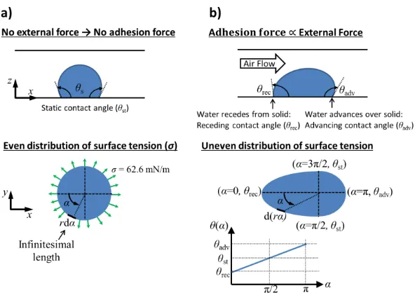
28
Figure 12: Contact angle distribution on the perimeter of a droplet foot print, under conditions of: a) absence of an external force, b) presence of an external force.
The contact angle of a droplet varies when it is subjected to external forces as shown in Figure 12b. The adhesion force of the droplet to the solid as a reaction force is dependent on how uniform the contact angle distribution will be at the droplet foot print perimeter. The non-uniform distribution of contact angle leads to a non-zero net force on the solid plane. The droplet foot print can be divided into two halves. The half that is further to the direction of external force has a contact angle larger than the static contact angle. The maximum value of contact angle on this side is called advancing contact angle (θadv). On the other half of droplet footprint, the contact
angle values become smaller than the static value. The minimum contact angle on this side is called the receding contact angle (θrec). The adhesion force of the droplet increases with the
difference between advancing and receding contact angles. This difference is called contact angle hysteresis.
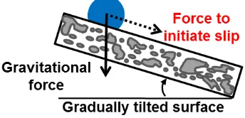
29
measured as in Figure 13 by the help of a tilted surface with a droplet placed on it. Once the tilt angle exceeds the threshold value and droplet starts to accelerate, the dynamic contact angle hysteresis can be measured. Static contact angle hysteresis for carbon paper was shown to be larger than the dynamic one.
[image:47.612.242.414.303.386.2]Das et al. measured the droplet deformation under gravity and measured the force to initiate sliding in static conditions [70]. The droplet deformation under gravity was reported to be negligible for Bond number (Bo) values under 0.1. Moreover, static contact angle hysteresis and the resulting adhesion force were measured at various GDL samples, including aged ones.
Figure 13: Static and dynamic contact angle measurement setup utilized by several researchers in the literature.
Droplets in a channel are deformed due to the air flow around them. The deformation increases proportional to the intensity of air flow inertia, hence the superficial air velocity. Cho et al. experimentally correlated this droplet deformation [82], [83]. The deformed shape can be expressed as an ellipsoid with a semi-major axis of rx and a semi-minor axis ry. The mismatch
between the two semi-principal axes is normalized with the average droplet radius (ry - rx) / r as
30
Figure 14: Characterization of droplet deformation through the mismatch of droplet diameter measured in two normal axes.
The droplet in an air flowing channel has a recirculation inside due to shear forces acting on the droplet-air interface. By characterizing this recirculation, the velocity at the droplet-air interface can be extracted. Minor et al. used micro digital particle image velocimetry technique to quantify droplet internal circulation [84]. Figure 15 shows the droplet in the absence and presence of air flow with the use of particle image velocimetry technique. In a channel cross section of 1 mm × 3 mm, the maximum superficial air velocity was 6.000 m s-1
which corresponded to a channel based Reynolds number of 580. The maximum velocity in the droplet was recorded to be 0.105 m s-1 which is 1.75% of the superficial air velocity. Hence, droplet surfaces under air flow can be assumed to have zero velocity.
Figure 15: A droplet emerging from a GDL into an air channel: a) No air flow in the channel; b) Air flow in the channel leads to luminescent particles creating streaklines in long exposure.
31
volumes of the slugs formed were correlated with superficial air and water velocities. Cheah et al. [86] expanded on the work of Colosqui et al. [85] by experimenting with different channel surface energies and cross sections. The following understanding was shared as a result of the experiments: The mass transport losses increase with slug length. However, a slug divided into smaller compartments will need more energy to be removed since there is more interfacial area to create adhesion due to surface tension forces.
32
CHAPTER 3.
OBJECTIVES
The objective is to obtain oxygen transport resistance at the GDL - air channel interface under two-phase flow conditions. The transport resistance is expressed with the non-dimensional Sherwood number and needed in simplified PEMFC performance models. Two-phase flow conditions refer to the presence of water droplets and films. Characterization of Sh in the vicinity of water droplets and films can lead to more accurate predictions in the performance models. Sherwood number needs to be characterized as a function of distance along the flow direction, water feature size, spacing, and fuel cell operating conditions, such as current density, stoichiometry, temperature, and relative humidity. Numerical simulations should be used to obtain local variations of Sh with the aforementioned parameters. The results should ultimately be expressed through mathematical correlations that can be conveniently used by PEMFC performance models. This main objective can be divided into smaller components as below:
3.1.
OBTAINING THE TRENDS OF SHERWOOD NUMBER AS A
FUNCTION OF DROPLET AND FILM CONFIGURATION BY USING
NUMERICAL SIMULATIONS
This study aims to minimize the computational cost of simulating the effect of droplets and films on Sherwood number. For doing so, it is proposed to use obstructions shaped like water features to partially block the single-phase air flow in a channel. The use of obstructions requires the knowledge of water feature shape, detachment conditions, and water-air boundary conditions. Fundamental microfluidics studies already documented the shapes of droplets and films under air flow that is equivalent to conditions in PEMFC air channels. These shapes can be approximated in a simulation through the sum/subtraction of basic geometrical shapes, such as spheres, cylinders, and rectangular prisms.
33
provided in the literature. By comparing the adhesion force from the literature to the drag forces numerically computed, only cases that lead to water feature adhesion can be simulated.
At the interface between air and water, the fluid velocity needs to be known to impose the proper boundary condition on the water feature obstruction. In reality, air flow and water within the droplet are coupled in motion. Since the use of obstructions decouples the motion of two-phases, experimental documentation of droplet internal recirculation needs to be utilized.
3.2.
BUILDING CORRELATIONS FOR SHERWOOD NUMBER
The results of Sherwood number in the vicinity of water features are expected to show trends with the variables to be simulated. The aim is to build non-dimensional mathematical correlations to be used in simplified PEMFC performance models. These correlations should reflect the changes in the flow direction and operating conditions. Separate correlations needs to be built for droplets and films. These correlations should be in non-dimensional for them to be used at a wider range of conditions and length scales. These correlations can be used along with the visualization data of operational PEMFCs. The statistical distribution of water features in a channel can indicate where to use the Sherwood number correlations. Therefore, the correlations should be built to be comprehensive enough for the possible visualization outcomes.
3.3.
EXPANDING
THE
USE
OF
SHERWOOD
NUMBER
CORRELATIONS
34
35
CHAPTER 4.
APPROACH
4.1.
PHYSICAL MODEL
The air properties were kept constant in the simulations and calculated at the temperature (T) and relative humidity (RH) of 80 oC and 100%, respectively. The density (ρ) and dynamic viscosity (µ) of the air were calculated from the correlations provided by Tsilingiris [88]. The diffusivity of oxygen in the air (DO2-air) was approximated based on the molar-averaged
diffusivities of major air constituents within each other [89]: oxygen, vapor, and nitrogen. The constituent molar fractions and diffusivities were calculated with correlations by Mench (saturation pressure of vapor) [13] and Fuller et al. [90], respectively. With the use of the aforementioned air properties, Schmidt number (Sc = µ ρ-1 DO2-air
-1
) was calculated for a temperature range from 0 to 80°C. Table 1 shows all the air properties mentioned above as a function of temperature.
Table 1: Properties of fully humidified air for the temperature range from 0 to 80°C: mass density (ρ), dynamic viscosity (µ), and Schmidt (Sc) number.
T [°C]
ρ [kg m-3] µ [µPa s] DO2-air [cm 2
s-1] Sc
0 1.293 17.157 0.174 0.762
20 1.194 17.958 0.200 0.753
40 1.100 18.374 0.227 0.735
60 0.987 18.034 0.262 0.699
80 0.828 16.253 0.310 0.632
![Figure 1: Various currently available energy-well-to-drive-wheel chains for a transition to hydrogen use as an energy medium (adapted from [1])](https://thumb-us.123doks.com/thumbv2/123dok_us/94474.8882/20.612.141.497.460.670/figure-various-currently-available-energy-transition-hydrogen-adapted.webp)
![Figure 5: X-ray tomographic microscopy of PEMFC cathode components (GDL and BPP) operating at the current density: 0.45 A cm-2 [19]](https://thumb-us.123doks.com/thumbv2/123dok_us/94474.8882/30.612.246.426.74.174/figure-tomographic-microscopy-cathode-components-operating-current-density.webp)
![Figure 10: An example of a 3D wet PEMFC model that simulates the PEM, CL,GDL and serpentine reactant channels at anode and cathode sides [32]](https://thumb-us.123doks.com/thumbv2/123dok_us/94474.8882/39.612.254.414.75.237/figure-example-pemfc-simulates-serpentine-reactant-channels-cathode.webp)