(
LIBRARY jA thesis submitted for the degree of DOCTOR OF PHILOSOPHY
of the
AUSTRALIAN NATIONAL UNIVERSITY
by
STATEMENT
This thesis is an account of my research undertaken during the period March 1986 to December 1989, while I was a full-time student in the Research School of Earth Sciences at the Australian National University.
Except as otherwise indicated in the acknowledgements and in the text, the work described is my own.
This thesis has never been submitted to another university or similar institution.
David Carl Jepsen Canberra,
ACKNOW LEDGEM ENTS
Throughout the course of this research I have been fortunate enough to work with and meet many people who have encouraged me in my research over a 4 year period. I hope the following few words fully extends my appreciation to them.
I sincerely wish to thank my supervisor Dr. B.L.N. Kennett for his constant guidance, advice and encouragement throughout the course of this study, for whom this work would not nave been completed. I thank my fellow colleagues in the Seismology Group : M. Bostock, S. Cao, D. Christie, S. Dey, B. Goleby, J. Grant, G. McAllister, W. Penders, T. Percival, M. Sambridge and J. Weekes, who have provided a friendly environment inducive to research. I have also benefited from many discussions within the group. Special thanks go to Robert Dabrowski for sorting out many of my computing difficulties. The criticism of the research work by P. Cummins is also greatly appreciated. Jan Hulse provided me with an escape route from many of my problems, which was quite entertaining at times, and I fully acknowledge his warmth and friendship.
The 3 weeks I spent at Flinders University, Adelaide with Dr. S. Greenhalgh and his colleagues is much appreciated as it gave me an insight for analysing 3-component data. I would also like to thank T. Kvasma who provided me with Noress and Arcess seismic data and several analysis programs.
The financial support from the Department of Employment, Education and Training, the University Grants Committee, Victoria University, and my parents is gratefully acknowledged.
This thesis develops data processing techniques for multi-component seismic array data which are designed to exploit the physical character of the seismic signals.
For an array of single component seismometers I have developed a beamform scanning technique and I have improved the adaptive processing method developed by King et al. in 1973, for the simultaneous estimation of horizontal slowness and azimuth of the signals. These techniques have been applied on a set of earthquakes from the Indonesian-New Guinea region recorded at the Warramunga and Rockhampton Downs arrays in northern Australia, in an attempt to study source and receiver heterogeneity. It was found that heterogeneity exists on different scale lengths and the scale length of heterogeneity increases with depth.
To further improve our understanding of the velocity structure and the degree of heterogeneity within the earth I have developed several methods for the analysis of 3-component data. Conventional approaches to the analysis of 3-component seismic records endeavour to exploit the apparent angles of propagation in the horizontal and vertical planes and the polarisation of the waves. The basic assumption is that there is a dominant wavetype (e.g. P waves) travelling in a particular direction which arrives at the seismic station in a given time window.
By testing a range of characteristics of the 3-component records it was possible to build up a set of rules for classifying much of the seismogram in terms of wavetype and direction. The application to events recorded at the Noress and Arcess arrays in Norway have shown that much of the coda is identified, and so implies that this process would be a reasonable tool for on-line phase identification. It is, however, difficult to recognise SH waves in the presence of other wavetypes, and the slowness vector could only be satisfactorily determined for P waves. Problems also arise when more than one signal (in either wavetype or direction) arrive in the same time window.
CON TENTS
Chapter 1 : Introduction 1
1.1 Characteristics of a seismic array 1
1.2 Purpose of a seismic array 2
1.3 Seismic array design 3
1.4 Previous types of array studies 6
1.5 Three-component analysis 8
1.6 Thesis outline 9
Chapter 2 : Single component array techniques 12
2.1 Processing techniques 12
2.1.1 Beamforming techniques 13
2.1.1.1 Linear stack 13
2.1.1.2 Semblance stack 15
2.1.1.3 Semblance enhanced stack 15
2.1.1.4 Nth root technique 16
2.1.1.5 Scanning technique 17
2.1.2 f-k process 18
2.1.3 Adaptive processing 19
2.1.4 Processing in the Tau-p domain 21
2.1.5 Discussion 25
2.2 Accuracy of techniques for upper mantle phases 25 2.3 Slowness and azimuth resolution of small and medium
aperture arrays 28
2.3.3 Noress and Arcess 30
2.3.4 Array response diagrams 30
Chapter 3 : Analysis of vertical component data recorded at
the Warramunga and Rockhampton Downs seismic
arrays 33
3.1 Near source heterogeneity 33
3.1.1 N. W. Irian Jaya 36
3.1.2 New Ireland/New Britain 39
3=1.3 Banda Sea 40
3.1.4 Cluster discussion 42
3.2 Receiver heterogeneity 44
3.2.1 Small scale heterogeneity 44
3.2.2 Large scale heterogeneity 45
3.3 Discussion 47
Chapter 4 : Three-component methods 48
4.1 The motion recorded on seismographs 50
4.2 Signal direction finding (SDF) techniques 53
4.2.1 Triax 53
4.2.2 LS 54
4.2.3 Power 55
4.2.4 Diff 56
4.2.5 Discussion 56
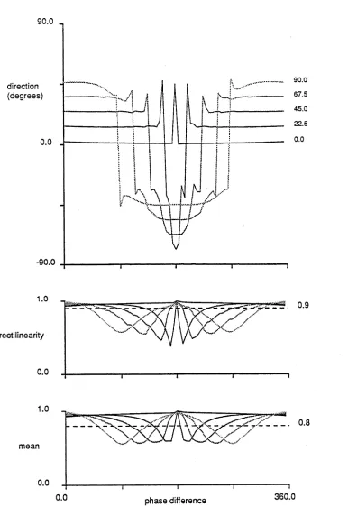
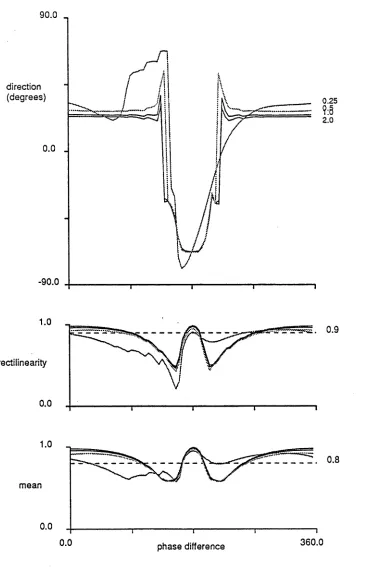
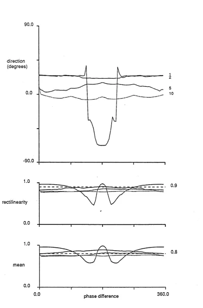
4.3 Phase difference polarisation technique 59
4.5 Wavetype discrimination 65 4.5.1 Waves with essentially rectilinear motion 65
4.5.2 Waves with 2D motion 67
4.5.3 3D motion 69
4.6 Application to synthetics 69
4.6.1 Teleseismic situation (single slowness plane
wave model) 71
4.6.2 Teleseismic situation (single slowness plane
wave model) with signal generated noise perturbations 72
4.6.3 Regional S wave seismograms 73
4.6.4 Regional S wave seismogram with simulation
of heterogeneity 74
4.6.5 Complete regional seismograms 76
4.6.6 Discussion 78
Chapter 5 : Three-component analysis 79
5.1 Application to single 3-component stations 80
5.1.1 Event Nor 1 81
5.1.2 Event Arc2 87
5.1.2.1 Arc2-P coda (8-30s) 88
5.1.2.2 Arc2-S coda (31-40s) 90
5.1.2.3 Arc2-Rayleigh wave (41-47s) 91
5.1.2.4 Arc2-later coda (48-70s) 92
5.1.2.5 Arc2-complete analysis 92
5.1.3 Conclusion 94
5.2 Application to an array of 3-component stations 96
5.2.1 Three-component stack 97
Chapter 6 : Wavefield decomposition 102
6.1 Near surface modelling 103
6.1.1 Frequency independent models 105
6.1.1.1 Infinite medium 105
6.1.1.2 Half-space 105
6.1.2 Frequency dependent models 108
6.2 Precision in the recovery of the amplitude vector 109
6.3 Application to real data sets 114
6.3.1 Event W 1186 116
6.3.2 Event Norl 117
6.3.3 Event Arc2 118
6.4 Discussion 119
Chapter 7 : D iscussion 120
Appendix 1 : Least squares estimation of slowness and azimuth 123
Appendix 2 : Hypocentre information (ISC) 126
1
Chapter 1
INTRODUCTION
1.1 Characteristics of a seismic array
Seismic arrays (the spatial arrangement of seismometers) were introduced in the late 1950’s to monitor underground nuclear explosions (see review paper by Davies (1973)). However their superior ability to detect, locate and identify seismic events compared with single station seismometers, arrays are now also employed to explore in more detail, lateral and vertical heterogeneities in the earth's velocity structure.
1.2 Purpose of a seismic array
Arrays are deployed to suppress uncorrelated seismic noise while preserving signals from seismic events, with the aim to obtain a signal to noise gain approaching Vm, where M is the number of sensors. If the signals on each sensor are identical and the noise is Gaussian and uncorrelated, the beamforming gain is proportional to VM (Johnson, 1968). In general, however, signals are not perfectly coherent across an array and signal generated noise in the form of multiple reflections and mode conversions give added complexity to the recorded signal, hence the theoretical VM gain is rarely achieved.
An array can be employed as a directional filter, i.e. the array can be steered in a certain direction by inserting time delays to the non-vertical incidence of a wavefront, in order to enhance signals from that direction. This allows the array to discriminate between signals and noise arriving from different directions. In this project this is achieved by inserting delays corresponding to various slowness-azimuth combinations and searching for an absolute maximum in the array response. Alternatively the direction can be estimated directly by effectively fitting a plane wavefront to the measured time delays of the signal of interest (Kelly, 1964). Deviations in the estimated values of azimuth and slowness occur due to the departure of the wavefront from the assumed plane wave configuration, but due to the nature of the signal wavelength and the array aperture, this really only concerns large aperture arrays. Array studies have shown that signal enhancement and array steering are important in :
3 location estimates by an array for distant events are poor, an array can locate weak seismic events and give much better estimates of local events.
(ii) Decomposing signals in terms of their frequency content, azimuth of arrival and slowness: an array has an advantage over single station seismographs as it can give a direct measurement of the slowness vector, and this eliminates many sources of error prominent in smoothed horizontal slowness (dT/dA) v distance (A) curves, such as hypocentre location and origin time, as the measurement is independent of absolute time (Johnson, 1967). Accuracy of these measurements is important as they are used to determine regional velocity structures.
(iii) Separating signals which arrive at the array simultaneously : triplications of the travel time curve can be closely spaced in time, but as their propagation characteristics are slightly different, arrays of sufficient aperture are able to separate them. Separation of phases is important as the more phases that can be clearly identified the better the velocity structure with depth can be resolved.
(iv) Determination of the seismic noise field : information on noise characteristics is important for seismic event detection and for future array development.
(v) Detecting weak signals : this is important in searching for phases that are difficult to observe. Ringdal (1985) and Souriau and Souriau (1989) have employed seismic array data to detect core phases, whereas Richards and Wicks (1990) have been able to analyse S-P conversions to study the characteristics of the 650km discontinuity.
1.3 Seismic array design
sensor spacing was greater than 2km (Davies, 1973). Consequently specially designed arrays with wider apertures were constructed and they preceded along 2 lines :
(i) United Kingdom Atomic Energy Authority (U.K.A.E.A.) medium aperture arrays. (ii) Large aperture arrays (aperture ~ 100km) such as LAS A, NORSAR and ALPA.
Since the extent of these arrays is comparable or larger than the signal wavelength, time delays need to be inserted before summing to account for signal propagation across the array, hence the arrays can be used as directional filters.
The U.K.A.E.A. arrays were built in the early 1960's and generally followed a standard configuration. Each array has 20 Willmore Mark II SPZ sensors arranged in an "L" or "T" shape (see Mowat and Burch, 1974) and their inter-seismometer spacing is between 2 and 2.5km (except EKA), which is a compromise between the decorrelation of surface wave noise and the limitation of the array aperture (King, 1974). The standard digitisation rate is 20Hz and the response is similar to WWSSN short-period sensors up to 2Hz (see Kennett, 1983), and above that frequency, the response is nearly flat to velocity. These arrays introduced the concept of steered beams and were designed to detect small P phases at teleseismic distances. A signal to noise improvement approaching Vm is obtainable, except when the noise is directional. Characteristic noise levels are quite different at the arrays, but the noise spectrum in general decays with an essentially linear slope from about 2Hz to the system noise limit of the array (Bache et al., 1986).
5 provide locations of events that are below the reporting threshold of ISC, and consequently can identify arrivals otherwise neglected (Ringdal and Husebye, 1982).
For large arrays there is a problem in attaining Vm improvement, this is not because the noise is coherent, but depends on whether the (short period) signal is coherent over such a distance. Depending on the degree of heterogeneity in the vicinity of the array, strong signal distortion may occur, which will limit the coherency of the waveform over the whole array. This problem can be rectified, as observed at NORSAR and LASA by having a denser sampling of seismographs at the centre of the array than on the flanks, so the signal can be coherent on more seismographs. Ringdal and Husebye (1982) found that the improvement in SNR at LASA and NORSAR is generally within 3 to 5db of the theoretical Vm gain. Although the signal coherence is not comparable to smaller aperture arrays, the inter- seismometer spacing of these arrays is large enough to resolve triplications.
The data accumulated at LASA and NORSAR has been used to study regional upper mantle velocity structures and characteristics of the seismic wavefield (Mack, 1969; Capon, 1969; Davies, 1973, and Berteussen, 1976), and complete descriptions of these arrays are given by Green et al. (1965) and Bungum (1971). Due to the cost of maintaining large aperture arrays and the problems in monitoring a nuclear test ban, only the NORSAR array still exists, but in a reduced format. Array analysis has now essentially reverted back to small and medium sized arrays.
capabilities of Noress in terms of regional detection, location and phase identification, but there are noticeable differences in their phase characteristics (Mykkeltveit and Ringdal,
1988).
Portable arrays like the NWB array discussed by Bowman and Kennett (1990) and those described by Muirhead and Hales (1980), are employed for regional studies, and their size and configuration are linked to the regional tectonics which are to be analysed. The arrays may employ variable inter-seismometer spacings so different parts of the mantle can be studied, and if the array is large enough it can also be used to detect the existence of major discontinuities within the earth's velocity structure, much like the large aperture arrays. Bowman (1988) suggested that when the portable NWB array is used in conjunction with the permanent Warramunga array, phase correlation across the array and among different earthquakes is possible.
Three-component arrays, in general, are incorporated with a vertical component array, e.g. at WRA, Noress, Arcess and shortly at Yellowknife. These arrays are employed to study polarisation characteristics of the seismic coda and to identify seismic phases (see section 1.5).
1.4 Previous types of array studies
7
these studies implicated a complicated structure, seismic arrays were shown to have greater resolving power, as accurate recordings could be made and precise measurements of the seismic propagation could be determined. Firstly, they provide direct measurement of the horizontal slowness (dT/dA) over a limited range of A, and thereby allow resolution of minor perturbations in the travel time curve, and secondly processing of array records results in SNR improvement, and so weak arrivals can be detected, which can then be included in the data which determines the travel-time curve.
Direct measurements of dT/dA have been employed to construct travel-time curves for various regions of the earth and consequently velocity models have been derived by inverting the data using the Herglotz-Weichert technique (e.g. Niazi and Anderson, 1965; Johnson, 1967, 1969; Chinnery and Toksöz, 1967; Wright and Cleary, 1972). All these types of studies realised the effect of local structure on azimuth and slowness measurements, and they attempted to account for this by assuming a crustal and upper mantle structure based on some previous information e.g. refraction models. Otsuka (1966b), Niazi (1966) and Underwood (1967) tried to account for large scale anomalies in terms of a dipping interface, however this method was found to be insufficient in describing the anomalies properly, so future studies employed travel-time residuals to calibrate the measurements (e.g. Cleary et al., 1968 and Wright, 1970). Simpson (1973) and King (1974) pointed out that the effect of local structure at WRA could not be eliminated, but the errors could be reduced by restricting the azimuthal range of the earthquakes so that the measurements vary only by a constant or slowly varying term. Datt and Muirhead (1976, 1977) and Hendrajaya (1981) employed this technique on selected earthquakes in the Indonesian-New Guinea region and they were able to refine previous models by also using later arrivals.
interpretation of data (Datt, 1981). Most of the velocity models proposed are complex, but they generally show the presence of a 400km and 670km discontinuity, and in some cases the existence of a low velocity zone. Direct slowness measurements have also been used to study the velocity structure as deep as the inner/outer core boundary (Johnson, 1969; Souriau and Souriau, 1989).
Although arrays are now primarily used to determine regional variations in the velocity structure, their original intention to detect and locate nuclear and seismic events is still of prime importance. Much of the study of NORSAR and Noress data lies in this field. In recent years array studies have also been involved in determining the degree and extent of heterogeneity (e.g. Kennett, 1987; Korn, 1988; Kennett and Bowman, 1990) and for the observation of earthquake rupture propagation and near source ground acceleration (Spudich and Cranswich, 1984; McLaughlin et al., 1983; Liu and Heaton, 1984).
1.5 Three-component analysis
In recent years seismologists have strived to obtain more information on the velocity structure of the earth and the propagation of seismic waves. One way this may be achieved is to decompose the wavefield into single wavetypes, identify them, and obtain an estimate of the associated slowness vector. From a single 3-component station, polarisation properties of recorded signals can be determined, as shown by Jurkevics (1988), and a direct measurement of the slowness vector in some cases can be calculated if the wavetype is known. On the otherhand, when the polarisation properties of the various wavetypes (purely polarised) are modelled for a particular medium (normally an isotropic medium), probability estimates for the presence of a given wavetype can be determined (e.g. Christoffersson et al., 1988).
9 the wavefield classification procedures break down. The scheme developed by Christoffersson et al. (1988) and the one developed in this thesis show that the P coda of an earthquake can be satisfactorily decomposed, but the waveform characteristics of the S coda are found to be quite complex, and so only parts of the coda are identified. Single 3-component station estimates are quite unstable, and Jurkevics (1988) showed that a direct sum of 3-component datasets improves the stability of these estimates, as the effect of signal generated noise is reduced in much the same way as beamforming techniques. Although techniques employing 3-component data can partially decompose the wavefield, no proper estimates (except for the initial P phase) of azimuth and slowness can be determined, so they are not viable methods for estimating propagation properties.
The ability of the 3-component data to identify seismic phases has been helpful in epicentre determinations (Ruud et al., 1988), and polarisation analyses are employed for the study of shear waves and anisotropy (Booth and Crampin, 1985; Cormier, 1984; Douma and Helbig,
1987). Three-component datasets have advantages over a vertical component array in that a sparse triaxial array is much cheaper and a single 3-component station does not require a large geologically uniform area.
1.6 Thesis outline
The aim of this thesis is to develop methods which can supply information on the propagation and polarisation characteristics of the seismic wavefield, which in turn can be used to resolve some of the finer details of the earth's velocity structure, and give a greater understanding of heterogeneity within the earth. The thesis will stress that much more information on the characteristics of the wavefield can be obtained if one models the interaction of seismic waves near the surface of the earth.
with array response diagrams which describe the accuracy in which signals can be resolved by the seismic arrays used in this thesis.
In chapter 3 several of these techniques are applied to a group of earthquakes in the Indonesian-New Guinea seismic zone in an attempt to study heterogeneity in the crust and upper mantle. Clusters of earthquakes throughout this region were chosen to study the source heterogeneity, and although the data suggests that near source structure has a significant role on the character of the recorded wavefield, no real grasp on the degree or scale length of heterogeneity could be obtained due to inadequate control of earthquake location and focal mechanism, as well as rather wide cluster groupings. On the otherhand, the comparison of earthquakes recorded on 2 closely spaced arrays in the Northern Territory of Australia has shown that there is substantial variation in the local structure in the vicinity of these arrays.
This study differs from earlier work that has employed WRA data (e.g. Wright and Cleary, 1972; King et al., 1973; Simpson et al., 1974), as I only compare estimated values of dT/dA and azimuth to check for any variability that may resemble some type of heterogeneity. I do not use "corrected" dT/dA values to calculate a velocity model for the area. The analysis of this data has also shown that slowness and azimuth estimates can only really be accurately determined for upper mantle phases, which leaves the origin of many arrivals in question, as commented by King (1974) and Datt (1977). This was a major prompt for the study of 3-component data, as with this data the polarisation information of the signals could also be exploited. This gives further clues on the propagation characteristics of the signals (i.e. where they are scattered from) and enables one to identify their wavetype.
11
In chapter 5 the application of this scheme to a variety of real data suggests that the wavefield is very complicated and in many cases nearly impossible to decompose. The interaction of wavetypes and the presence of signal generated noise are the major factors leading to the breakdown of this technique.
The inability of the above scheme to provide detailed information on the complete 3-component wavefield, led to the modelling work described in chapter 6. Here I decompose the vector wavefield into 3 components : P, S V and SH. The decomposition of the wavefield is based on a simplified model in which only free surface reflections are taken into account. In this case the transformations employed are frequency independent and depend only weakly on the values adopted for the seismic parameters at the surface. The resulting estimates of P, SV and SH contributions are therefore indicative of the character of the wavefield. It is possible to make a more complex (frequency dependent) allowance for near- receiver structure if this is known in detail.
Chapter 2
SINGLE COM PONENT ARRAY TECHNIQUES
A single component array usually consists of a group of seismometers which measure the vertical component of the seismic wavefield. This component is generally recorded as it is the best for investigating P waves. Techniques which analyse the vertical component dataset are described in this chapter, along with the accuracy and resolution to which the slowness and azimuth of upper mantle phases can be calculated.
2.1 Processing Techniques
There are many schemes which combine seismometer outputs across an array in order to obtain an improvement in the SNR, while imposing minimal distortion on the waveform of the signal. The techniques fall into 2 categories :
(i) linear processing methods : where the signal path from input to output can be expressed as a linear filtering operation, and
(ii) non-linear techniques : which involve operations on input waveforms such as multiplication, squaring or clipping, which have the effect of distorting the signals in ways that vary with SNR.
In array analysis the recorded signal is assumed to consist of a deterministic signal plus noise:
Ui(t) = u(xj,t) = s(t) + e(xi,t) (2.1)
13
Tj needs to be inserted to the output of the i1*1 seismometer such that the signal arrives at each
sensor simultaneously. For a plane wave :
Tj = k-Xj/co (2.2)
w here k is the w avenum ber and co is the frequency o f the plane wave. If the signal is coherent over the whole array while the noise is random , the introduction o f time delays calculated according to this scheme will enhance the SNR.
The techniques described in this section enhance the SNR and give slowness and azimuth estim ates o f the signals crossing an array. For a com parison between techniques, each process has been applied on a earthquake from New Ireland (date: 26/7/1985; origin time: 11 29 35.7; lat.: 4.56°S; long.: 152.72°E; M^: 4.8; depth: 39km), recorded at WRA.
2.1.1 Beamforming techniques
For small and medium aperture arrays, the aperture is small com pared with the distance between the source and the array for all events except local ones. M ost arrivals can therefore be considered as plane waves, which implies that they sweep the array with a single apparent velocity (slowness) in a specific direction. Beamforming techniques steer the array to a given horizontal slowness and azimuth by phasing the signals at the different array sites relative to a central point by the delays associated with the passage o f this plane wave, and then summed by different means to produce a stacked trace.
2.1.1.1 Linear Stack
This m ethod, com m only referred to as delay and sum processing, ju st sums the time delayed array data, and is as follows :
M M
LSUM(t) = 4 £ u i ( t + X;) = s(t) + = «(0 (2.3)
1=1 1=1
where M is the num ber o f sensors. The sum calculates an estimate o f the signal §(t), and if £j(t) is uncorrelated with variance Ge2, the variance o f £(t) is reduced from o e2 to g£2/M
The ability of this technique to enhance signal coherence while making the noise incoherent is related to the inter-seismometer spacing, noise characteristics and crustal heterogeneity. The inter-seismometer spacing should be optimised such that the noise field is essentially randomised (King et al.,1973, Mykkeltveit et al.,1983).
The crust and upper mantle in the vicinity of an array is often far from homogeneous, so sometimes it is necessary to weight the individual channels prior to summation. The weight, delay and sum technique can be expressed as
where Wj is the weighting factor for each seismometer. For WRA, weighting is achieved by normalising the traces to a common level, and is employed to reduce amplitude bias between different array sites.
Figure 2.1 displays the WRA record section of the New Ireland earthquake. The diagram shows that coherent and partially coherent arrivals exist across the array (these terms are discussed in more detail in chapter 3), and variations between individual channels suggest that a substantial amount of noise is also present. The weighted linear stack shown in fig.2.2 displays the relative amplitudes of WDS for a group of horizontal slownesses at a specific azimuth (source-receiver azimuth). Assuming that the signal is arriving with the given azimuth, the maxima in amplitude of the slowness traces determine the corresponding horizontal slownesses of the signals. The technique can be applied in reverse where stacks for a group of azimuths are calculated for a given slowness. For the displayed event maxima occur for slownesses around 0.09s/km, but the actual maxima are not clearly defined, even for the well correlated signals. However this method does enables one to study the strength of the arrivals, and it achieves considerable noise suppression.
The Vespa process (Davies, 1973) employs the linear stack to allow for rapid analysis of seismic data from large arrays. Providing the azimuth of the expected incoming waves is specified, array beams are formed at all angles from dT/dA = 0-12 s/deg, and then they are converted to power levels which are contoured as a function of dT/dA and time.
M
I I I I I I 1 I I I I TH I I I 1 I I I I I I I I I I T I I I I IT I IT TT IT I—I—I—I—i—I—I T T I I WB10Z
WB9 Z WB8 Z WB7 Z WB6 Z WB5 Z WB4 Z WB3 Z WB2 Z WB1 Z WR1 Z WR2 Z WR3 Z WR4 Z WR5 Z WR6 Z WR7 Z WR8 Z WR9 Z WR10Z
TAv^W l/k^ ^ y ^ j W ^ V V 'AA^ ^ —V W ^ \A /\V V W V V - —V /^ A A A -A ^ \7 S ^w vV ^ ^ '/■vA^AA'v^VA^VV'/^ 'W '”V W \ /V V rv'v"—
—V\y>'^Ax^W\/^yY^VW'^/v—^AT\/\yVAA/,^ v'-v^ /A /vw vAjN^/v^<--^-\r^A^7VvA /^ w A-/rvy^'
— —^/ V~- —7 \ y v A/ V\
W\Z'A/vvAA^/\y\j^ y ^ y l y \ y v ^ y \ / v \ A w vA /^ V ^ W ^ V V ^ ^ W u ^ A / ^ V v^ A ^ v ^ A w ^ A/^/A^</W \ A ^ Y ^ W \ / ^ V vW '^ A A ^ v VVyVw W ^ W V v / ^ A A v A A A >v v x ^ ^ w ^ ^ v A y
-VVV\A'*VNV^A/\M^AA'TyV\/^^ynA/»vA/v>/\/w \* \/^ /» w y v v > ^ v \/\/-» ^ /-^ A ^ ^
I I I I 1 I I I I I I I I I I I I 1 I 1 1 I I ! I I l l I I I I I I I 1 I I I t I 1 I I I I I I t I I
55 0 5
[image:24.556.74.507.58.603.2] [image:24.556.73.491.288.693.2]TIME (SECONDS)
Figure 2.1 WRA record section of the New Ireland earthquake.
0.0700 0.0740 0.0780 0.0820 0.0860 0.0900 0.0940 0.0980 0.1020 0.1060 0.1100 0.1140 0.1180 0.1220 0.1260 0.1300 WDS
* I I I I I I I I I T T I 1 I I I I T I I I I I I I I I I I I I I T I I I I I I I I I T T I I T
W V % w w W
i M H
^ V w W , v .
, , v i | \ Z v ^ W ^ W \ M r V S W \ A ^
A A '^ V ^ ^ ^ W V AvAa v^
w I]/\J ^* J]j/\J \j\J \:^^
w ( V y v v V \ A ^
W j\I\y\f^\f/\J\J\J\rvM\J'^^ J\/\l\I\lvV ^ \ J \ ! \ ^
, y . \ j J \ ^ \ j \ ^ J \ / \ l \ l \ J ^ ^ ^
/ W w ^ v x t v v a
-^ j\/-^ y -^ - J \ J \ jJ -^ A /-^ j-^ f\ y \/ \p -^ -^
V \ / vH ^ W \ A l/r A ^ ^ v V v\ y \ / V y y V ^ V y ^ v ^ A y ^ A J/Vy\J/V W x^ V ^ ^ V T ^ - ---^X^Vv^ViA^NvAAyxyX^-V^N/N/^AyTyv^-l l _ I I I I I I I I l I I I I I l * l l I I l l V I i l I i l i i l l l l l l i l i i i i t i i i i
45 50 55 0 5 10 15 20
TIME (SECONDS)
2 .1 .1 2 Semblance stack
The semblance employed in geophysical exploration (Neidell and Taner, 1971) gives a measure of the multichannel coherency. In this study a stack is performed over a time gate (t - At/2, t + At/2) with a smooth weighting function w(t), which drops off away from the target time t. The semblance is then formed as the ratio of the total energy of the stack within the time gate to the sum of the energy of the component traces within the same time window. The semblance at time t is given by (Kennett, 1987):
where the summation over time (s) is carried out over the time-gate about t. At WRA a seven-sample gate (0.35s) is applied at four sample intervals and a four-point Lagrangian interpolation is used to generate semblance values for each discrete time point in the stacked trace. The time weighting function ws is a seven sample approximation to a cosine, peaking at the target sample.
This semblance stack gives an indication of the data consistency and strength of the coherent events arriving at the array for a particular slowness and azimuth (see fig.2.3). Maximums in semblance occur at similar slownesses to that of the weighted linear stack, but in this case the slowness values are more clearly defined for the well correlated signals. The number at the bottom of the left-hand side of the graph represents the maximum semblance value for the section scanned.
2 .1 .1 3 Semblance enhanced stack
By employing the semblance trace as a modulator to the linear stack a non-linear stack is produced which enhances the coherent events :
S(t) = - — t i . L i . with Xj = Ui(t + Tj)
M5X sx,2
/ M v2 2 > s IXi
(2.5) s i=l
ESS(t) = LSUM(t) * S(t) (2.6)
SEMBLANCE 0.0700 0.0740 0.0780 0.0820 0.0860 0.0900 0.0940 0.0980 0.1020 0.1060 0.1100 0.1140 0.1180 0.1220 0.1260 0.1300 1.3891
1 1 * r— m I i I ... ... ■i i i i i i I I I i i i i I .'1i . i [ I I j I i 1! j t I I I I « I I I I I I i I I i
^
mAAi^Aj'^wy^—^M(y^y^AA^\AyvMA^
—— — -— ,WA\^MjVVvVU_/A^WWVVyvAAJw ^
— —--- -AAt/V ^mjW A ^A ^ W V /M /V V /Ma/\A JV \JW A \/V \^^
—--- -/WA‘^v/V-v w\AA-A__^yvyN//W\A^JVVA/Vy\Aj\A/vA\/\/V'MAVlV_XU^
--- -'V^Va^A^vna^AA^v----~j\^^AAA-VVV^V\WLAAAjVyvV^\AyK_^A^M7U^AVy\^
-A^^/Va^N— --- —yVV v' y V \^ ~ ^\y ^ \_ j\A A jL y v V w V ^ ^ \_ ^ -j\^ A A A ^A v ~ ^ V -^
1 1 1 .1 1 I 1 1 I 1 I I f I I I I I I I I j I I I I I I I ! 1 I I I 1I I I I I I I I I 1 I I I
50 55 0 5
-TIME (SECONDS)
Figure 2 J Semblance slowness stack o f the New Ireland earthquake at the source-receiver azimuth (232*).
0.0700 0.0740 0.0780 0.0820 0.0860 0.0900 0.0940 0.0980 0.1020 0.1060 0.1100 0.1140 0.1180 0.1220 0.1260 0.1300 1.3891
Figure 2.4 Semblance enhanced slowness stack o f the New Ireland earthquake at the source-receiver
azimuth (232*).
SEMBLANCE ENHANCED
T I I I I | I I ! I I I T
2.1.1 A N th root technique
The N1*1 root method introduced by Muirhead (1968a) is a non-linear technique, and the process involves the following steps :
(i) the alignment of the various traces according to a particular slowness and azimuth. (ii) taking the N1*1 root of the signal and summing to form the partial sum PS :
M 1
PS(t) = X signum(xj) (2.7a)
i=l where N is the N1*1 root factor.
(iii) raising the result to the N1*1 power, to give the root sum :
NRS(t) = (PS(t))N * signum(PS(t)) (2.7b)
This process is extremely powerful in enhancing SNR at the expense of signal distortion, where the amplitude of the large coherent signals are virtually unaffected, while the smaller signals are attenuated. Experimental work by Muirhead and Datt (1976) suggests that 4 is the best value for N1*1 root processing on WRA data, as this appears to be an appropriate value
Nth ROOT
0.0700 0.0740 0.0780 0.0820 0.0860 0.0900 0.0940 0.0980 0.1020 0.1060 0.1100 0.1140 0.1180 0.1220 0.1260 0.1300
I I I I I i I i I i I I i i I i I I i I I I I I I I I I I i I i I i i i I i i I I I i i I i i r ^ — Y a/ — v---o ---*— ~
- y ^ Y **“* » -» ---v \ ^ y A
--- "AAV---
V*"____---v V —A---- --- ---- --- --- . - A
Y - - - A Y
--- - r
-I ' I I I I I I I I I ! I I I t I I I I I I I 1 I I I I I I I I 1 I I I I I t I I I t I I I I t
35 40 45 50 55 0 5 10 15 20
TIME (SECONDS)
17 for enhancing SNR without excessive distortion of the signal wave shape. Spikes on traces due to local sources such as animal activity and power supply transients are subject to an amplitude reduction by a factor of (1/M)N (Datt, 1977). Fig.2.5 shows the Nth root stack for the New Ireland event and compared to the semblance enhanced stack it defines the coherent signals equally as well, but with slightly sharper peaks. However the enhanced semblance stack has an added advantage in that it gives a more direct physical interpretation.
2 .1 .1 5 Scanning technique
The above techniques can only be applied for a single azimuth over a range of slownesses, or vice-versa, hence only a partial solution in terms of azimuth and slowness can be determined for the arrivals crossing the array. The scanning process employs any one of these techniques to determine a simultaneous slowness and azimuth solution. The solutions are calculated by scanning the beamed array over an appropriate range of slownesses and azimuths and only recording values for those arrivals which stack strongly. The type of stacking employed depends on what feature of the signal is required.
The scanning method can be applied in 2 different ways :
(a) determining values of slowness and azimuth which combine to give a stacking value above some pre-set level for each time interval. Fig.2.6a displays solutions determined by the N^-root method where the pre-set level is 90% of the maximum stacking value for each 3.2s time interval. For there to be any solution in a particular time interval, the stack must be at least 5% of the overall maximum stacking value, and
(b) calculating slowness and azimuth solutions where the stack is above some pre-set value. Fig.2.6b shows solutions determined by the N^-root method whose values are at least 50% of the maximum stacking value for the whole section.
234.00 230.00 226.00 222.00 0.1160 0.1120 0.1080 0.1040 0.1000 0.0960 0.0920 0.0880 0.0840 0.0800 0.0760 "234.00 OOOD "230.00 '226.00 "222.00 "0.1160 "0.1120 Slowness "0.1080 "0.1040 "0.1000 "0.0960 O CO "0.0920 0003 "0.0880 "0.0840 "0.0800 "0.0760
TIME (SECONDS)
242.00 238.00 234.00 230.00 226.00 222.00 0.1160 0.1120 0.1080 0.1040 0.1000 0.0960 0.0920 0.0880 0.0840 0.0800 0.0760 '242.00 Azimuth "238.00
oo> o o o o
"234.00
0003
OOOO o
"230.00
OOO O
"226.00 "222.00 "0.1160 "0.1120 Slowness "0.1080 oo o ©
O O O
o o o o
O O O
Ox© o
<2XJD (B>
CD
"0.1040
o o
"0.1000
"0.0960
o o O O O O O O
o oo
O O O
O O O
"0.0920
"0.0880
0 0 0 3 O COCO
OO O
CO o
OCO O 3 ) CD
"0.0840
"0.0800
"0.0760
TIME (SECONDS) b
F ig u re 2.6 N ^ - r o o t scan stack fo r the N ew Ireland earthquake: a) pre-set level is 90% o f the
m axim um stacking value fo r each 3.2s time interval, & b) preset level is 50% o f the m axim um
18
resolved in case (a), but due to the pre-set level imposed, other strong arrivals within a given time interval may not be recognised (e.g. for the arrival at 52s, slowness and azimuth solutions are only given in case (b)). In both cases the scanning method does not give solutions before the onset of the seismic wave or where the seismic disturbance is low. However there is a fair degree of variability of the solution, resulting from the fact that the stacking values for many azimuthal and slowness combinations are close in value. The root scan method gives more localised solutions than any of the other beamforming techniques, so it is the major technique adopted in chapter 3 where results from a number of different events are compared.
2.1.2 f-k process
Frequency-wavenumber spectral estimation is a powerful technique for signal detection and waveform analysis, as it provides information on the amount of power distributed among different wave velocities and directions of approach. Providing the signal is stationary in time and space the wavefield u(x,t) can be represented in k-co space by the following relationship (Abrahamson and Bolt, 1987) :
oo oo
u(k,co) = ——-
J
ju(x,t)exp{i(k-x - cot)}dkdt (2.8) (2jt)3 -oo -oono longer optimum), amplitude weighting coefficients are added to the time delays in each seismometer's output to improve the estimate (Green et al, 1966).
A maximum-likelihood technique developed by Capon (1969) claims to have a higher resolution than the above weighting method. This process involves the addition of weights to every frequency over the band of interest (i.e. each frequency-wavenumber pair has different weighting coefficients), and although the method imposes no frequency distortion on the signal, it manages to steer the nulls and sidelobes, frequency by frequency, to maximise output power over the frequency band.
The f-k method is essentially similar to the appropriate beamforming techniques but it operates in a different domain, and is more restrictive as longer time intervals are required to obtain stable solutions. Consequently it is mainly used in the study of long-period waves recorded at large aperture arrays (Capon et al.,1969; Capon, 1969). However it is now a major tool at the small aperture Noress array (see NORSAR Semiannual Technical Reports) for the study of regional P and S phases, and has an advantage of being feasible in real time.
I have used a program written by T. Kvsema at Norsar to obtain the f-k solution for the group of arrivals between 43 and 47s on fig.2.1. The f-k solution is presented in terms of a contour plot and the position of the maxima is roughly equivalent to a slowness of 0.09s/km at an azimuth of 230°.
2.1.3 Adaptive processing
This process determines the arrival times of individual wavefronts at each sensor by cross- correlating the observed wavelet of interest with the corresponding wave on the beam trace. The new arrival times are then used to create a new and improved beam, and the whole operation is repeated a number of times in order for convergence to take place. This adaptive technique is a modification of the method introduced by King et al. in 1973 and includes the following steps :
Ux(s/km)
-0.3 -0.2 -0.1 0.0 0.1 0.2 0.3
[______________ I______________ |__ ____________ |______________ I______________ |______________ |
Figure 2.7 F-k solution for the group of arrivals between 43 & 47s on fig.2.1.
252.0
242.0 .
232.0 .
222.0 .
212.0 .
0.13
0.12 . 0.11 .
0.10 . 0.09 .
0.08 .
0.07 .
0 .0 6_________________________________________________________________________________________________
35 40 45 50 55 0 5 10 15 20
TIME (SECO N D S)
Figure 2.8 Adaptive processing solutions for the New Ireland earthquake.
I I I i I I I I 1 I I I I I I I I I I I I I I I I 1 I 1 I I I I I I i I t I i 1 I I i 1 1 1 Azimuth
++
w * ' ++- ++~+ +*+‘
Slowness
I I I I I I I I I I I ! t f I I I I I I I I I I 1 I I I I I I I I 1 I I f 1 I__ 1 I__ I J __ I___I___1___1___L
252.0
. 242.0
. 232.0
. 222.0
. 212.0
. 0.13
. 0.12 . 0.11 . 0.10 . 0.09
. 0.08
. 0.07
obtained from the scanning technique) are employed along with the source-receiver azimuth. If one allows the initial azimuth to vary by up to 5° and the slowness by 0.015s/km accurate solutions still result.
(2) The array beam is formed (sum of all channels once phased together):
where ZR and ZB are beam sums of different sets of stations of an array. For WRA (see section 2.3.1) the two sums refer to beam sums over the red and blue arms of the array respectively. TAP measures the strength of the signal and hence determines which part of the beam to analyse.
(4) For each channel: the appropriately aligned channel is subtracted from the beam and is cross-correlated with the depleted beam. Once the maximum is located the channel is added back into the beam realigned.
(5) Step 4 is repeated eight times such that the difference between computed delays can reach some desired accuracy. This therefore allows for maximum correlation between the individual channels.
(6) The final time delays are put into Kelly's (1964) normal equations (Appendix 1) to obtain slowness and azimuth solutions. If the solutions for the two reference slownesses are within 0.002s/km and 1.5° of each other, the solutions are said to converge, and the average solution is the best solution possible that can be determined by this method. (7) The error of the final solution is related to the amount by which the time delays are refined through the iteration process (Appendix 1), combined with the difference between the 2 solutions. The time delay error is small, and so if the difference is too large the solutions are not plotted, as the solutions do not converge.
Figure 2.8 shows the adaptive processing solutions for the New Ireland event, and the solutions presented are roughly equivalent to those of the scanning technique. Strong coherent signals have small errors, and since the errors are closely dependent on correlation properties, many of the partially coherent signals detected by the scanning technique do not
BEAM = Sui(t + Tj) (3) The time average product (TAP) is calculated :
(2.9)
21
register here. By using the convergence of two reference slownesses, compared to King et al's employment of one, reduces the high scatter of the solutions and minimises the errors normally seen when inadequate initial parameters are used. Also steering delays do not need to be that accurately known to obtain resolution of the order of 0.002s/km and 1.5°. Simpson (1973) and King (1974) have used King et al.'s (1973) adaptive processing technique to resolve the times and slownesses of multiple arrivals in the distance range 15-30° from WRA.
2.1.4 Processing in the Tau-p domain
Tau-p processing allows for the analysis of array data in intercept-slowness space. The transformation into the Tau-p domain allows one to resolve multiple arrivals and removes focussing and defocussing effects, yielding signals with plane wave amplitudes and phases (Phinney et al., 1981). In Tau-p and co-p domains the frequency content and the resolution in slowness of the signals crossing the array can be determined. Also, time, frequency and slowness filters/windows can be applied to the data. This method is employed in exploration geophysics (e.g. Turner, 1988) to eliminate unwanted signals, e.g. sideswipe (Rayleigh waves), but can be used on array data as a complete filtering technique which also gives information on the slowness vector of the signals.
This process is quite involved as it requires data manipulation in many different domains. A detailed outline on how the data is processed is described below and is summarised by the algorithm displayed in fig.2.9.
Working in and out of the Tau-p domain and x-t space the radon transform needs to be used. For continuous data in the time domain, the radon transform pair is defined as follows (Deans, 1983):
oo
- radon transform (slant stack) (2.11)
-oo
oo
w here y+(p.t-px) = g fH (y )
oo
'•y(p,T-px)j T
t-t
J
(2-13)
In equations 2.11, 2.12 & 2.13 the transform ed w avefield y is a function o f the ray param eter p (horizontal slowness) and the intercept time t. The operator y+ which consists of a time derivative o f the Hilbert transform is commonly referred to as the convolutional filter in the radon transform. F or discrete data, integration is replaced by summation over the aperture o f the seismic array, the time window and the slowness range used in the forward transform.
/ Accurate \ inverse radon \tra n sfo rm S
Filters / Windows Filters /
Windows
Time derivative Hilbert transform
Spatial deconvolution Radon back projector R* x - co space
Seismic section x - 1 space
p - co space
Tau - p space Radon forward
projector
23 Initially, equations 2.11 & 2.12 are Fourier transformed with respect to time to give :
$(p,co) = |u(x,co)e1(°Pxdx (2.14)
u(x,cl>) = J^(p,co)e"1C0Pxdp (2.15) For discretised data in the frequency domain, the (forward) radon transform can be expressed as a matrix product (Greenhalgh et al., 1990):
#(co) = R(co)ü(cd) (2.16)
where the phase shift matrix R is
Rjk = eicopjxk (2.17)
j = l ,2 , Np (Np - number of p values) k = 1, 2, Ntr (Ntr - number of traces)
Having transformed the data into p-co space, which in turn can be expressed in the Tau-p domain by a fast fourier transform operation on $(p,co), time, frequency and slowness filters/windows can be applied to the data to eliminate unwanted signals.
The inverse transform, rearranging eqtn. 2.16 is of the form :
fl(CD) = R*(co)£(co) (2.18)
where R*, the Radon back projection operator, is simply the conjugate transpose of matrix R. Inverse fourier transformation of vector ü yields the inverse slant stack. Artifacts and edge effects lead to poor fidelity in the inverse transform, which results in the inaccuracy of the time derivative Hilbert transform approach, indicated by equation 2.13. A more accurate method is to deconvolve the Radon transform wavefield, whereby the best fit of the continuous radon transform to a discrete radon transform is calculated. This method deconvolves the spatial discretisation enforced by discontinuous and limited aperture sampling of the wavefield. From eqtn.2.18 we g e t:
fi = [R*R]-' R*£ (2.19)
= ]
Mn (2.20)
where
IN p
Hit = y ei(0PKxk-*j) J 1=1
(2.21)
white noise is added. The deconvolution process is applied in k-co space, and a double Fourier transform with respect to k and co gets us back to x-t space (see algorithm in fig.2.9).
The range of p values that can be employed in the forward radon transform is restricted by the temporal and spatial sampling of the wavefield. To avoid aliasing, the maximum slowness must satisfy the following criterion (Turner, 1988)
< 1
Pmax - 2Axf„Lmax (2.22)
where Ax is the station spacing and fmax is the maximum frequency used in the analysis. Also for unambiguous reconstruction in the inverse approach, the maximum slowness increment allowed is (Turner, 1988):
Ap max “ ?xnf1 (2.23)
z,AR1max
where xR is the range of x (i.e. the aperture of the seismic array).
The Tau-p section for the New Ireland event for frequencies below 2Hz is shown in fig.2.10a. The plot shows that the resolution in p is low (as the amplitude of the traces for a given arrival are very similar), this is a limitation of the process, and is primarily due to the limited dimensions of the array aperture. The traces have the same form as in the beamforming techniques, but in this case they are simpler and smoother. By reversing the process we find that the recorded wavefield (fig.2.1) has been simplified to the extent where only the coherent phases remain (see fig.2.1 Ob).
An example of how the filters/windows work is shown by the case where all parts of the Tau-p domain are muted except for the region outlined by the box in fig.2.10a. After applying the reverse process we find that all sections of the wavefield outside this time window are non-existent, however at the edges the wavefield is not resolved properly (see fig.2.10c). These errors occur because the resolution in time is poor. Filtering in co-p space allows for the elimination of unwanted signals, e.g. Rayleigh waves, which have a different frequency to those being analysed.
S
lo
w
n
es
s
(s
/k
m
)
0 .0 7
0.10
0.13
55 0 5
TIME (SECONDS)
I i i i i i 11 i I I t I » I I I I I i i i I I i i I I I I i I I i I I I t t i I * I I t * * * I I * *
---wV Vm N - ■ 1 ... --- —
—--- - . . - f r W V v ^ v --- $v/VVvV\/~'-*«~---— --- -vAtVvW v- 1 1 — ---— ---k/VVAtatv---
---I t t I I I I I I I ) I I I I I t I I ) I ' I I I I t 1 1 1 I I I ! I I 1 ' ! 1 ! I T I i 1 ' t I [
-23 40 4 3 SÖ 33 0 3 TO 13 20
TIME (SECONDS)'
In exploration geophysics there are many more traces and the resolution in time is much better, so this method is more appropriate to this type of work. This method is the major process in controlled direction reception filters developed by Greenhalgh et al. (1990) for the separation of P and S phases.
The Tau-p technique is virtually equivalent to linear beamforming, but has filtering and windowing capabilities.
2.1.5 Discussion
None of the processes described above is able to cope with interfering wavelets of similar character, as the composite wavelet changes form across the array thus invalidating the simple plane wave model (Kennen, 1987). However most of the arrivals analysed in travel-time and velocity model studies are coherent plane wavefronts, that reflect on processes occurring well away from the array, either in the upper mantle or at the source. Neither the f-k or Tau-p method has been employed for the analysis of earthquakes in this project, as both techniques have limitations on how well they can analyse the seismic wavefield, and have proved less flexible than the linear and non-linear stack methods.
2.2 Accuracy of techniques for upper mantle phases
26
ß,a
km/s
BPRE
BPRE
Figure 2.11 a) The BPRE velocity model. The dark lines represent a and ß for a spherical earth, whereas the light lines represent values for a flattened earth model. The flattened earth model is used in the calculations.
R
ed
uc
ed
t
im
e
[T
-X
/1
0
]
s
Redu
ced
ti
m
e
[T
-x
/1
0
j
w 65.0
1700. 1800. 1900. 2000. 2100. 2200. 2300. 2400. 2500. 2600. 2700. 2800. 2900. 3000.
Distance (km)
Figure 2.11 b) Travel time curve for P, pP and sP phases, calculated by the BPRE velocity model.
D istance [km]
27 The calculations of synthetic seismograms were made for source ranges appropriate to clusters of earthquakes in West Irian and New Ireland for which there was also recordings at the Warramunga array (see chapter 3 for a complete analysis of earthquakes in these regions). The source mechanism was chosen so that P wave radiation was significant in the direction of the array. The calculation followed the scheme detailed in Kennen (1987) and the 40.96 seconds of calculated seismograms include the direct P, pP and sP phases associated with each of the upper mantle branches as well as all crustal multiples (fig.2.1 lc). As a result the seismograms are quite complex but still somewhat simpler than the observations. Some high frequency noise is generated due to the limitations in numerical integration over slowness, however this noise can be eliminated by the use of a Butterworth filter. Simulated signal generated and random noise can be included by modulating the spectrum of the seismograms in the frequency domain with a small complex and random number component respectively. To modify the signal such that the synthetic seismograms are comparable to real seismic records, large percentages of random and signal generated noise were required. Such amounts are needed as the frequencies which dominate the waveform, l-2Hz, are only slightly altered when the SNR is high. This is applicable to WRA data as the dominate frequency of the signals recorded are in the l-2Hz range, with occasional bursts of higher frequency waves (4 Hz). The instrument response was also applied to the data by convolving the raw data with the instrument response function of a WWSSN seismometer.
2 3 9 . 0 0
2 3 5 . 0 0
2 3 1 . 0 0
2 2 7 . 0 0
2 2 3 . 0 0
2 1 9 . 0 0
2 1 5 . 0 0
Slowness
0 . 1 3 0 0
0 . 1 2 3 6
0 . 1 1 7 3
0 . 1 1 0 9
0 . 1 0 4 5
0 . 0 9 8 1
0 . 0 9 1 7
0 . 0 8 5 4
0 . 0 7 9 0
TIME (SECONDS)
2 4 7 . 0 0 '] 1 1 1 1 1 * I
2 4 3 . 0 0 j Azimuth
2 3 9 . 0 0 ^
2 3 5 . 0 0 '
t i i i i I i I ! i I i I I I i i i r
2 3 1 . 0 0
2 2 7 . 0 0
2 2 3 . 0 0
2 1 9 . 0 0
2 1 5 . 0 0
0 . 1 3 0 0 Slowness
0 . 1 2 3 6
0 . 1 1 7 3
0 . 1 1 0 9
0 . 1 0 4 5
0 . 0 9 8 1
0 . 0 9 1 7
0 . 0 8 5 4
' 0 . 0 7 9 0 t i i t r t i t t t f
TIME (SECONDS)
F i g u r e 2.12 a) N ^ -root scan stack for the synthetic New Ireland event, b) N ^ -root scan stack for the
237.0
235.0
233.0 .
231.0 .
229.0
227.0
225.0
0.110 J
0.105
0.100 J
0.095
0.090
0.085 J
0.080
I ! i 1 i i i ' I I 1 I 1 I i I I I i I I I i i i I i i I i i i I i i I I i I i i i i I i— i— r
Azimuth
4#-++ i f
Slowness
1 I I 1 I I I ! t t t 1 I I I I I I I I I I I I I I I I t I I I I I I I I I I I I I I I I I I
20 25 30
TIME (SECONDS)
237.0
235.0 .
233.0 .
231.0
229.0 .
227.0 .
225.0 . 0 . 1 1 0 .
0.105 .
0 . 1 0 0 .
0.095
0.090
0.085
0.080
\
Slowness
l I I i t t f i \ t i l I i I I i t l t l i \ t I I I I I ) t I I I \ I I I \ t I I i I \ f t
20 25 30
TIME (SECONDS)
F ig u re 2.13 a) Adaptive processing solutions for the synthetic New Ireland event, b) Adaptive
processing solutions for the synthetic New Ireland event modified by signal generated and random noise
SNR is 1, the solutions determined by the scanning method are still in agreement with those obtained for the clean synthetic data. The resolution of the techniques depend on the number of usable channels, disregarding 3 or 4 channels incurs additional errors of up to 0.001 s/km in slowness and 1 ° in azimuth. The accuracy in the slowness measurement corresponds with the resolution achievable at WRA. The resolution depends on the sampling interval and array dimension and is of the order of 0.002s/km (Hendrajaya, 1981).
Experiments with clean and noisy synthetic data, described by Ram and Mereu (1975), show that adaptive processing is more successful in resolving small differences in apparent slowness and azimuth of overlapping wavelets than the scanning technique. With the scanning technique fictitious solutions are generated (e.g. on fig.2.12a the slowness of 0.12s/km at 10.5s is false), whereas the interference of wavelets in the adaptive processing technique causes a systematic drift in the solutions, from the first solution to the last (on fig. 2.13a the slownesses vary from 0.87 to 0.85s/km.).
Upper mantle phases are quite coherent over medium aperture arrays, so the combination of these techniques is sufficient in determining accurate azimuth and slowness solutions of the individual signals.
2.3 Slowness and azimuth resolution of small and medium aperture arrays
Data from 4 seismic arrays are used throughout this thesis to study crust/upper-mantle heterogeneity and waveform characteristics of the seismic coda. A description of each array along with their slowness and azimuth resolution is outlined in this section.
2.3.1 Warramunga seismic array (WRA)
29 1978, WRA has in addition a five 3-component subarray with an equivalent 22.5km array aperture. The response of these seismometers is similar to WWSSN short-period sensors up to 3Hz (see Kennett, 1983) and above that the frequency response is nearly flat to velocity.
Up to August 1989, WRA recorded earthquakes that had propagated through the crust and mantle with sufficient energy to trigger off the analogue event detector at the central site (between stations B2 and B3). Six minutes of seismic coda was recorded after each trigger at a rate of 20samples/s, and the signals from each seismometer were telemetered to the central site. The detection threshold for events recorded on WRA for A = 15-25° is about Mb = 3.5, while most events with > 6 surpass the dynamic range of the telemetry system. WRA is situated on lower Proterozoic granite outcrops (Cleary et al., 1968) and although the rocks are weathered and fractured to varying degrees, the area is considered to be relatively uniform. Frequency spectrum noise studies by Muirhead (1968b) has shown that the noise at the array occupies the lower portion of the frequency spectrum, and does not significantly interfere with P energy which is dominant in the 0.5-4.0Hz range.
2.3.2 Rockhampton Downs array (RDA)
20.00 ___
' 3 4 25
► ’S!®**
►a'*
0 kin
» B S ► M „ " 7 »M."» > R . 0 J ________________________ 1________________________ T 1
134.50 £
a
19.05
19.30 135.00
NORESS
1 Km
30
2.3.3 Noress and Arcess
The Noress array is located in southern Norway, whereas the Arcess array is situated in the northernmost part of Norway (see fig.5.1 for locations), and both arrays are operated by the Royal Norwegian Council for Scientific and Industrial Research (NTNF). The arrays were built for event detection and location capability at regional ranges, and their design considerations were based on an optimum configuration that would give SNR improvement in excess of Vm (Mykkeltveit et al., 1983). Consequently each array consists of 25 short- period and 4 three-component seismographs arranged on concentric rings around a central site, over an aperture of 3km (fig.2.14c, from Mykkeltveit et al. (1985)). Due to the symmetry of the arrays, they have equal capability in processing signals from all directions. Subsets of the arrays at the lower frequencies outperform the full array in SNR capability. The reason for this lies in the spatial noise correlation properties. Kvaema (1988) describes the optimum subgeometries for particular frequency bands.
2.3.4 Array response diagrams
The accuracy to which slowness and azimuth solutions can be determined depends not only on the coherency of the wavefront across an array, but also on the array configuration. Array response diagrams show the resolution capability of the arrays and were determined by the method described by Birtill and Whiteway (1965). Figures 2.15a-d shows the array response in terms of the horizontal slowness vector (p), so the diagrams are a function of the frequency and wavelength of the signal of interest (p = l/(fX)).
U
y(s/k
m)
I_______ |_______ |_______ i_______ i_______ i_______ i
a b
0.00 0.25
- ' " ' i !
0.50 0.75 1.00
31
Birtill and White way (1965) have showed that the summed response of a linear cross array contains many half-level contours for azimuths at right angles to the direction of either line. This is because one of the 2 line arrays is always in phase in these directions, and although the signal may be attenuated on the other line, the normalised total summed response fluctuates about the level 0.5. Figures 2.15a,b show the array response for the complete Warramunga array and for the complete array minus 4 stations : R7-R10 respectively. Both diagrams display the above feature and they also point out that the resolution decreases when only a limited number of stations is employed. Due to the configuration of WRA, Wright (1970) has shown that the array has the sharpest azimuth response at azimuths of 52°33' and 232°33', and these directions give the least precision in slowness. At azimuths of 142*33' and 322*33' the slowness is best resolved while the azimuth is least resolved.
The array response of RDA shown in fig.2.15c has similar features to a cross array, but in comparison to WRA this array has severe side lobes which obviously reduce the resolution capability. The resolution in slowness is of the order of 0.003s/km. The symmetrical configuration of seismometers in both the Noress and Arcess arrays explains the symmetrical nature of their array response (fig.2.15d). Consequently signals from all directions are resolved with equal accuracy. Although there are no side lobes, the array response has a broad main lobe which ultimately effects its resolution capability. At certain frequencies the array response can be improved if particular channels are made redundant.
The contoured responses represent the condition for zero-inserted delays. In stacking procedures time delays are added to tune the array to a required direction and slowness, and this just results in shifting the origin of the array response diagrams (Birtill & Whiteway,
1965).