Distributed pre-computation for a cryptanalytic time-memory trade-off

(1)

Rochester Institute of Technology

RIT Scholar Works

Theses Thesis/Dissertation Collections

10-1-2008

Distributed pre-computation for a cryptanalytic

time-memory trade-off

Michael S. Taber

Follow this and additional works at:http://scholarworks.rit.edu/theses

This Thesis is brought to you for free and open access by the Thesis/Dissertation Collections at RIT Scholar Works. It has been accepted for inclusion in Theses by an authorized administrator of RIT Scholar Works. For more information, please [email protected].

Recommended Citation

(2)

Distributed Pre-computation for a

Cryptanalytic Time-Memory Trade-Off

By

Michael S. Taber

A Thesis Submitted in Partial Fulfillment of the Requirements for the Degree of Master of Science in Computer Engineering

Supervised by Dr. Muhammad Shaaban Department of Computer Engineering

Kate Gleason College of Engineering Rochester Institute of Technology

Rochester, NY October 2008

Approved By:

_____________________________________________ ___________ ___

Dr. Muhammad Shaaban

Primary Advisor – R.I.T. Dept. of Computer Engineering

_ __ ___________________________________ _________ _____

Dr. Roy Czernikowski

Secondary Advisor – R.I.T. Dept. of Computer Engineering

_____________________________________________ ______________

Dr. Roy Melton

(3)

Thesis Release Permission Form

Rochester Institute of Technology

Kate Gleason College of Engineering

Title: Distributed Pre-computation for a Cryptanalytic Time-Memory Trade-Off

I, Michael S. Taber, hereby grant permission to the Wallace Memorial Library to reproduce my thesis in whole or part.

_________________________________

Michael S. Taber

(4)

Dedication

(5)

Acknowledgements

I would like to thank Dr. Shaaban for his guidance in the direction of my research, for reviewing multiple drafts of my thesis, and for accepting my request to head up my thesis committee. I would like to thank Dr. Czernikowski for his continued support of my education, dating back to the freshman year of my undergraduate degree. I also wish to thank Dr. Melton for various conference calls to ensure my research was progressing as planned and for providing additional assurances that I was on the right track. Additionally, I would like to express my gratitude to the entire committee for their support over the past six months. I can’t thank you enough for your support and assistance.

Thanks to the Computer Engineering department, including Dr. Savakis and Pam Steinkirchner for their help in addressing various RIT requirements and helping sort out what needed to be done to certify my Masters degree requirements.

I would also like to express my thanks to Dr. Matthew MacLean for reviewing the first draft of my thesis and for his insight into the thesis defense process. Thank you for the late night conversations and your various bits of advice.

(6)

non-Abstract

Cryptanalytic tables often play a critical role in decryption efforts for ciphers where the key is not known. Using a cryptanalytic table allows a time-memory tradeoff attack in which disk space or physical memory is traded for a shorter decryption time.

For any N key cryptosystem, potential keys are generated and stored in a lookup table, thus reducing the time it takes to perform cryptanalysis of future keys and the space required to store them. The success rate of these lookup tables varies with the size of the key space, but can be calculated based on the number of keys and the length of the chains used within the table.

The up-front cost of generating the tables is typically ignored when calculating cryptanalysis time, as the work is assumed to have already been performed. As computers move from 32 bit to 64 bit architectures and as key lengths increase, the time it takes to pre-compute these tables rises exponentially. In some cases, the pre-computation time can no longer be ignored because it becomes infeasible to pre-compute the tables due to the sheer size of the key space.

(7)

Table

of

List of Charts

Chart 1: Bytes/second vs. Chain Length ... 39

Chart 2: Actual vs. Estimated Time of different time slices in Scenario 3 ... 85

Chart 3: Total Idle time of processes in Scenario 3 ... 86

Chart 4: Total waiting time of processes in Scenario 3 ... 86

Chart 5: Time not spent working for processes in Scenario 3 ... 87

Chart 6: Actual vs. Estimated Time of different time slices in Scenario 4 ... 90

Chart 7: Total Idle time of processes in Scenario 4 ... 91

Chart 8: Total waiting time of processes in Scenario 4 ... 92

Chart 9: Time not spent working for processes in Scenario 4 ... 92

Chart 10: Non-Parallel vs. Parallel application speed ... 94

(12)

List of Figures

Figure 1: Construction of the function f. [10] ... 10

Figure 2: Matrix of images under f. [10] ... 11

Figure 3: Generic distributed-memory MIMD system ... 44

(13)

[image:13.612.91.523.123.444.2]

List of Tables

Table 1: Plaintext to Ciphertext for Rainbow table example ... 20

Table 2: Intermediate Values for Sample Rainbow Table ... 22

Table 3: Value of the Least Significant Cipher Text Character ... 23

Table 4: Value of the Most Significant Cipher Text Character ... 24

Table 5: Starting Point through Chain Position X2 ... 25

Table 6: Chain Position X2 through Chain Position X5 ... 26

Table 7: Chain Position X5 through Chain Position X8 ... 26

Table 8: Chain Position X8 through Ending Point ... 26

Table 9: Final Example Rainbow Table ... 27

Table 10: Sample test machine hashing speeds ... 38

Table 11: Processor Comparison ... 41

Table 12: Hypothetical hashing speeds... 49

Table 13: Master/Slave workflow ... 71

Table 14: Reference hardware specifications ... 77

Table 15: System benchmarks ... 78

Table 16: Application Parameters for Scenario 1 ... 80

Table 17: Scenario 1 speed test results ... 80

Table 18: Application Parameters for Scenario 2 ... 82

Table 22: Scenario 3 vs. Scenario 4 speed comparison ... 96

Table A1: Scenario 3 Results for Time Slice = 1 ... 108

Table B1: Scenario 4 Results for Time Slice = 1 ... 114

(14)

Glossary

brute force attack

A method for decrypting encrypted information in which a large number of keys are tried, in an attempt to find the unencrypted message.

chain

When a set of plaintext is encrypted, a reduction function is applied, and the process is repeated, the result is a chain. Typically, only the starting point and ending point are stored.

cipher text

Cipher text is the encrypted form of a set of data.

collision

A collision occurs during table computation when values in two different chains are reduced to the same value. The reduction function results in a mapping of a larger set of values into a smaller set. The more mappings there are, the higher the probability of a collision.

cryptanalysis

The study of methods for obtaining encrypted information without knowing the secret keys needed to decrypt that information.

DES

DES is the Data Encryption Standard. It is a 56 bit cipher developed in the early 1970’s and selected as the official Federal Information Processing Standard for the United States in 1976.

distinguished point

A data point for which a set of criteria must hold true

Distributed-memory MIMD system

A system in which each processor has its own memory that is considered separate from the others and connected by an arbitrary network

efficiency

An approximation of the amount of time spent actually doing work versus the amount of time that could be spent doing work.

EP

(15)

false alarm

A situation that arises when an endpoint in a chain matches the output of a reduction function, but the key found in the previous column of the matrix does not decrypt the cipher text.

granularity

Granularity is a reference to a task size. It takes into account the ratio of computation to communication.

idle time

Idle time is defined as the duration during which work is still being assigned to slave nodes, but in the case of a particular slave, no work is being done. This is typically a result of communication overhead between the master and slave. The slave is considered to be idle while it is requesting additional work.

merge

A merge typically occurs after a collision due to the fact that from that point on, two points have the same value and are using the same reduction functions to generate the rest of the chain.

MPI

Message Passing Interface

MPIFL

Fault Tolerant Message Passing Interface Farm Library

OpenSSL

OpenSSL is an open source toolkit that implements the SSL protocol.

plaintext

A string which has either not yet been encrypted or is the human readable string which has been decrypted.

PRTGen, or PRTGen.exe

PRTGen is the parallel application that is the implementation of this thesis. It stands for Parallel Rainbow Table Generator.

rainbow table

A rainbow table is another name for a pre-computed cryptanalysis table that is based on Oechslin’s work.

RTGen or RTGen.exe

This is the reference application, which is built to run on a single node and does not use MPI. It stands for Rainbow Table Generator.

(16)

time slice

A user specified period of time which helps determine task size.

waiting time

During the process of generating chains in a parallel environment, this refers to the time period during which the slave node has completed its work unit, but cannot be assigned another because no more tasks are available. The time spent waiting for the other nodes to complete their work is referred to as the waiting time.

work slice

A discrete unit of work, otherwise defined as a task. A work slice is calculated using the hashing speed of the slowest computer in the cluster, the user specified time slice, and the chain length.

working time

(17)

Chapter 1

Introduction

Cryptanalysis is the study of methods for obtaining encrypted information without knowing the secret keys that are normally required to decrypt that information. The algorithms used to encrypt information may be simple or complex, but are judged primarily on how well a brute force attack can be executed against that algorithm. A brute force attack is an attempt to decrypt a message by generating a large number of possible keys until the decrypted message has been determined. If no methods exist for decrypting an algorithm in less time than it takes to use brute force, the algorithm is considered to be reasonably secure.

When the total number of keys is relatively small, it is possible to store every key and the corresponding cipher on disk. When a decryption is required, the plaintext is looked up in this table using the cipher text. As the size of the key space increases, the storage space required also increases, eventually trending towards a point where storing all possible keys on disk is no longer feasible.

(18)

distinguished points are stored in memory. For years these algorithms had been studied, but no further improvements had been published.

Finally in 2003, Philippe Oechslin published a technique to improve upon Hellman's original work [3]. Instead of using distinguished points, Oechslin used unique reduction functions in each element of the chains of alternating keys and cipher texts.

The focal point of Oechslin's work was an implementation to attack a Microsoft Windows password hash. Using 1.4GB of data, he demonstrated the ability to crack 99.9% of all alphanumerical password hashes (2^37 hashes) in 13.6 seconds, where it had previously taken 101 seconds using distinguished points via Hellman’s method.

What Oechslin fails to discuss at any length is the pre-computation time required for his experiment, or how long it takes to generate any of these tables. A time-memory trade-off is only feasible if the time to pre-compute the tables can be achieved in a reasonable time frame. A reasonable time frame is subjective, but time is clearly important. Were it not, then there would be no purpose to researching time-memory trade-offs.

Oechslin's research used chain lengths of 4,666, a chain count of 38,223,872 and a single table. This table resulted in a success probability of approximately 77% and was proven to be more efficient and successful than the original Hellman tables. On a 2.6GHz Athlon processor with 3GB of RAM, this table could be generated in approximately 20 hours.

(19)

The character set used by Oechslin in his experiment was the alpha numeric set consisting of uppercase letters and numbers only. This excludes all lowercase characters and 33 special characters. Oechslin's experiment only took into account 36 possible characters, but a standard Windows password has the potential to contain 95 different characters, assuming we are not using Unicode characters.

To achieve a 99.9% success rate using 95 possible characters, using a chain length of 4,666 and a chain count of 38,223,872 would require 2,736 tables. The additional tables are required to maintain the success rate while increasing the number of characters in the keys as will be explained in Chapter 3. Increasing the number of characters in the key from 36 to 95 increases the number of possible keys from approximately 2^37 to 2^46.

This would require more than 1.5 TB of disk space. Single hard drives are available today which can hold 1TB each. However the ultimate problem is the time it would take to generate these rainbow tables. Simple benchmarking indicates that it would require approximately 7.6 years on a 2.6GHz Athlon XP processor to generate these tables.

This pre-computation time is arguably no longer feasible or realistic. While it is technically possible to generate all of these tables in less than a lifetime, the fact remains that 7 years to pre-compute the tables is not generally acceptable.

(20)

characteristics, such as CPU speed, RAM, disk size, and operating system. As explained in Chapter 4.7.3, simply dividing the tasks up among the processors in the system according to their relative speeds does not work in practice due to events that may occur on the computers that are outside the scope or control of the parallel program.

This paper is organized in the following manner. Chapter 2 provides an overview of previous works that are related to using rainbow tables and the parallel techniques that are implemented in this work. Chapter 3 concentrates on explaining in detail the mathematics behind the algorithms developed by Hellman, Rivest and Oechslin leading up to this work. In Chapter 4, Chapter 5, and Chapter 6 the fundamentals of this research are detailed.

Chapter 4 discusses parallel techniques in general and how they may be applied to the problem of generating rainbow tables in parallel. Chapter 5 details the MPI application that was created to demonstrate an implementation of this research. It includes all command line parameters and descriptions of what each of them is used for. Then in Chapter 6, four different scenarios are examined using the parallel implementation and compared to one another to determine the efficiency of the parallel implementation.

(21)

Chapter 2

Previous Works

In 1999, Quisquater and Desmedt proposed a massively-parallel hardware approach to attack DES or similar ciphers [4]. The basic concept was that if someone were to embed specialized decryption hardware into consumer electronics, thus enabling them to perform decryption on units of work for part of a larger problem, the decryption would take place in a massively parallel manner and a solution would be found very quickly. The hardware unit that was determined to have cracked the code would be declared the “winner”. The suggestion of deploying this in China came about due to the large population, hence this proposal was dubbed the "Chinese Lottery".

Quisquater and Desmedt suggested that a massively-parallel software approach could be feasible, but did not explore this any further [4]. RFC 3607 [5] illustrates the potential for a massively-parallel software approach to decryption. In this RFC, an example is provided that assumes approximately 500,000 hosts connected to the internet could be infected with a specific form of an internet worm or virus that is designed to aid in distributed cracking attempts.

With this assumption and an estimated aggregate performance of 9.79e+11/sec, an 8 character MD5 password could be cracked by brute force in 4.79 minutes. A 64-bit MD5 key could be cracked in 218 days. Neither of these time periods is completely unreasonable and each assumes that a complete brute-force attempt is made. Were this to be combined with Oechslin's rainbow table method, the average time to crack a hash key would drop dramatically.

(22)

showed that a $12,000 machine could break DES encryption in a mere 3 hours. In contrast, a hardware implementation from 1998 cost nearly $200,000.

He pointed to Oechslin's research as a viable optimization of Hellman's research and a clear path to reducing the number of lookups required for resolving a cryptographic attack. His new research indicated that it would be financially feasible to implement a massively-parallel hardware attack against DES using FPGA's. This was an expansion of his previous work [20] where he merely proved that it was possible to do, rather than financially feasible.

This thesis consists of original research for generating rainbow tables in parallel in a heterogeneous environment on dissimilar hardware. There are no publications since 2003 that explore the use of parallel programming for the generation of Oechslin’s rainbow tables, nor has a parallel software implementation in a heterogeneous environment using commodity hardware been examined.

The implementation in this thesis shows that using a small cluster of dissimilar hardware, it is possible to increase the hashing speed in a linear fashion by adding more processors to the task with a performance overhead cost of less than 2% overall. The average hashing speeds of each processor may be added together minus the 2%

(23)

Chapter 3

Developments leading to Rainbow Tables

When referring to cryptanalysis, a time-memory trade-off is a method of trading the time to decipher an encrypted message for memory. In this sense, memory can refer to either physical memory or to disk space, however in the case of rainbow tables it is more common to refer to disk space. Memory or time can either be increased or decreased, but improving one will adversely affect the other, hence the trade-off. To achieve decreased memory requirements takes more time to decrypt a cryptogram. Decreasing the time to decrypt a message requires more disk space. To improve both of these resource requirements would be an algorithmic improvement, rather than a trade-off.

Rainbow tables trade an increased decryption time to achieve an exponentially lower disk space requirement. The key difference is that the reduced disk space is exponentially lower. It is not enough to simply trade one resource for another. Examine the following example of the md5 hash. Assume that the intent is to store all character combinations which are 1-8 characters in length using a set of all lowercase letters and numbers. This provides a plaintext space of 36 characters. The corresponding 128 bit md5 checksum for each combination will also be stored as a 32 character string.

(24)

Next, examine the situation if the plaintext character set were expanded from 36 characters to 95 characters, which include all upper and lowercase characters, all numbers, and virtually every symbol on a standard keyboard. Again, assume that the intent is to store all character combinations which are 1-8 characters in length. The number of possible “password” combinations climbs from 2.9 trillion to 6.7 quadrillion. This is more than 2,000 times greater. The required storage space climbs accordingly to nearly 50,000 TB required to store the plaintext passwords, plus another 200,000 TB to store the md5 hashes.

It is clear from these disk requirements that it is not feasible to store this information without some sort of compromise. This chapter describes several of the methods that have been proposed to address this problem in the past. Chapter 3.1 focuses on the original trade-off algorithm introduced by Martin Hellman in 1980. The improvements suggested by Ronald Rivest in 1982 are detailed in Chapter 3.2. In Chapter 3.3, the improvements discovered by Philippe Oechslin are discussed, followed by a working example of Oechslin’s algorithm in Chapter 3.4. Finally, a summary of the advantages and drawbacks is provided in Chapter 3.5.

3.1. Martin Hellman’s Original Method

The original time-memory trade-off [1] that was proposed in 1980 by Martin Hellman was a significant breakthrough in cryptanalysis. Previously, there had not been any generalized time-memory trade-off algorithms published.

(25)

C = Sk(P)

Given an arbitrary cipher text C0, there exists a key and a plaintext P0 such that the following holds true:

C0 = Sk(P0)

The key itself within a particular cryptography algorithm does not change, thus for every plaintext there exists one and only one cipher text. It is possible to have a cipher text that can be created by multiple plaintexts but this has no impact on the algorithm or its accuracy.

Applying a reduction function R to this encryption gives us the following equation, also demonstrated in Figure 1:

(26)

[image:26.612.87.526.70.396.2]

Figure 1: Construction of the function f. [10]

The reduction function is an arbitrary function that reduces the size and complexity of the cipher text. A simplistic example of a valid reduction function would be a case where the resulting cipher text were a 64 bit number and our reduction function were to simply truncate it to 32 bits. The calculation of f(K) is a simple, one way function. However, calculating the key K when f(K) is known is essentially the same as performing a cryptanalysis. The function f is demonstrably a one way function [7] and the time-memory tradeoff may be applied to any one way function [1].

Using m points randomly chosen from the key space N, and an arbitrarily chosen P

K Cryptosystem C

P0

K

R

(27)

reduction function, and map the result back into the key space to obtain a new plaintext. The process is repeated for i iterations until the desired chain length has been reached. All intermediate points are discarded to save memory and only the starting points (SP) and ending points (EP) are stored. It follows that for 1 < i < m:

Xi0 = SPi and that

Xij = f(Xi,j-1) for 1 < j < t

results in a matrix of operations shown by Figure 2. Hellman refers to this as a “Matrix of images under f.”

…

[image:27.612.91.530.317.506.2]

…

Figure 2: Matrix of images under f. [10]

After m starting points and ending points have been calculated and stored, a plaintext P0 is encrypted and the cipher text C0 is made known or discovered by the cryptographer.

C0 = Sk(P0)

(28)

Should Y1 = EPi, it follows that the key can be found at Xi,t-1 or EPi has more than one inverse, a case which is referred to as a false alarm. If Y1 = EPi, then the

cryptographer must compute Xi,t-1. This is done by starting at SPi and computing Xi,1, Xi,2, Xi,3, etc until Xi,t-1 is reached. This is required because all of the intermediate columns from Figure 1 had been previously discarded during the pre-calculation to save memory.

It is quite possible that Y1 does not match any of the endpoints. Should this be the case, then Y2 must be calculated, as follows:

Y2 = f(Y1)

The process is repeated and each endpoint is tested to see if it matches Y2. If it does, then Xi,t-2 is calculated in the manner described above to find the key. Should no endpoints match, the iteration process starts again until Yi has been reached. If Yi is reached and no valid matches to an end point have been found, then the key to decrypt the plaintext is not in the table.

The performance gains inherent in this algorithm are such that the probability of

success is P(S) = , assuming that no elements in any of the columns of Figure 1 overlap

with any other element. The probability of success of an exhaustive search with t

operations results in P(S) = . A table lookup with m elements in memory results in

P(S) = .

(29)

Using Pr(Xij is new), where being “new” means that it has not occurred in a previous row, or thus far in its row:

1 Pr , , , … ,

Pr Pr | … Pr , , … , .

This is in essence, a conditional probability equation, where we are trying to verify the probability of A, given that B has occurred [8].

If we assume that every element in each chain is never the same as any other element in any other chain (ie: all elements are unique), then we have a maximum probability that the chains will produce a successful hit, and that probability is bound by this equation:

Pr

As there are at most t elements in each row. The final probability equation is as follows:

1

Or

1 1

(30)

Hellman also realized that the downfall of this algorithm was that P(S) = , assumed that

no intermediate elements overlapped with one another.

With a limited key space governed by the reduction function, the more

intermediate elements that exist, the higher the probability for overlap between any two given elements produced by the reduction function. This situation is also known as a collision and is highly similar to the “birthday problem” [9], which states that with a limited space of elements, the more random elements that are chosen, the higher the probability of two elements being identical to one another. As the table size increases, the efficiency of the table decreases. Hellman recognized this problem and proposed that using multiple tables with different reduction functions was an effective method of addressing the potential for collisions.

The probability of success of multiple tables is given by the following equation, with l representing the number of tables.

1 1 1 1

(31)

3.2. Ronald

Rivest’s

use

of Distinguished Points

In 1982, Rivest introduced the concept of distinguished points [2] which addressed the collision problem more effectively. His rationale was that disk access accounted for the majority of the time spent performing the decryption and that the use of distinguished points would reduce the number of disk accesses to approximately √ .

A distinguished point is a data point for which a set of criteria must hold true. An example of defining a distinguished point might be stating that the first 10 bits of a key must be a specific binary value, such as all zeros. Rivest proposed that only distinguished points are stored in memory as the endpoints. To decrypt a cipher text, simply generate chains according to Hellman’s method until a distinguished point is found. Once a distinguished point has been found, look it up in the table. This greatly speeds up the performance of the algorithm, assuming that it is trivial in terms of time and complexity to calculate whether a distinguished point has been found.

The use of distinguished points has been extensively analyzed since it was introduced and the majority of research in this field between 1982 and 2003 is based on the use of distinguished points. Adjusting the table parameters properly can result in lower memory consumption, a higher probability of success, or faster decryption time, but always results in a trade-off between them. This has been demonstrated in research done by Koji Kusuda and Tsutomu Matsumoto[11] who specifically examined how to achieve a higher success probability.

(32)

were negligible. They demonstrated that this assumption was no longer valid when performing a distributed key search. They also introduced a trade-off method that reduced the number of memory accesses by a large factor, thus reducing the problems associated with a distributed key search. However, their research was performed in 1998 and made use of distinguished points. This unfortunately means that none of their work is relevant to Oechslin’s work, nor is the distributed key search relevant to the actual

generation of the tables.

3.3. Philippe Oechslin’s Improved Method

Oechslin’s rainbow tables are a relatively simple modification of the original methods introduced by Hellman, but with better results. The fundamental difference that Oechslin makes is to use a different reduction function for each column in a chain, rather than the same reduction function for all of the chains. The net result is that collisions may still occur between chains, but unless they occur in the same column, the chains will not merge, thus increasing the probability of success, and decreasing the number of chains that must be thrown out and recalculated due to chains that merge. Chains are assumed to be of length t, resulting in reduction functions 1 through t-1.

In a chain of length t, the probability of a collision remains the same as in Hellman’s method. However, for any arbitrary collision, the probability of a chain also

being a merge is . This is far less than the 100% chance of a collision being a merge in

(33)

The probability of success of Oechslin’s method is as follows:

1 1

where m1 = m and mn+1 = 1

Oechslin’s method offers several notable improvements over Hellman’s method. The longer chain length means that a greater number of chains can be put into a single table. This is a direct result of the use of what Oechslin refers to as a “successive reduction function”. In addition, the total number of calculations required to search for a matching key using rainbow tables is roughly half of the classic method.

This claim of half the total number of calculations is disputed by Barkan, Biham and Shamier [13]. They point out that Oechslin ignores the number of bits used to represent the starting and ending points and only considers the actual number of starting and ending points. They contend that by doubling m in Hellman’s scheme, the same amount of data is stored and t is reduced by a factor of 4 in the time-memory tradeoff. Reducing t by a factor of 4 outweighs the benefits garnered by Oechslin’s method. However, they do acknowledge that they themselves ignore the benefits of Oechslin’s method in reducing the number of operations required by identifying false alarms. Oechslin’s test cases show measurable improvements in this area, which they declined to quantify.

(34)

and a new starting point can be selected, thus generating a replacement chain. This allows for the creation of tables that are guaranteed to be merge-free.

Oechslin identifies two other advantages of rainbow tables over the use of distinguished points. Rainbow chains inherently do not have loops. A loop is a condition under which a reduction function may be applied to a data element to generate a reduction element of X. Further down the same chain, the reduction function is applied to a different number that also results in a reduction element of X. This leads to an infinite loop because a distinguished point has not been discovered in the chain, and the chain will simply repeat itself because the reduction function never changes.

In rainbow table chains, the reduction function is different in every single column, which means that we are guaranteed that there cannot be a loop. The benefit of this is that we never need to attempt to detect the existence of loops, nor do we need to spend time pursuing and rejecting loops. The existence of loops in algorithms using distinguished points also reduces coverage, as the data elements in that chain must be completely discarded. Rainbow table chains do not suffer from this problem.

(35)

3.4. Rainbow Table Example

Philippe Oechslin’s rainbow tables are somewhat difficult to understand without an example. For this reason, a working example of how a rainbow table are built and an explanation of how it would operate is provided in this section.

Assume that the plaintext to be encrypted consists only of lowercase alphabetical characters plus the numbers zero through 9, giving a total of 36 potential characters in the plaintext space. The cryptographic algorithm used shall be extremely simplistic, as it is for demonstration purposes only. While this encryption algorithm can be easily cracked at a glance, it is helpful to use a simplistic encryption scheme to make the underlying algorithm that governs creation of rainbow tables easier to understand. It also makes verification easier.

3.4.1 Example Cryptographic Algorithm

The cryptographic algorithm to be used works as follows. To “encode” an arbitrary character, create a character string with a length of 2 consisting of the plaintext character to be encoded in both character positions of the new string. Next, increment the second character by 3 plaintext character positions. Thus, the character ‘a’ is initially expanded to ‘aa’, and then the second ‘a’ is incremented by 3 character positions, translating from an ‘a’ to a ‘d’. This is encoded as ‘ad’. Similarly, the character ‘b’ would be encoded as ‘be’ and so on.

(36)

Plaintext Cipher Plaintext Cipher Plaintext Cipher Plaintext Cipher

a ad j jm s sv 1 14

b be k kn t tw 2 25

c cf l lo u ux 3 36

d dg m mp v vy 4 47

e eh n nq w wz 5 58

f fi o or x x0 6 69

g gj p ps y y1 7 7a

h hk q qt z z2 8 8b

i il r ru 0 03 9 9c

Table 1: Plaintext to Ciphertext for Rainbow table example

An additional restriction on the example will be that all plaintext strings to be encrypted will be only one character long. The process for creating a rainbow table would be the same with longer strings, but is simplified here for demonstration purposes.

3.4.2 The Reduction Function

The reduction function to be used will also be simplistic to make it easier to understand. Recall that the purpose of the reduction function is to map an enciphered character string onto the set of plaintext. The simplest method for doing this is to translate the encrypted text into a numeric value, and then use the modulo function to find the remainder.

In addition, each position in a chain must use a different reduction function, so this algorithm must be modified based on the position in the chain the reduction function is being applied to. Accomplishing this is very straightforward. Prior to performing the modulo operation, add the chain position to the numeric value of the cipher text. For the first chain position, add 1. For the second chain position, add two, etc.

(37)

zero, while the character ‘9’ is considered to be at position 35. If a different sized plaintext set is used, the numeric base will be different as well.

3.4.3 Rainbow Table Parameters

The first step to building a rainbow table is determining the chain length and the number of starting points to use. This is typically decided upon by selecting a desired success rate. Recall that the probability of success of an arbitrary rainbow table is governed by the following equation.

1 1

where m1 = m and mn+1 = 1

The number of starting points is represented by m and the chain length is represented by i. Using a number of starting points of m=8 and a chain length of t=11 gives us an approximate probability of success of 91.3%, which should be acceptable for the purposes of an example. These numbers are often obtained through some trial and error. However, there do exist upper bounds on the success rate that can be calculated. The math behind these upper bounds is beyond the scope of this discussion.

(38)

3.4.4 Building the Rainbow Table

After the number of starting points and the chain length has been determined, m

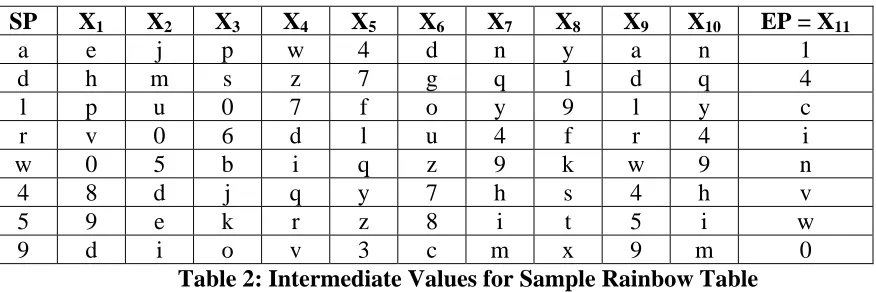
[image:38.612.90.528.309.455.2]

random starting points must be selected. The starting point must be encrypted, have the reduction function applied, and converted back to plaintext to get each intermediate point. There exist t intermediate points. The final intermediate point is commonly referred to as the endpoint. Only the starting point and the endpoint are stored in memory. The data table on the following page provides eight randomly selected starting points, all chain intermediate points, and the ending point for each chain.

SP X1 X2 X3 X4 X5 X6 X7 X8 X9 X10 EP = X11

a e j p w 4 d n y a n 1

d h m s z 7 g q 1 d q 4

l p u 0 7 f o y 9 l y c

r v 0 6 d l u 4 f r 4 i

w 0 5 b i q z 9 k w 9 n

4 8 d j q y 7 h s 4 h v

5 9 e k r z 8 i t 5 i w

9 d i o v 3 c m x 9 m 0

Table 2: Intermediate Values for Sample Rainbow Table

Recall that each plaintext value in the column labeled “SP” has been randomly selected from the plaintext space of a-z and 0-9 with a length of 1. Again, this example is simplified and the plaintext strings could be longer than 1, but for this example, only a single character is being encrypted. To generate the value of the first chain column labeled X1, the starting point must be encrypted, have the reduction function applied, and then mapped back to the plaintext space.

(39)

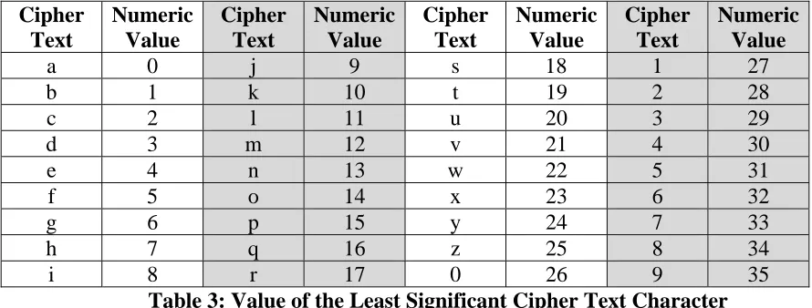
found. If the plaintext space is numbered from 0 – 35, the letter ‘a’ would be valued at 0, ‘b’ would be valued at 1, ‘c’ would be valued at 2, the letter ‘d’ would be valued at 3, etc. The values of the least significant Cipher Text character can be seen in Table 3.

Cipher Text

Numeric Value

Cipher Text

Cipher Text

a 0 j 9 s 18 1 27

b 1 k 10 t 19 2 28

c 2 l 11 u 20 3 29

d 3 m 12 v 21 4 30

e 4 n 13 w 22 5 31

f 5 o 14 x 23 6 32

g 6 p 15 y 24 7 33

h 7 q 16 z 25 8 34

[image:39.612.84.529.182.351.2]

i 8 r 17 0 26 9 35

Table 3: Value of the Least Significant Cipher Text Character

The next most significant character in the cipher text is the letter ‘a’. As seen in Table 4, the value of ‘a’ is also zero when it appears in the most significant position. Adding the values of the least and most significant positions of the cipher text provides us with a numeric equivalent of that cipher text. Thus, the cipher text of ‘ad’ maps to the numeric equivalent value of 4.

(40)

Cipher Text

Cipher Text

a 0 j 324 s 648 1 972

b 36 k 360 t 684 2 1,008

c 72 l 396 u 720 3 1,044

d 108 m 432 v 756 4 1,080

e 144 n 468 w 792 5 1,116

f 180 o 504 x 828 6 1,152

g 216 p 540 y 864 7 1,188

h 252 q 576 z 900 8 1,224

i 288 r 612 0 936 9 1,260

Table 4: Value of the Most Significant Cipher Text Character

Examining the starting point of ‘9’ from Table 1, it is known that the cipher text is ‘9c’. From Table 3 and Table 4, we find that the character ‘c’ for the least significant position is valued at 2 and the character ‘9’ in the most significant position is valued at 1,260. Adding them together, we get 1,262. This is the numeric value of the cipher text of ‘9c’.

Once this numeric value is determined, it must be mapped back onto the plaintext. This mapping is implemented by applying the reduction function. Per section 3.4.2, the reduction function we are using is quite simplistic. To apply the reduction function, add the column position to the numeric value of the cipher text, and then use the modulo function with a divisor of the size of the plaintext space, which in this case is 36. This guarantees that the resulting value will be between 0-35, so as to provide a direct mapping to a new plaintext value. Table 5, Table 6, Table 7, and Table 8 show the

(41)

SP

Cipher

Text

Cipher

Text

Value R0 X1

Cipher

Text

Cipher

Text

Value R1 X2

Cipher

Text

Cipher

Text

Value R2 X3

a ad 3 4 e eh 151 9 j jm 336 15 p

d dg 114 7 h hk 262 12 m mp 447 18 s l lo 410 15 p ps 558 20 u ux 743 26 0 r ru 632 21 v vy 780 26 0 03 965 32 6

w wz 817 26 0 03 965 31 5 58 1,150 1 b

4 47 1,113 34 8 8b 1,225 3 d dg 114 9 j

5 58 1,150 35 9 9c 1,262 4 e eh 151 10 k

9 9c 1,298 3 d dg 114 8 i il 299 14 o

Table 5: Starting Point through Chain Position X3

Now look at a specific example for generating chains in the rainbow table. For the starting point ‘a’, the cipher text value is ‘ad’, and the numeric value for that cipher text is 3. Add 1 to the value of 3 (because this is the first ‘column’ in the chain) and apply the modulo function. This shows that 4 mod 36 = 4. Looking up the plaintext from Table 3 of the value 4, it is found to be the plaintext character ‘e’. This is the first chain position, which is labeled X1.

Next, the plaintext at X1 is encrypted and becomes ‘eh’. Per the previous tables, this cipher text as a numeric value is found to be 151. Now add 2 to that number (because this is the second ‘column’ and the reduction function for the second column must be applied) prior to performing the modulo arithmetic. Thus, we have 153 modulo 36 = 9.

(42)

X3

Cipher

Text

Cipher

Text

Value R3 X4

Cipher

Text

Cipher

Text

Value R4 X5

Cipher

Text

Cipher

Text

Value R5 X6

p ps 558 22 w wz 817 30 4 47 1,113 3 d

s sv 669 25 z z2 928 33 7 7a 1,188 6 g

0 03 965 33 7 7a 1,188 5 f fi 188 14 o

6 69 1,187 3 d dg 114 11 l lo 410 20 u

b be 40 8 i il 299 16 q qt 595 25 z

j jm 336 16 q qt 595 24 y y1 891 33 7

k kn 373 17 r ru 632 25 z z2 928 34 8

o or 521 21 v vy 780 29 3 36 1,076 2 c

Table 6: Chain Position X3 through Chain Position X6

X6

Cipher

Text

Cipher

Text

Value R6 X7

Cipher

Text

Cipher

Text

Value R7 X8

Cipher

Text

Cipher

Text

Value R8 X9

d dg 114 13 n nq 484 24 y y1 891 0 a

g gj 225 16 q qt 595 27 1 14 1,002 3 d

o or 521 24 y y1 891 35 9 9c 1,262 11 l

u ux 743 30 4 47 1,113 5 f fi 188 17 r

z z2 928 35 9 9c 1,262 10 k kn 373 22 w

7 7a 1,188 7 h hk 262 18 s sv 669 30 4

8 8b 1,225 8 i il 299 19 t tw 706 31 5

c cf 77 12 m mp 447 23 x x0 854 35 9

Table 7: Chain Position X6 through Chain Position X9

X9

Cipher

Text

Cipher

Text

Value R9 X10

Cipher

Text

Cipher

Text

Value R10 EP = X11

a ad 3 13 n nq 484 27 1

d dg 114 16 q qt 595 30 4

l lo 410 24 y y1 891 2 c

r ru 632 30 4 47 1,113 8 i

w wz 817 35 9 9c 1,262 13 n

4 47 1,113 7 h hk 262 21 v

5 58 1,150 8 i il 299 22 w

9 9c 1,262 12 m mp 447 26 0

(43)

3.4.5 Using a Rainbow Table for Decryption

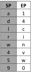
Typically, the resulting rainbow table would be sorted by the endpoint, so as to allow fast binary searching. This optimization shall be ignored in this example. The final rainbow table in this example is shown in Table 9. Note that to store this rainbow table requires only 2 bytes of storage per chain for a total of 16 bytes. To store an entire lookup table for the entire plaintext space would require 3 bytes for every plaintext value, thus would require 108 bytes total. Note that the rainbow table is less than one-sixth of the size requirement for storing the full table, thus the space savings are considerable.

SP EP

a 1

d 4

l c

r i

w n

4 v

5 w

[image:43.612.275.339.296.439.2]

9 0

Table 9: Final Example Rainbow Table

To use a rainbow table for decrypting information, the underlying assumption is that we have access to the encrypted data. Assume that the encrypted data we have been provided with is ‘hk’. The first step in decrypting the data is to see if this matches with any of the endpoints by applying the reduction function Rn-1 where n is a counter that begins with a value of the chain length.

(44)

Since a match has been identified, the corresponding starting point for the chain is identified as the plaintext of ‘4’. To find the plaintext for which ‘hk’ is the cipher text, start at the plaintext of ‘4’, then encipher, map, and reduce the plaintext for n - 1 times. Thus, we apply this sequence of instructions 10 times’.

From Table 8, we see that the plaintext at X10 is ‘h’. This is considered to be a potential match. If encrypting the plaintext of ‘h’ results in ‘hk’, then the plaintext has been found and the hash has been decrypted. If encrypting the plaintext found at this position in the chain results in anything other than ‘hk’, then a false positive has been encountered. False positives can occur due to the reduction function that maps a larger set of encrypted values back onto a smaller set of plaintext values. This can cause multiple hashes to map back to the same plaintext, which in turn can cause false positives.

If applying the reduction function Rn-1 to the cipher text does not yield a match to an endpoint, the result is thrown away and Rn-2 is applied instead. If a potential match is found, then the process of enciphering, mapping, and reducing the plaintext is applied

n - 2 times. If this does not yield a matching result, then the reduction function Rn-3 is applied. This continues until all reduction functions have been applied or a valid plaintext match has been found.

3.5. Summary

(45)

The single biggest problem with any of these methods is the sheer time required to pre-compute the lookup tables. Neglecting disk write times, a reasonably fast computer can achieve a hashing rate of 2 million md5 hashes per second. The examples provided in the introduction of this chapter would take approximately 16 days and 38,733 days, respectively. While the first timeframe is tolerable, the second is not.

(46)

Chapter 4

Parallel analysis and design

Parallel computing is a methodology used to decrease the amount of time required to solve a large problem by dividing it into smaller tasks which are solved concurrently. This parallelism can be achieved using either hardware, software, or a combination of the two.

This chapter focuses on analyzing how to address the parallelization of rainbow table generation from the software perspective. First, an introduction to parallel computing is provided. Next in Chapter 4.2 task granularity is explored, followed by an analysis of rainbow table task granularity in Chapter 4.3. In Chapters 4.4 – 4.6, the effect of hardware resources on task granularity is detailed for the md5 algorithm on the test hardware being used.

In Chapter 4.7, the resulting software architecture is described, including the rationale for various design choices, such as network latencies, processor speeds, and work assignment. Finally, Chapter 4.8 summarizes the analysis and design.

4.1. Introduction to Parallel Computing

Amdahl’s Law [14] states that the potential speedup of any application when moved from a single processor to multiple processors is governed by the following equation, where P is the fraction of the application that is parallelizable and N is the number of processors used.

1

(47)

Any sufficiently large problem will consist of parts that are parallelizable and parts that must be evaluated sequentially. For example, in all of the time-memory tradeoff algorithms discussed in this thesis, building of an individual chain is considered to be a sequential procedure that may not be parallelized, due to the inherent dependencies upon previous results in the chain.

As N approaches infinity, the maximum speedup factor that can be achieved is:

1

Amdahl forwards this theory based on a fixed problem size that has been misused over the years to argue against parallelization. In essence, Amdahl’s law states that if a problem has a serial component that accounts for 10% of the application runtime, then we can achieve no more than a 10x speedup. For more than 30 years, this was used to argue against parallel computing because it could not be refuted.

While Amdahl’s Law is still regarded as being technically accurate, Gustafson formulated a new method [15] of calculating the speedup and expanded the apparent usefulness of parallel computing. Gustafson points out that Amdahl’s Law is only directly applicable when the problem is a fixed size, thus the problem has already been explored in an entirely measurable sequential manner.

(48)

Let n represent the size of the problem. Let the function a represent the sequential fraction of the application and the function b represent the parallel fraction of the application. Thus:

1

To generalize the time equation, we have:

1

where p represents the number of processors. The speedup achieved by increasing the problem size is thus:

1

Research done by Yuan Shi [16] in 1996 shows that Amdahl’s Law is mathematically equivalent to Gustafson’s Law. He points out that there are several prerequisites to applying Amdahl’s Law and that they are often neglected. The primary prerequisite to the application of the law is that “the serial and parallel programs must compute the same total number of steps for the same input”. He suggests that only time-based formulations should be used for evaluating the performance of parallel applications.

(49)

but the work associated with doing so is only going to be applicable to a specific problem and may not be generalized.

4.2. Parallel

Granularity

In parallel computing, granularity is a relative measurement of the ratio of computation to communication. This often results in classifying something as either a course grained task or a fine grained task. Course grained tasks tend to have very little communication, while fine grained tasks tend to be more communications intensive. The classification can be applied to discrete portions of the application, or to the application as a whole. It is not uncommon to have a course grained parallel application with some fine grained components.

A third measure of granularity is not often used, but does exist. It is called “embarrassingly parallel” and refers to any tasks which exhibit massively inherent parallelism. An embarrassingly parallel task is any task for which the problem size can be scaled up dramatically to N processors, and achieve a speedup of approximately N, due to the lack of communications required between tasks.

(50)

Analyzing the granularity of a problem is an important part of determining how easily the solution can be parallelized and can provide a good approximation of what the anticipated speedup would be. Based on a machine size that is measured in the number of processors, the optimal granularity can change [17]. Hammond, Loidl and Partridge described a tool for analyzing task granularity and attempting to quantify the optimal grain size for parallel applications.

The inherent difficulty in quantifying the optimal grain size has led to studies that assist programmers in visualizing communication patterns [18]. However, additional research [19] illustrates that simply identifying the communication patterns between objects in memory and using those objects as independent tasks is not enough for two important reasons. The first relates to the fact that creating new objects in memory in a serial application is done many times per second, yet is necessary to do so. While the performance costs of doing so tends to be high, the costs become prohibitive in a parallel environment due to additional overhead.

The second reason is that communication costs become prohibitive when every object in memory becomes a separate task and thus is required to communicate separately with every other task. It makes no difference whether the messages are sent using shared memory, or some sort of message passing library. The sheer number of additional data objects in memory that must be created and the overhead incurred by either shared memory or network library messages makes this prohibitive. Even shared memory

(51)

4.3. Granularity of Rainbow Table Generation Tasks

The generation of rainbow tables is an inherently massively parallel operation. Virtually no communication is required between the processors that are generating the chains. In theory, the speedup that can be achieved by parallelizing the table generation can be as high as the number of chains, where each processor is assigned a single chain to generate from a data table. This neglects the time required to combine the results. Of course, housing each result on a separate processor would result in the capability to perform a massively parallel decryption effort.

It is not particularly realistic to use a separate processor for every chain, as a single rainbow table may consist of over a hundred million chains and the network transmission costs associated with assigning extremely tiny workloads would greatly hinder the performance of the system. Instead, number of chains must be divided such that they may be assigned to different processors in the system with the goal being that all processors finish their work at approximately the same time. In a cluster configuration or any homogeneous environment, this is a very straightforward task and falls under the category of “embarrassingly parallel”.

(52)

hardware environments as opposed to homogeneous hardware. This has a direct impact on the granularity of the tasks that can be assigned.

In a homogeneous environment, the task size would likely be , where N is the

number of processors and mt is the total number of hashes to be produced. In a heterogeneous environment, this is no longer the most efficient division of tasks. The efficiency of the system can be modeled by the following equation:

1

For every processor in the system, we sum the idle time percentage and divide by the total number of processors. The resulting percentage is subtracted from 1 to give us our final efficiency, which is the amount of time that processors in the system are idle in relation to the time that they are doing work.

Take, for example, a system with five processors, four of which are 0% idle and the fifth is 50% idle. This results in an Efficiency of the system of:

1 0

5 0 5

0 5

0.5

5 90%

Intuitively, this makes sense because each processor is expected to do about 20% of the work and four are 100% busy, resulting in 80% efficiency. The fifth processor is only working half the time, thus only contributing half of its available CPU cycles to the task at hand doing meaningful work, thus the addition of an additional 10% efficiency for a total of 90%.

(53)

processor were fully loaded throughout the life of the parallel program, then efficiency would be 100%. In practice, this would not be likely. To divide the work in a meaningful way that is more efficient, we need to account for differences in disk I/O, processor hashing speeds, fluctuating workloads, and network messaging overhead.

4.4. Disk I/O Considerations

The number of disk accesses is relative, from one processor to another. The faster a processor is able to process units of work, the more disk accesses it will do. The proportion of disk accesses will grow in direct proportion to the speed at which an individual processor completes chains, as the starting and ending points of a chain are written to disk at the same time immediately after the ending point has been calculated.

(54)

Computer Specifications Approximate MD5 hashing speed (hashes/second per processing unit)

Approximate Total hashing speed across all processors

1) Quad Core E5405 2.0GHz Xeon 4.0 GB RAM

10,000 RPM SCSI hard disk

1,183,000 hashes/second

4,732,000 hashes/second 2) Dual Core Athlon XP 2.6GHz

3.0 GB RAM

7,200 RPM SATA hard disk

2,623,000 hashes/second

5,246,000 hashes/second 3) Dual processor 2.4GHz Xeon

2.0 GB of RAM

10,000 RPM SCSI hard disk

695,000 hashes/second 1,390,000 hashes/second

Table 10: Sample test machine hashing speeds

Based on the approximate hashing speeds seen in Table 10, we can calculate approximately how much data will be written to the hard disk each second of processing. The amount of data written is a function of the chain length and is illustrated by both the following equation and the following chart.

(55)

Chart 1: Bytes/second vs. Chain Length

The number of bytes per second written to disk is quite small, as indicated by the above graph. The maximum bytes/second being written to disk is no more than 9,000 in a worst case scenario, which is on Computer #2. We must consider that the worst case scenario on this computer is that both processors are writing to the disk at the same time, thus generating 18,000 bytes/second of disk I/O. The hard disk for this computer is rated at a theoretical 3Gbps, thus providing 402,653,184 bytes/second of bandwidth. The actual disk I/O is a tiny fraction of the I/O that the disk is capable of.

One might also consider that the number of disk accesses per second could influence the results. During testing on Computer #1, it was found that decreasing the chain length to 1 and generating 10 million chains resulted in approximately 156 MB of data written to disk. The anticipated time for completion was only 7.1 seconds, but the measured speed was approximately 21 seconds. The available bandwidth to disk would

0 1000 2000 3000 4000 5000 6000 7000 8000 9000

2,500 5,000 10,000 25,000 50,000 100,000

Bytes/Second

to

disk

Chain Length

(56)

indicate that the system can write 156 MB of data to disk in less than 2 seconds, which does not account for the additional 14 seconds of processing time.

A second test using a chain length of 1,000 and 10,000 chains requires a total of 10 million hashes, just as the first test does. In this test, the calculated optimal time was between 7.15 – 7.18 seconds and the measured time was 7.17 seconds. These tests show that disk accesses per second can play an important role in table generation speed.

In practice, disk access has minimal impact on the application because chain lengths are typically in the thousands, or tens of thousands. When chain lengths of more than 1,000 are used, there are significantly fewer disk accesses per second. Modern disk caching techniques tend to reduce or eliminate delays associated with writing data to disk in 8 byte blocks. A common programming technique that takes advantage of head location on the disk is to cache many values to memory and write a single large block of data all at once. This is especially useful for older hard disks or ones that do not support command queuing architecture. Chain lengths of less than 1,000 are not practical in any case.

4.5. Differences in Processor Hashing Speeds

(57)

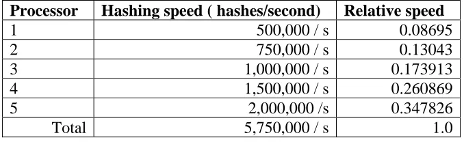
ago. Finally, Computer #3 is using much older processors which are approximately 6-7 years old. Table 11 outlines the differences between these processors.

Computer Hash speed/processor

CPU Speed

Bus Speed L2 Cache size

1) Intel E5405 1,183,000 / s 2.0 GHz 1333 MHz 2 x 6MB 2) Athlon XP 5200+ 2,623,000 / s 2.6 GHz 2 x 1 GHz 2 x 1024KB 3) Intel Xeon 2.4GHz 695,000 / s 2.4 GHz 533 MHz 512 KB

Table 11: Processor Comparison

It is to be expected that Computer #3 is measurably slower, primarily due to the age of the computer architecture. The processors are located in separate sockets which reduce potential issues with shared cache, but the processors only have 512KB of L2 cache, and the Bus Speed is only 533MHz.

More interesting than Computer #3 is the comparison between Computer #1 and Computer #2. The hashing speed of Computer #2 is more than twice that of Computer #1. A variety of hardware differences could help to explain this, however as we pointed out previously, disk I/O is minimal so it really comes down to system memory, CPU speed, bus speed, cache size, and computer architecture.

(58)

have a great enough effect on the computer to account for a doubling or halving of the hashing speed.

The CPU speed is the most likely culprit that influences hashing speed. Computer #3 has a 20% greater raw CPU speed than Computer #1, yet benchmarks at only half the hashing speed of Computer #1. Computer #2 is 30% faster than Computer #1 in this regard, yet benchmarks at more than double Computer #1. CPU speed alone does not seem to be the most significant factor in the hashing speed, but it must be a contributing factor.

Bus speed, cache size and computer architecture are the only remaining factors. The significantly lower bus speed of Computer #3 would seem to account for the difference in hashing speed between Computer #3 and the other computers. However, the bus speed differences between Computer #1 and Computer #2 must be evaluated further. The cache is structured differently between the two types of processors so we must eliminate that first.

The Intel processor shares 6MB of L2 cache between 2 processors while the AMD processor provides 1MB of cache to each processor. It is possible that cache thrashing might be responsible for reduced hashing speeds, but a simple test using only one of the 4 CPU’s on the Intel processor eliminated this as a possibility, thus the cache sharing does not impact the hashing speed, and because the Intel processor has more cache to begin with, this cannot be a factor.

(59)

processor architectures are such that the bus speed is not a direct comparison. The Intel processor shares the bus across all four processors, while the AMD processor has a separate bus for each processor, each running at the same speed.

We can theorize that if the processor bus were shared across all four Intel processors, then the theoretical speed of the bus might be only 333MHz. Testing has shown that whether we use only one CPU on this processor or four at the same time, the hashing speed is not affected so this theory is not plausible. The bus speed of the Intel processor seems to be faster than that of the AMD Athlon processor.

The preceding information leads to only one possible conclusion. The processor architecture is the single most significant factor in hashing speed. While various other differences between the processors may be contributing factors, none can individually or collectively account for the significant differences in hashing speed from one processor to another more than the processor architecture.

4.6. Network

Topology

Fundamentally, the network is the slowest component of the average computer. This statement holds true even with the introduction of gigabit Ethernet. High speed clusters may be built that use fiber optic network devices which dramatically reduce the network access times and transmission latencies between nodes of a system to less than that of disk access. These clusters are not in easy reach of the average user, and thus not the focus of this thesis.

(60)

There are numerous types of distributed-memory MIMD systems which are broadly categorized by their network connections into either static or dynamic networks. Static networks are those where the nodes are directly connected to one another, in whatever configuration has been deemed appropriate. In a dynamic network, some nodes are connected to switches, which dynamically determine where to route traffic based on routing information provided with the network traffic.

Modern