Exploration of the effect of surface roughness on heat transfer in microscale liquid flow

(1)

Theses Thesis/Dissertation Collections

2010

Exploration of the effect of surface roughness on

heat transfer in microscale liquid flow

Nicholas M. Schneider

Follow this and additional works at:http://scholarworks.rit.edu/theses

This Thesis is brought to you for free and open access by the Thesis/Dissertation Collections at RIT Scholar Works. It has been accepted for inclusion

in Theses by an authorized administrator of RIT Scholar Works. For more information, please [email protected].

Recommended Citation

(2)

HEAT

TRANSFER IN

MICROSCALE

LIQUID

FLOW

by

A Thesis Submitted in Partial Fulfillment of the Requirements for a B.S./M.S. in

Mechanical Engineering

Thesis Advisor:

Dr. Satish G. Kandlikar Professor of Mechanical Engineering

Approved by:

Dr. Steven J. Weinstein

Professor and Department Head of Chemical and Biomedical Engineering

Approved by:

Dr. David J. Gee Assistant Professor of Mechanical Engineering

Approved by:

Dr. Ting-Yu Lin

Postdoctoral Research Associate, Department of Mechanical Engineering

Approved by:

(3)

Rochester Institute of Technology

Kate Gleason College of Engineering

Title:

Exploration of the Effect of Surface Roughness on Heat Transfer in

Microscale Liquid Flow

I, Nicholas M. Schneider, hereby grant permission to the Wallace Memorial Library

of the Rochester Institute of Technology to reproduce my thesis in whole or part. Any

reproduction will not be for commercial use or profit.

(4)

Abstract

Exploration of the Effect of Surface Roughness on Heat Transfer in

Microscale Liquid Flow

Thesis Advisor: Dr. Satish G. Kandlikar

As technology provides smaller devices with greater heat dissipation needs,

microflu-dic systems become essential. The scale of device architecture causes concerns to arise

that were previously not an issue. The results of manufacturing processes, such as

rough-ness structures on machined surfaces, now play a significant role in transport phenomena.

This study takes an analytical and experimental approach to understanding the

fundamen-tal heat transfer process in rectangular channels with artificially roughened walls. Steady,

incompressible, fully developed liquid flow is modeled with lubrication theory to develop

an expression for the fully developed Nusselt number. The heat transfer performance of the

small aspect ratio rectangular channels with two wall heating under the H2 boundary

con-dition is experimentally investigated. A constant wall heat flux is applied at opposing long

walls. Four different structured roughness geometries are investigated along with smooth

channels as the heated walls. In total, hydraulic diameters ranged from Dh = 183µmto

Dh = 1698µmand were tested over a Reynolds number range of45to600. The pitch to

height ratio of the sinusoidal roughness surfaces covered the ranged of 2.6to 10.6. The

resulting relative roughness was2.17%to16.53%. Fully developed Nusselt was found to

lie below classic theory. Sinusoidal roughness geometries were found not to provide heat

(5)

List of Figures

1.1 Reproduction of results from Wu and Cheng [2] . . . 5

1.2 Roughness Visualization . . . 10

1.3 Constricted Parameter Performance . . . 12

2.1 Smooth Channel Domain Illustration . . . 16

2.2 Wavy Wall Domain Illustration . . . 19

3.1 Axial Conduction,M Comparison of Aluminum and Stainless Steel . . . . 26

3.2 Axial Conduction,M for Stainless Steel . . . 26

3.3 Test Piece Ground Surfaces . . . 27

3.4 Test Section Assmebly . . . 28

3.5 Test Piece Example . . . 29

3.6 Gauge Block Illustration . . . 29

3.7 Base Block Design . . . 30

3.8 System Architecture . . . 32

3.9 36AWG Thermocouple Weld . . . 34

3.10 LABVIEWTMGUI . . . 34

3.11 Structured Roughness Design Parameters . . . 35

3.12 Test Setup Assembly . . . 36

3.13 Test Setup Assembly . . . 37

3.14 Pressure Sensor Calibration Curve . . . 38

3.15 Flow Meter Calibration Curve . . . 39

3.16 Heat Loss Curve . . . 41

3.17 Experimental Friction Factor Compared to Conventional Theory . . . 42

4.1 Laser Confocal Surface Results . . . 44

4.2 Curve Fit Coefficients . . . 45

4.3 Surface Rendering ofλ/h= 2.6 . . . 46

(8)

4.7 Channel Orientation . . . 49

6.1 Channel Orientation . . . 59

6.2 Smooth wall results as a function ofRe . . . 60

6.3 Smooth wall results as a function ofαRe . . . 61

6.4 N u∗ vsReforλ/h= 4.8Sinusoidal Roughness . . . 63

6.5 N u∗ vsαReforλ/h= 4.8Sinusoidal Roughness . . . 65

6.6 N u∗ vsαReforλ/h= 4.8Sinusoidal Roughness,AactualCompared toAP 66 6.7 N u∗ vsαRefor All Sinusoidal Roughness . . . 67

6.8 N u∗ overε/D . . . 68

6.9 Local Nusselt Number ( Smooth,Dh = 1698µm,Re= 105) . . . 69

6.10 Local Nusselt Number (λ/h= 4.8,Dh = 1115µm,Re= 65) . . . 70

6.11 Reproduction of results from Hetsroniet al.[34] . . . 72

6.12 Reproduction of results from Quet al.[19] . . . 73

(9)

Nomenclature

Symbols

A- Area

a- Channel height

b- Root Channel Separation

Cp- Specific Heat Capacity

Dh- Hydraulic Diameter

F dRa- Floor Distance to Mean Line

f - Friction Factor

h- Roughness Height

¯

h- Heat Transfer Coefficient

k- Thermal Conductivity

L- Length

M - Axial Conduction Number, Eqn. (1.2)

˙

m- Mass Flow Rate

N u- Nusselt Number

P - Pressure

P r- Prandtl Number

Q- Power

q- Heat Flux

Ra- Average Roughness Height

Rp - Maximum Peak Height

RSM - Mean Spacing Between Peaks

Rv - Lowest Valley

Re- Reynolds Number

T - Temperature

u-xˆComponent of Velocity

~

V - Velocity Vector

˙

V - Volumetric Flow Rate

v -yˆComponent of Velocity

< v >- Average Velocity

xf d - Thermal Developing Length

α- aspect ratio (α =b/a)

αf - Thermal Diffusivity

ε- Average Roughness Height

ρ- Density

Subscripts

actual- Actual Surface Based on Arclength

ave- Average

cf - Constricted Parameter

cond- Conduction

conv - Convection

f - Fluid

H - Heater

i- ith Thermocouple

L- Local

P - Projected Surface

room- Ambient

s- solid

(10)

Chapter 1

Introduction

Microfluidic devices are becoming necessary in diverse fields and new technologies.

Un-derstanding the underlying fundamental physics of the transport phenomena occurring in

devices whose scale is continuously decreasing in size is essential for optimal design. The

ratio of surface area to volume in small channels provides characteristics exploitable in heat

transfer applications. In the specific application of electronics chip cooling, it is desirable

to maximize heat dissipation with minimal energy input.

Laminar forced convection in single phase flow is appealing due to the lower pressure

drop associated with this regime. Modifications in channel wall geometry have shown

potential to increase heat transfer in ducts with minimal pressure drop costs. However, due

to experimental uncertainties, the complexity of the coupled physics problem, and the lack

of an in-depth systematic study researchers are left inconclusive and contradictory results.

The aim of this study is to develop and test an experiment design which isolates sources of

uncertainty and identifies the key parameters necessary for accurate experimental results,

while fully investigating the controlled geometry of sinusoidal wall roughness.

1.1

Literature Review

1.1.1

Surface Roughness and Heat Transfer

The effect of surface roughness on low Reynolds number flow is receiving substantial

(11)

including PEM fuel cells and electronics, requiring high heat flux removal are providing

new avenues for the use of mini- and microchannels [1,2,3,4-11]. In current literature, the

effects of surface roughness are still ambiguous due to the compounding effects of the

de-veloping entrance region, early transition to turbulence, and high experimental uncertainty.

This study will mitigate these issues by using designed structure roughness to better control

the overall system.

Most research regarding surface roughness effects on heat transfer has been performed

at macroscale. Gao and Sunden [12] studied air flow through rectangular ducts with

hy-draulic diameters of 24.9 mmand700 mm. Reynolds number was varied between 1000

and 6000 to examine the temperature distribution across a rib with surface roughness. The

data collected was used to find the local and average heat transfer coefficients along with

the Nusselt numbers. The ribs were found to enhance the heat transfer process compared to

smooth ducts. Friction factors for different rib orientations were also investigated in their

study. The authors found the greatest heat transfer to occur at the tips of the rib roughness

elements, with the lowest heat transfer occurring at the base of the ribs.

Changet al. [13] recently investigated the effects of scale shaped roughness elements on the heat transfer characteristics of air flow through rectangular channels. A large range

for Reynolds number was chosen to cover the range from 1500 to 15000. The authors

used various roughness element configurations for the study, and concluded that the scaled

roughness elements enhanced heat transfer with better performance than rib shaped

rough-ness elements.

In 1994 Ling et al. studied how triangular shaped rib-roughness in channels effected the heat and mass transfer [14]. The paper lacks the details on channel dimensions and the

means of heating. The authors chose Reynolds numbers to correspond with the turbulent

regime. Reynolds number was varied from 10,000 to 70,000 over systematically placed rib

(12)

Entrance length was found to increase with Reynolds number. Heat and mass transfer rates

were increased by a factor of up to 2.3 over the smooth channel equivalent. The increase

of heat and mass transfer was also found to a function of Reynolds number, while friction

factor,f, was a weak function of Reynolds number.

Heat transfer characteristics of water in stainless steal minitubes with inner diameters

of 1067and 620 µmwere studied by Kandlikar et al. [3]. The experiments utilized two different etches in order to create a variety of surface roughness inside the minitubes. The

average roughness of the tubes ranged from 1 µm to 3 µm, corresponding to a relative

roughness range of0.161%to0.355%. The study was focused on the laminar flow regime,

and was determined to have thermally developing conditions. With consideration to the

conditions, the experimental data was compared with correlations available at the time. For

the smoothest tubes and all of the roughness ranges of the1067µmtube, the experimental

data was found to correspond to the predicted values within uncertainties. The smaller

tube, the620µmtube, was under-predicted by the correlation as roughness increased. This

deviation lead the authors to conclude that more research is necessary to understand the

effects of surface roughness as the diameter becomes smaller.

Bucci et al. in 2003 investigated fluid flow and heat transfer properties in capillary tubes [8]. Hydraulic diameters of 172 µm, 290 µm, and 520µm were selected and

sub-ject to both laminar and turbulent flows, with Reynolds number ranging from 100 to 6000.

Roughness was reported as an absolute height ranging from 1.498 µm to2.166 µm, the

authors used a laser interferometric microscope to obtain the roughness values. The

out-side wall temperature was held constant via water vapor condensation. The results fit the

Gnielinski correlation well for the two larger diameter tubes in the turbulent regime. The

two smaller diameter tubes did not fit the Gnielinski correlation well for turbulent flow.

The Hausen correlation under-predicted the experimental data from the laminar regime.

(13)

The investigation considered Reynolds numbers from10,000to90,000in four tubes with

diameters of1931µm, 1042µm, 834µm, and531µm. The objective was to understand

the effects of surface roughness on single-phase pressure drop and heat transfer

proper-ties in the four given stainless steal minitubes. The experimental Nusselt number results

were under-predicted by the Dittus-Boelter and Gnielinski correlations for their respective

ranges. The authors also noted that the discrepancies increased as channel diameter

de-creased. Overall, surface roughness was found to improve heat transfer properties in the

minitubes.

Hegab et al. in 2001 studied rectangular microchannels with R-134a refrigerant [16]. The goal was to understand the effects of channel geometry and Reynolds number on

con-vective heat transfer. Hydraulic diameter was chosen to range from112µmto210µmwith

varying aspect ratios from 1to 1.5. In order to mitigate error, the authors paid particular

attention to measurements. The surface profile was measured with a profilometer to more

accurately know the roughness of the test pieces. A microscope and video camera were

em-ployed to measure the channel width, while digital dial calipers were used to measure the

length. Reynolds number ranged from2000to4000in the experiments. This range, being

the transition range, allowed the results for the Nusselt number to be compared to

Gnielin-ski’s correlation. Wall temperatures were calculated by means of a conduction heat transfer

analysis utilizing the average temperature measured by seven thermocouples located on the

back of the wafer. The authors found that both the friction factor and the Nusselt number

were over-predicted by conventional correlations ranging from6%to84%. The deviations

were found to decrease as channel diameter increase or Reynolds number decreased.

Lee et al. in 2005 investigated single-phase heat transfer in rectangular minichannels

[17]. The corresponding hydraulic diameters ranged from318 µmto 903 µm. Reynolds

number was varied from 300 to 3500 for five channel configurations. The experimental

(14)

developed flows. Deviation from classic theory was inversely related to channel size for a

given flow rate.

Wu and Cheng in 2003 studied laminar water flow through trapezoidal silicon mini- and

microchannels [2]. The experimental variables were: geometry, hydrophilic properties, and

surface roughness. These properties were varied over thirteen channels etched in a silicon

wafer. Ten out of the thirteen channels had silicon for the surface material, and the other

three had a thermal oxide layer deposited to increase the surface hydrophilic properties.

The first set of channels also had geometry and relative roughness variances to see the

effects of all the chosen variables. Different etching processes were used to vary the relative

roughness of the channels. The wafer was heated by a thin film heater attached to a DC

power supply. Reynolds number was varied up to 1500, and the effects on heat and mass

flow were observed. Their results for Nusselt number as a function of Reynolds number

can be seen in the reproduction found in Figure 1.1.

1 1.5 2 2.5

N

u

0 0.5

0 100 200 300 400 500 600 700

Re

Dh = 82um

[image:14.612.174.464.428.646.2]

Dh = 84um

(15)

A few experimental studies have found that fluid flow in smooth microchannels does

not deviate from conventional theory. Yang and Lin [18] examined water flow through

six stainless steal mini and microtubes with diameters ranging from 123 µm to962 µm.

Reynolds number was varied through both the laminar and turbulent regimes with values

up to 10,000 being studied. The surface temperature of the tubes was acquired by means

of Liquid Crystal Thermography. The tubes were heated by DC powered heaters clamped

to each end of the tubes. The average roughness for the tubes ranged from1.16µmto1.48

µm. The experimental results for the laminar flow Nusselt number were found to agree

well with the theoretical values for fully developed flow with constant heat flux. Turbulent

results were compared with the Gnielinski correlation, and were also found to fit well.

Finally, the developing region Nusselt number was also found to agree with the Shah and

Bhatti correlations. The authors concluded that there is no deviation from classic theory

for the range of diameters investigated in their study.

Given discrepancies in current literature, more research on the effects of surface

rough-ness on heat and mass transfer is necessary to develop a model that will accurately predict

these effects. It is important to better understand these transport phenomena while paying

close attention to uncertainty generated in test results. It is also important to define at what

point roughness becomes a non-negligible issue for microfluidic scenarios. This work will

aim to generate a theoretical model that fulfills the fore-given requirements.

1.1.2

Axial Conduction

Axial heat conduction in channel walls is generally low in conventional sized channels

where the channel diameter is greater than3mm. The axial conduction effects are small

because the channel walls are relatively thin compared to the overall channel size and flow

length. In mini and microchannels, the convective heat transfer becomes significantly

ef-fected due to the relatively large multi-dimensional conduction in the wall. A number of

(16)

the channel without considering the multidimensional conduction in the wall [2, 19, 20,

21]. These studies showed that the heat transfer coefficient was smaller for microscale

compared to conventional macroscale results. Guo and Li indicated that it might be due

to the error introduced by the assumption of one-dimensional heat conduction in the wall

[22]. The results show that without considering the axial heat conduction in the walls, the

experimental Nusselt number will be lower than the actual value. Chiou [23] presented a

conductance number,cond, to describe the effects of axial heat conduction in the walls on

convective heat transfer.

cond= ksAs

Lm˙fcp,f

=

As

Af

L D

1

ReP r ks

kf

(1.1)

whereks,As,kf, andAf are the thermal conductivity and cross-sectional area for the tube

wall and fluid. The other parameters: L,D,m˙f, andcp,f are the tube length, tube diameter,

mass flow rate of the fluid, and the specific heat of the fluid respectively. Forcondless than

0.005, the effects of axial heat conduction are negligible. A non-dimensional number,M,

was proposed by Maranzanaet al. [24] to quantify the role of axial conduction in the walls.

M = qcond

qconv

= ks

esw

L

ρcp,fefwV

(1.2)

wherees andef are the thickness of the solid and fluid respectively,ρis the fluid density,

w is the channel width, andV is the mean fluid velocity. When M is less than 0.01, the

effects of axial heat conduction in the walls is considered negligible. The test section has

been designed with this in mind, and will be discussed in a later section.

1.2

Previous Work at RIT

(17)

and both easy to use and determine. Most manufacturers will use average roughness with

confidence in defining the surface finish of the product. Average roughness does not

ac-curately represent the surface structure and topography. This parameter generalizes the

surface, but does not give details into maximum height or uniformity of roughness

ele-ments. In order to more accurately describe surfaces, other parameters are often used in

addition to the average roughness parameter.

Kandlikaret al.[26] and Tayloret al.[25] proposed six new roughness parameters that will better describe the surface topography of roughened surfaces for use in fluid flow

ap-plications. Three of the presented parameters describe the surface roughness and the other

three correspond to the localized hydraulic diameter variations. The roughness

parame-ters describe: mean spacing of profile irregularities (RSM), maximum profile peak height

(RP), and the floor distance mean line FdRa. The proposed roughness parameter to replace

average roughness (Ra) isεF p, and will be further discussed.

1.2.1

Surface Roughness Parameters

The most common surface roughness parameter is relative roughnessRa. This is the

cur-rently accepted parameter in industry, and can be found via Equation (1.3):

Ra=

1

n

X

i=1

|Yi| (1.3)

wheren is the number of sample points and|Yi|identifies the absolute value of the profile

deviation from the mean line.

Mean spacing of profile irregularities,RSM, parameterizes the pitch of the surface

pro-file, and can be calculaed by means of Equation (1.4):

RSM =

1

n

X

i=1

Smi (1.4)

(18)

a percentage value or represent a standard height of the profile, and are centered around the

mean value line. The area between the two lines is considered to be a dead zone. Smi is

used to represent the peaks and valleys of the profile, or the distance from the dead zone to

a maximum or minimum of the profile (relative to the mean line).

The mean line is a parameter that is needed to calculate a number of other surface

roughness parameters. This line represents the average of all points on a surface profile

relative to an arbitrary reference (controlled by measurement technique). Equation (1.5)

can be used to calculate this parameter.

M eanLine= 1

n

X

i=1

zi (1.5)

wherezi is a point on the surface profile.

The maximum profile peak height, Rp, defines the distance from the mean line to the

highest point on the profile. The conjugate of the maximum profile peak height is the

maximum profile valley height,Rv. This second parameter represents the distance between

the mean line and the lowest point on the profile. Equations (1.6) and (1.7) show the

calculation for these parameters.

Rp =max(zi)−M eanLine (1.6)

Rv =min(zi)−M eanLine (1.7)

The floor distance to the mean line is given by the F dRa parameter. F dRa can be

calculated by finding the average of all profile data points that fall below the mean line.

(19)

Letzi ⊆Zi such that allzi =Zi if and only ifZi < M eanLine

Fp =

1

n

nz

X

i=1

Zi

F dRa=M eanLine−Fp (1.8)

The roughness parameter proposed in place of average roughness,εF p, is also reviewed.

The proposed parameter is the sum of the roughness parameters Rp andF dRa. This

pa-rameter is shown in Equation (1.9) and is representative of the height of the roughness

asperities.

εF p =Rp+F dRa (1.9)

These Roughness parameters can be visualized in Figure 1.2 below, from Brackbill

[29].

Figure 1.2: Roughness Visualization

1.2.2

Pressure Drop

Schmitt and Kandlikar [27] studied the effects of surface roughness on pressure drop in

rectangular minichannels with both air and water flow. The authors set out to examine the

(20)

work intended to identify the Reynolds number where transition from the laminar to

turbu-lent regimes occurs. The experiments tested Reynolds numbers ranging from 200 to 7200

in channels with hydraulic diameters from 325 µm to 1819 µm . The authors observed

that the relative roughness parameter (Ra), the standard roughness parameter, was not

ef-fective in fully explaining the different surfaces being studied. In order to more completely

interpret the surface structures, five roughness parameters were used. Average roughness,

root mean square roughness, Rq, skewness, RSk, kurtosis, Rku, and average maximum

roughness height, Rz. The study investigated channels with three types of roughness

sur-faces: one set were smooth channels, then the other two were aligned and offset sawtooth

roughness surfaces. The results from these sets of channels were compared to conventional

theory and the Moody Diagram. The smooth channel correlated well with conventional

theory for both working fluids. The sawtooth roughness surfaces resulted in large error for

experimental friction factor when using the entire diameter. The error could be significantly

reduced by using a constricted diameter. The work proposed a model that predicts the

crit-ical Reynolds number from the transition region. The work had shown that the critcrit-ical

Reynolds number increased as the roughness ratio decreased.

The work done by Schmitt and Kandlikar [27] was recently extended by Brackbill and

Kandlikar [28,29]. The new work studied the effects of triangular roughness elements on

the critical Reynolds number for transition and friction factor. The authors utilized a

vari-able diameter test setup for water flow through minichannels. The channels had hydraulic

diameters ranging from 424 µmto 1697 µm with Reynolds number varying from 30 to

15,000. The authors also examined the effects of uniform roughness on the single-phase

friction factor of water in mini and microchannels. The work studied the roughness

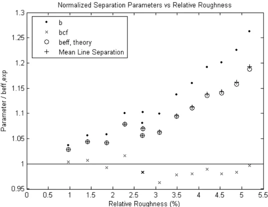
param-eters proposed by Taylor et al. [25] and Kandlikar et al. [26]. Based on the results, the Brackbill and Kandlikar works proposed a new constricted hydraulic diameter parameter.

(21)

to be used in calculating the friction factor. This new parameter is used in place of the

hydraulic diameter, and was found to give results that correspond to classic theory more

closely as seen in Figure 1.3 from Brackbill [29], where normalized results are shown as

a function of relative roughness. In this plot a value of1 represents agreement with

the-ory. It is easily seen that the constricted parameter better predicts fluid flow characteristics

[image:21.612.189.457.239.446.2]

compared to the root separation.

Figure 1.3: Constricted Parameter Performance

Wagner and Kandilkar [31] extended the work of Brackbill [28, 29] to incorporate

wall functions in the two dimension domain. Lubrication theory was used to extract a

pressure flow relationship to be used in the boundary layer analysis. The extension brings

inertial effects back into the flow physics to arrive at a velocity profile as shown in Equation

(1.10), wheref(x)andh(x)are continuous functions describing the bottom and top walls

respectively. The resulting expressions for friction factor were validated with experimental

(22)

u= 6 ˙V

z(h(x)−f(x))3 (y−f(x)) (y−h(x)) (1.10)

1.2.3

Heat Transfer

In 2001, Joshi [30] and Kandlikaret al.[34] studied the effects of surface roughness on flow characteristics. The work studied two stainless steel capillary tubes with diameters of 620

µmand 1067µmand relative roughness ranging from0.161%to0.355%, where Reynolds

number ranged from 500 to 3000. A reservoir and positive displacement pump were

uti-lized to pump distilled water through a flow meter controlling the mass flow rate in the

system. A needle valve was placed after the flow meter to help mitigate oscillations in the

flow throughout the system. The distilled water would then enter the test section. Pressure

drop was measured across the entire test section. For the heat transfer portion of the work,

DC electrical resistive heaters provided a constant heat flux across the capillary tubes. The

system was insulated with fiberglass insulation in order to minimize heat loss. Due to a low

current path being created were the pressure taps where machined, two sets of capillary

tubes were manufactured to run the pressure drop and heat transfer experiments separately.

In order to measure wall temperature, K-type thermocouples were attached to the exterior

walls of the capillary tubes at three places along the test pieces. Inlet and outlet

tempera-tures were measured in-line with jacketed K-type Thermocouples. Experimental data was

collected via LABVIEWTM_{. The work found that for smaller tubes, surface roughness was}

a significant factor in both heat transfer and pressure drop. The large tube of 1067 µm,

however, behaves as a macroscale tube.

Dharaiyaet al.[32] performed a numerical analysis of microchannels subject to the H2 boundary condition. The H2 boundary condition is defined as a constant heat flux along the

channel walls both axially and circumferentially. The numerical work varied aspect ratio

(23)

heating case was validated with published data to ensure the accuracy of the numerical

model. The investigation went further to return results for the fully developed Nusselt

number for two and three wall heating. These results for two wall heating are the only data

(24)

Chapter 2

Theoretical Analysis

The motivation exists to develop relationships that accurately predict physical situations.

These expressions allow engineers to properly design to meet specific application

require-ments. In most applications, however, full solutions to fundamental problems are not

possi-ble to obtain. For this reason it is often necessary to look toward analytical approximations

and theoretical limits to obtain bounds for design.

2.1

Complete Solution

Limiting theoretical cases with full, close-form solutions provide both insight and building

blocks for further refinement. In this section the classical case of parallel flat plates is first

investigated to provide the ultimate limit for Nusselt number. The results of Wagner [31]

for fluid flow in small aspect ratio channels with rough walls are then applied to the heat

transfer application.

2.1.1

Classical Parallel Flat Plates

The first approach to understanding the physics of heat transfer in small, wide channels

was to look at the limiting case of pressure driven flow between infinite parallel flat plates.

This case is a classical fluid mechanics problem found in textbooks. If we were to look

at the results from the Navier-Stokes equation for steady, fully developed, laminar,

(25)

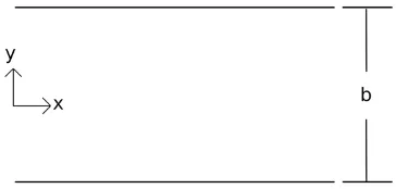
profile, where u is the axial velocity component with y = 0 centered between the plates

[image:25.612.226.408.168.255.2]

andbis the total gap size as shown in Figure 2.1

Figure 2.1: Smooth Channel Domain Illustration

~

V →u= 1 2µ

dP dx

y2− b 2

4

(2.1)

Next we look at the full energy equation in Equation (2.2).

ρCP

DT

Dt =ρqgen+∇ ·(k∇T) + DP

Dt +τ

0dui

dxi

(2.2)

Where DT_Dt and DP_Dt represent the total derivatives of temperature and pressure respectively.

The viscous dissapation terms are given in the last term on the right hand side,τ0dui

dxi

Apply-ing the additional standard assumptions of constant heat flux, no heat generation, constant

thermal conductivity and negligible viscous dissipation, energy reduces to:

u∂T ∂x =αf

∂2_T

∂y2 (2.3)

Since we are applying the constant heat flux boundary condition, we know that ∂T_∂x

(26)

later to ensure its accuracy. We are now left with an easily solvable, well-posed ordinary

differential equation:

uD=αf

d2_T

dy2 (2.4)

With the following boundary conditions on the first derivative:

∂T ∂y

y=−b

2

= −q

k

∂T ∂y

y=b

2

= q

k

This problem can be solved directly, but we are left with an integration constant. We

apply the fact that at the top or bottom plate, the fluid temperature is equal to the wall

temperature to pick up the last constant and close the solution.

T|b

2 =Tw(x) (2.5)

After applying this last boundary condition, we obtain an expression for the temperature

within the fluid across the gap:

T = q

k

₋

y4 b3 +

3y2 2b −

5b

16

+Tw (2.6)

When checked, the final expression forT satisfies the original ODE, validating setting

∂T

∂x equal to an arbitrary constant,D. The reason this works is becauseD, though arbitrary,

is a slave to the wall heat flux boundary conditions.

(27)

Tm =

1 ¯

vbz

Z ₂b

−₂b

uT zdy (2.7)

Substituting Equations (2.1) and (2.6), we can solve the integral exactly:

Tm =

17 70

q

kb+Tw (2.8)

The last step is to look at the definition of convection:

Q= ¯hA(Tw −Tm) (2.9)

This means the convective coefficient will equal:

¯

h=

Q A

Tw−Tm

(2.10)

Which, when the wall heat flux conditions and Equation (2.8) are applied, reduces to:

¯

h= 140k

17b (2.11)

Now we define Nusselt number based on the total separation,b:

N ub =

¯

hb

k =

140

17 ≈8.235 (2.12)

(28)

2.1.2

Wavy Walls

The objective is to be able to analyze structured roughness along the walls. In order to

incorporate non-smooth walls, we specify wall functions at the top and bottom walls as

h(x) and f(x) defining the wall topography. Each wall is only a function of the axial

direction and is continuous. The first approach is to adjust the velocity profile for a wavy

wall case and again perform the analysis from Section 2.1.1. The velocity profile that

will be used is based on a lubrication theory approximation. In order to use this velocity

profile, we are assuming a small slope trajectory between fluid particles as taken in Wager

and Kandlikar [31]. This theory was developed for dealing with small asperities found on

the walls in bearings. The small slope assumption dictates that the axial velocity profile is

approximately parabolic provided their are no sudden changes in a fluid particles trajectory.

Inertial effects have also been reincorporated into the velocity profile shown in Equation

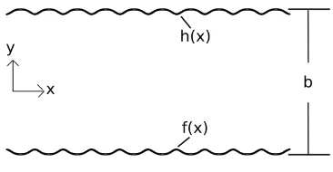
(2.13). A visual representation of the computational domain is illustrated in Figure 2.2.

The separation,b, is defined as the root separation or the distance between the average floor

[image:28.612.225.408.475.570.2]

profiles of each wall.

Figure 2.2: Wavy Wall Domain Illustration

u= 6 ˙V

(29)

Using the velocity profile from Wagner and Kandlikar [31] in the ordinary differential

equation given by Equation (2.4), and applying the same boundary conditions of constant

heat flux at the wall, we obtain a temperature profile within the fluid:

T = q

k(f(x)−h(x))3[y

4₋₂₍_f₍_x_{) +}_h₍_x₎₎_y3_{+ 6}_f₍_x₎_h₍_x₎_y2 _(2.14)

+ (f(x)3−3f(x)2h(x)−3f(x)h(x)2+h(x)3)y

−f(x)h(x)(f(x)2−3f(x)h(x) +h(x)2)] +Tw

In the case wheref(x)andh(x)are constant (smooth walls) the resulting temperature

profile reduces exactly to that of the smooth case. When the analysis is carried through to

the end, we obtain the following expression for Nusselt number based on the root

separa-tion:

N ub =

140b

17(h(x)−f(x)) (2.15)

Which again, reduces to conventional theory when h(x)−f(x) = b. Unfortunately,

upon further inspection, except in the case of smooth walls and possibly some

coinciden-tal wall functions, the expression obtained in Equation (2.14) fails to meet the criteria of

∂T

∂x being equal to a constant. We can conclude that the theoretical Nusselt number will

vary locally in wavy walled channels. However, if the difference of the wall functions is

replaced by the constricted parameter as is done by Brackbill [29], we obtain an acceptable

expression for Nusselt number.

N ub =

140b

17bcf

(30)

The constricted parameter is defined as:

bcf =b−2εf p (2.17)

2.2

Scale Analysis

In order to develop an understanding of the complex physics involved in the coupled

trans-port problem, the use of a scale analysis allows for the identification of dominant terms.

This approach provides insight without obtaining a full solution to sets of equation that

would otherwise have no closed form solution. If one were to apply lubrication theory as

done by Wagner [31] to the wavy wall setting, we could extract thexˆdirection of

momen-tum and continuity as shown in Equations (2.18) and (2.19).

ρ

u∂u ∂x +v

∂u ∂y

=−∂P ∂x +µ

∂2_u ∂x2 +

∂2_u ∂y2 +

∂2_u ∂z2

(2.18)

∂u ∂x +

∂v

∂y = 0 (2.19)

(31)

u=< v > u∗

x=Lx∗

y=by∗

z =az∗

P =PsP∗

wherePs is a scale chosen to balance appropriately with the right hand side. From

conti-nuity we can arrive at the scaledyˆvelocity,v:

v = b

L < v > v ∗

By applying our scaled quantities to Equation (2.18) we obtain the following:

ρ < v >2 L

u∗∂u ∗ ∂x∗ +v

∗∂u∗

∂y∗

=−Ps L

∂P∗

∂x∗ +µ < v >

1

L2 ∂2_u∗ ∂x∗2 +

1

b2 ∂2_u∗ ∂y∗2 +

1

b2 ∂2_u∗ ∂z∗2

(2.20)

By extracting the coefficients and rearranging, an expression is found that balances the

order of the terms:

Ø [αRe] = Ø

bPs

µ < v >

+ Ø

L a

+ Ø

"

b a

3#

+ Ø

"

b L

2#

(2.21)

(32)

side will be dominated by the pressure term and the L_a term. If we look at a length scale on

the order ofaand choose ourPs as shown below, then we are left with the dominant term

on the left hand side ofαRe. This parameter will be used as in reporting the experimental

results as it is a dominant term in the physics. This method is by no means a complete

solution, but lends insight into the complex problem.

Ps=

µ < v >

b (2.22)

The value of a scale analysis is in its to extract understanding of the fundamental physics

from the governing equations without applying additional simplifying assumptions. In this

case we were able to arrive at a term useful in comparing results from different geometries

on an equal basis. The utilization ofαRe, in a sense, normalizes results for channel aspect

ratio by dividing out this geometry factor. As will be seen later, the usefulness of this

(33)

Chapter 3

Experimentation

3.1

Experimental Setup

The experimental setup design used for this study is the next iteration of a previously proven

design for fluid flow characterization by Brackbill and Kandlikar [27,28]. The conceptual

auxiliary architecture and footprint of the design is maintained with the exception of

ma-terial selection and separation control. The design was of mutual acceptance for both of

the simultaneous heat transfer and fluid flow studies. Due to the requirement of precise

machining, the final manufacturing of complex auxiliary parts was performed via CNC

un-der the operation of NSF team member Brian LaPolt, Mechanical Engineering Technology,

Rochester Institute of Technology. The strength of the design is interchangeability of the

specially designed roughness test sections. Any arbitrary test section can be tested for both

fluid flow characteristics and heat transfer performance with directly compatible results.

Extensive consideration was placed on the design of the test sections. A previous

in-house, heat transfer experimental design showed unacceptable results due to the domination

of axial conduction within the test section. Learning from this case, the new test pieces

would have to account for this arising issue. An investigation was performed into the

(34)

had a number of factors to balance. The driving forces for the design were to minimize

axial conduction (multidimensional conduction within the wall), to ensure the footprint

of the test sections fit the predefined auxiliary architecture, allow for the application of a

heater, to support the placement of thermocouples, and to allow for a means of controlling

separation and maintaining a seal.

Axial conduction is a physical attribute that is governed by material and geometry.

Utilizing Equation 1.2, the non-dimension axial conduction number,M, can be calculated

for the desired range of Reynolds numbers, dimensions, and materials. The parameterM is

a measure of the ratio of conduction within the wall, along the length of the channel to the

convection from the wall to the fluid. Ana priorimeans can be performed to estimate Axial conduction using the experimental design. A simple ExcelTM _{whorksheet is utilized to}

estimate the parameterM.

The most desirable material for machining purposes is an Aluminum Alloy. Due to

the relatively high thermal conductivity of Aluminum (238_mW_·_K at 100◦C for Al6061-T6), low Reynolds number cases will have significant axial conduction. The plot in Figure

3.1 shows the worst case estimation forM as a percentage over Reynolds number for the

defined thickness of4mm(thickness required for rigidity and machinability for both

Alu-minum and Stainless Steel). Since axial conduction is considered negligible for values less

than1%, Aluminum Alloys are not acceptable for mitigating the effects of axial conduction.

The only reasonable option for material, despite complications in fabrication, is Stainless

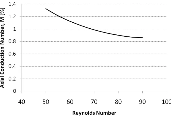
Steel. In order to establish a rule-of-thumb for a minimum Reynolds number, Figure 3.2 is

generated in the same fashion in order to show the low Reynolds number behavior of the

designed test section with the specified stainless steel. By inspection, a Reynolds number

of70can be used as a lower bounds for negligible axial conduction.

The available footprint, heater requirement, and base design for fluid flow directed the

(35)

[image:35.612.180.460.127.321.2]

Figure 3.1: Axial Conduction,M Comparison of Aluminum and Stainless Steel

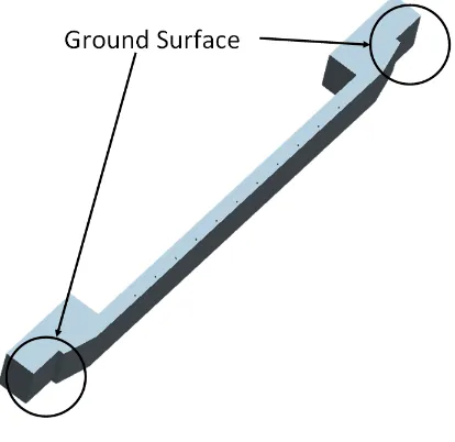
[image:35.612.175.473.439.643.2]

(36)

of specific surfaces: ground ends, angled headers, channels walls, and heater attachment

locations. Thermocouple holes are drilled to the center of each test piece in eleven locations

equally spaced by6.35mm.

The ends of each test piece have to have a ground face in order to support the gauge

blocks. This surface is identified in Figure 3.3 on either end. These surfaces are ground

smooth to meet two functions, first, the geometric tolerance of the system require careful

[image:36.612.219.426.273.474.2]

care, and second, these surfaces mate with the gauge blocks to create a water tight seal.

Figure 3.3: Test Piece Ground Surfaces

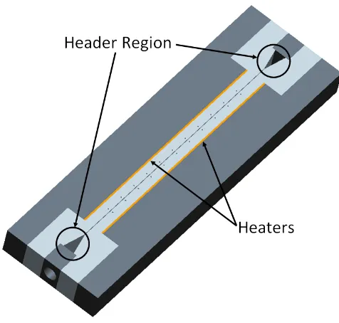
The next surface is an angled surface to act as the header for the channel. These surfaces

direct the flow from the gauge block down to the final channel root separation. When the

two test pieces are assembled in the test section, they make a triangular header region at

both the inlet and outlet as shown in Figure 3.4. The design, in conjunction with the gauge

blocks, is meant to ensure a smooth transition from circular to rectangular ducts. The

channel exit is symmetric with the inlet, and so has the same header configuration.

(37)

[image:37.612.208.446.88.315.2]

Figure 3.4: Test Section Assmebly

elements making up the channel walls. The design creates a total length of 114.6 mm

for hydrodynamic flow with a channel height of 12.7 mm. These surfaces are machined

using a wire Electrical Discharge Machining technique to provide the specified controlled

geometries.

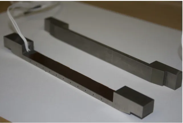
Lastly, the test pieces must provide a footprint for the application of heaters. Silicone

Film heaters with adhesive backs rated at10W were identified. The total heated area has

a length of94.6mmand height spanning that of the channel wall, 12.7mm. Figure 3.5

shows an example picture of the smooth test pieces.

The gauge blocks, as illustrated in Figure 3.6, act as the means of controlling separation,

provide the transition point from the circular inlet tube to the square channel geometry,

and provide the mating surface to seal the channel ends with the test pieces. The overall

geometry for different gauge blocks is maintained with the exception of varying width

for varying separations. The detailed drawings of the gauge blocks can be found in the

(38)

[image:38.612.164.485.123.338.2]

Figure 3.5: Test Piece Example

[image:38.612.259.383.452.628.2]

(39)

The heat transfer aspect of the study magnifies the requirements of the experimental

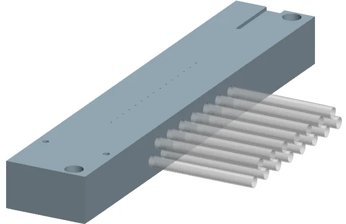
setup. First, the heat transfer setup requires an insulating enclosure, and so, the ceramic

Garolite G-10, a resin based ceramic, was selected due to its low thermal conductivity of

0.288_mW_·_K, operating temperature range, and acceptable machinability. The base block, as illustrated in Figure 3.7, provides a smooth mounting surface with fifteen pressure taps

spaced equally by 6.35 mm along the total length of the flow channel. Low durometer

(highly compressible) silicone gasketing with an ample operating temperature range was

selected to accommodate the extra sealing requirement around the thermocouple wires.

Gaskets were cut to fit the base block and cover pieces. These low durometer gaskets were

chosen to ensure sealing around the channel edges and thermocouples. Setup clamps are

[image:39.612.153.493.357.577.2]

used to compress the test section and gaskets.

(40)

3.2

System Architecture

Brackbill and Kandlikar implemented a variable hydraulic diameter test setup [27,28].

For the proposed work, the test setup remains nearly the same from a system architecture

stand point. The only difference in architecture is the addition of a constant temperature

water bath and heat exchanger subsystem to meet the heat transfer conditioning needs.

Figure 3.8 below shows a representation of the overall system. Degassed, distilled water

is circulated through the system by a Micropump motor drive attached to a Micropump

positive displacement, micro-geared metered pump head. The system is capable of up to

2500 mL/min with 8 bars of pressure drop. The working fluid exits the closed reservoir

and is conditioned through a heat exchanger with an outside loop cooled by a chiller at

a constant temperature. The reservoir is necessary to ensure the water remains degassed.

The heat exchanger is used in order to avoid cavitation issues that arise from the chiller

being physically below the test section. The working fluid exits the heat exchanger and

flows through a bank of flow meters to monitor the flow rate. The flow meter bank includes

a bypass loop and two digital flow meters. The two flow meters in parallel are capable of

measuring 10-100 mL/min and 60-1000 mL/min respectively. The use of a flow meter bank

in this fashion will increase the accuracy per given range of flow. The degassed, distilled

water exits the flow meter on its way to the test section. After exiting the test section, the

working fluid is returned to the reservoir.

3.3

Measurements

The measurable quantities for this experimental setup are volumetric flow rate, pressure

drop between two pressure taps, fluid inlet and outlet temperature, and wall temperature.

(41)

Figure 3.8: System Architecture

The pressure can be measured at known locations along the length of the channel. The

inlet fluid temperature is measured by a jacketed K-type thermocouple. Upon exiting the

test section, the total temperature is again measured by the same means. Channel wall

temperature is more difficult to obtain. Thermocouples are made out of 36AWG K-type

thermocouple wire via an in-house thermocouple welder using nitrogen as the inert gas.

The thermocouples are inspected under a microscope to ensure proper welding as can be

seen in Figure 3.9. The thermocouples are then dipped in thermal-epoxy to protect exposed

wire from water contact.

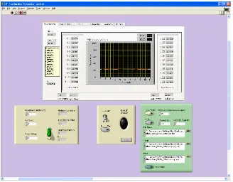
A robust, well-organized LABVIEW GUI as shown in Figure 3.10 was developed in

order to facilitate the collection of measurable quantities. The LABVIEWTM_{code was}

opti-mized for ease of use during heat transfer testing. Sensor information is visually presented

to facilitate ease of reading and accurately performing tests. The code records calibrated

raw data obtained from sensors. Parameters recorded are listed below.

(42)

2. Fluid Temperatures:Tin,Tout

3. Pressure Drop: ∆T

4. Wall Temperature: Ti,i= 1,2,3, ...,11

Where the thermocouples are located in the center of the4mmwall thickness, at the center

of the depth, and at the axial distances of (measured from the start of the heated channel):

1. 16.2mm

2. 24.4mm

3. 32.7mm

4. 40.9mm

5. 49.1mm

6. 57.3mm

7. 65.6mm

8. 73.8mm

9. 82.0mm

10. 90.2mm

11. 98.5mm

3.4

Roughness Geometry Design

The effect of the ratio of pitch to height of structured roughness elements has been

iden-tified as a key parameter on fluid flow and heat transfer [31]. In this study the sinusoidal

(43)

[image:43.612.161.489.377.633.2]

Figure 3.9: 36AWG Thermocouple Weld

(44)

The general form of the designed curve is shown in Equation (3.1). The actual fabricated

surfaces varied slightly as is discussed in the Results section. The surfaces are tested in

both concurrent fluid flow and heat transfer studies. The explicit designed parameters are

listed in Figure 3.11.

y(x) = hhcosπ λx

iP

(3.1)

Figure 3.11: Structured Roughness Design Parameters

3.5

Assembly

3.5.1

General Assembly

The assembly of the test setup proves to be the most important step in the experimental

procedure. Prior to any testing, the adhesive backed heaters are attached to individual test

sections and allowed to cure for 72 hours per manufacturer specifications. The auxiliary

setup is fitted with appropriate gaskets and mounted on the experimental stand. The

sys-tem is ran as a closed loop without the test section to ensure proper performance. Once

prepared, the test sections are carefully cleaned with small amounts of Isopropyl Alcohol

(45)

materials as shown in Figure 3.12. The test section is mounted on the base block and

se-cured axially and laterally. With the test section securely placed, the 22 thermocouples are

covered in thermal paste and carefully placed in their respective locations. The

thermocou-ple holes are designed to place the weld at the center of the channel wall. At this point,

the channel separation is measured via a optical confocal microscope. Figure 3.13 shows

the assembled setup being measured by the microscope. Once the separation is accurately

measured and checked along the length of the channel, the test setup is sealed with the top

plate. Serrated step clamps are used to apply a constant force for vertical sealing.

Figure 3.12: Test Setup Assembly

3.5.2

Power Balancing

Due to manufacturing variations individual heaters will vary slightly in resistance. In order

to balance the power being applied to each wall a potentiometer was placed in series with

each resistive heater. This creates two series circuits with one heater and one potentiometer

each. These circuits are then placed in parallel with nodes at the positive and negative

terminals of the system power supply. The resistance of each heater is measured along with

(46)

Figure 3.13: Test Setup Assembly

“zero” setting. A simple circuit analysis is performed using Ohm’s law. An Excel sheet

was created in order to utilize solver to minimize the difference in power output by each

heater. This method allows for the heaters to be balanced within0.1%at room temperature.

3.6

Conditioning

3.6.1

Sensor Calibration

Accurate measurement is an essential aspect of any experimental study. For this reason

care is taken in order to ensure information gathered from sensors is properly interpreted.

The experimental setup in this study has three types of sensors that need to be calibrated.

There are a set of differential pressure sensors, the flow meter bank, two jacketed K-Type

thermocouples and 23 K-Type thermocouples made from the 36AWG wire.

The first sensor is the set of Huba Control differential pressure sensors type 692 used

in calculating pressure drop. A0.1bar and0.2bar pressure sensor with reported0.4%F S

(47)

known pressures by means of the in-house digital pressure calibrator. Pressure and voltage

are recorded within the linear range of the piezoelectric device. Least squares is then used

on the recorded calibration points to quantify the linear relationship between pressure and

measured voltage. An example calibration curve is shown in Figure 3.14 This procedure

is repeated for each sensor and is checked to ensure the sensors have not deviated during

[image:47.612.181.450.239.448.2]

testing.

Figure 3.14: Pressure Sensor Calibration Curve

The second set of sensors is the two Omega digital flow meters type FLR1000. The two

ranges of 10-100 ml/minand 100-1000 ml/minwith reported accuracy of1%F S were

selected. In an analogous way, water is pushed at a constant rate through the individual

flow meter. Both time and mass of fluid are recorded for at least 60 seconds. For lower

flow rates a digital scale is used to accurately measure the mass of the fluid, while higher

flow rates require a triple beam balance due to the limit of the digital scale. Mass and time

measurements are converted to volumetric flow rates and then the least squares method

is again employed to find the quantitative relationship between sensor output voltage and

(48)

[image:48.612.191.452.121.329.2]

ml/min).

Figure 3.15: Flow Meter Calibration Curve

The last set of sensors is the large array of thermocouples. These sensors are calibrated

using a two-point approach to find the slope and intercept of the calibration curve. A

bath of distilled water at the local two-phase points (freezing and boiling) is first prepared.

The sensors, once protected with epoxy or their inherent jacketing are submerged in the

prepared baths while voltage is measured. This method proves to be extremely accurate in

obtaining calibration data.

3.6.2

Heat Loss Tests

Garolite has a very low thermal conductivity of 0.288 _W

m·K

, however, it is not a perfect

insulator. In order to account for all system losses, it was necessary to perform heat loss

tests. The setup was first assembled in the same fashion as described in Section 3.5 with

plain smooth channels. No water was introduced to the setup during the tests. A known

(49)

along with average wall temperature and ambient temperature. The entire setup was

al-lowed to reach steady state, which took approximately 30 minutes for each power setting.

Steady state was ensured by recording temperature readings for 15 minutes and checking

the standard deviation of the readings was less than experimental error in temperature.

It is assumed that the total power reading is the same as the heat loss when fluid flow is

not present. By varying input power and recording steady state temperatures, a plot of heat

loss as a function of the temperature difference of the average wall temperature, Tave and

ambient temperature can be generated. It was predicted and shown to be true that heat loss

has a linear relationship with the temperature difference (∆T =Tave−TRoom). Figure 3.16

shows the resulting curve and a linear regression for these tests. This slope of this curve is

used in Equation (3.3) for heat loss estimations.

Tave =

Tave,wall1+Tave,wall2

2 =

1 11

11

X

i=1

Ti,wall1+

1 11

11

X

i=1

Ti,wall2 (3.2)

qloss= 0.16265(Tave−Troom) (3.3)

3.6.3

Fluid Flow Only Validation

Before any heat transfer tests were performed, the entire test system was validated for fluid

flow only conditions. These tests were performed on the smooth channels with varying

separations (aspect ratio) and Reynolds number. Pressure, fluid temperature and flow rate

were collected in order to calculate friction factor, f, based on Equation (3.4). Results

were compared to convention theory as defined by Equation (3.5) from Kakac et al.[33].

(50)

[image:50.612.169.463.96.303.2]

Figure 3.16: Heat Loss Curve

typical of the setup’s compliance with conventional fluid flow smooth theory. Validation

was ensured for the four separations of165µm,338µm,501µm,593µmwith the smooth

test section.

f = ∆P

x

ρDhA2

2 ˙m (3.4)

f = 24

Re 1−1.3553α+ 1.9467α

2₋₁_.₇₀₁₂_α3_{+ 0}_.₉₅₆₄_α4₋₀_.₂₅₃₇_α5

(51)

[image:51.612.182.468.91.304.2]

Figure 3.17: Experimental Friction Factor Compared to Conventional Theory

3.7

Operation

In order to ensure consistent results, a test procedure was developed and maintained for

the duration of testing. Once the assembly procedure listed in Section 3.5 has been carried

out, LABVIEW is opened and the test parameters entered. The LABVIEW GUI only

requires separation information to begin a test. The heaters are powered by an external

power supply, flow rate is controlled via the GUI, and minor manual dexterity is required

to choose the appropriate flow meter and pressure sensor.

Once the micropump is started, the first step to starting a test is to ensure there are no

leaks around the test setup. If the setup does not leak, the power supply is turned on and

set to the proper voltage of a given test. The constant temperature bath is also set to control

the inlet temperature to the test section. The setup is allowed to come to steady state by

waiting for approximately 30 minutes. Once steady state is ensured, data is recorded over

a 12 minute interval. The data is checked to ensure temperature variation in the form of the

(52)

set point. If the power has not been changed, it takes approximately 15 minutes for steady

state to be reached. Data is again recorded and the procedure is repeated over the entire test

range.

It is important to constantly look for leaks. Garolite, being a resin based ceramic, does

not leave surfaces that are as smooth as aluminum, and so does not seal as well, especially

at non-gasketed interfaces. If leaking is observed, the test is stopped, data discarded, and

reassembly is performed. The regions most prone to leaking are in the header regions. The

proper cutting of gaskets is essential in creating a water tight setup. Slight mis-alignment

of test section and gasket will cause a leak. Fortunately, the heaters used in the setup are

designed with PTFE coated wires, and will resist the incidental water contact. The heaters,

(53)

Chapter 4

Data Processing

4.1

Surface Analysis

Geometry of roughness surfaces can be hard to establish when working on the order of

mi-crons. For this reason a Keyance Confocal Laser Scanning Microscope (model# VK9710)

was utilized for surface analysis. Each roughness surface was imaged using the Keyance

VK Analyzer software, providing the require topography information to analyze each

[image:53.612.156.463.470.678.2]

sur-face geometry.

(54)

Figure 4.2: Curve Fit Coefficients

Topography data was extracted for processing in Excel. The average roughness of

the smooth channel pieces was extracted directly and found to be 1 µm. The structured

roughness surfaces require some sophistication in order to properly quantify their surfaces.

A curve fit was performed using Solver to minimize the residuals between the surface

topography and the desired form of the surface model shown in Equation (4.1). The form

of the equation can be generalized to fit the form of the output data. The general form to

which each surface was fitted is shown in Equation (4.2)

f(x) =hhcosπ λx

iP

(4.1)

f(x) =a1[cos(a2x+a3)]a4 +a5 (4.2)

Using the topographical information extracted, curve fits where performed to each of

the four surfaces shown in Figures 4.3 through 4.6. The resulting coefficients for each

(55)

Figure 4.3: Surface Rendering ofλ/h= 2.6

(56)

Figure 4.5: Surface Rendering ofλ/h= 7.8

(57)

4.2

Data Reduction

Care was taken to properly process collected data. For heat transfer tests there were a

number of steps that had to be taken prior to reaching the final result of average fully

developed Nusselt number. The process flow for each of the data sets is the same and can

be summarized in seven steps:

1. Raw data is recorded by LABVIEW in the form of thermocouple readings, flow rates,

geometry, and experimental conditions.

2. Raw data is compiled in a single Excel worksheet for each separation and geometry.

3. A custom VBA script extracts relevant data while performing an initial statistical

analysis where appropriate.

4. Parameters from all data sets are combined in single worksheet for further data

pro-cessing.

5. The first stage of processing calculates derived geometric parameters, fluid

proper-ties, length of the developing region, and total heat flux.

6. The results from the first stage of processing are used in the second stage of

process-ing, which is performed in a summary worksheet combining all geometries.

7. The second stage of processing calculates local nusselt number as shown in Equation

(4.17) for each thermocouple as well as the uncertainty of each result.

In the first step, data collection, the procedure for testing outlined in Section 3.7 was

followed to ensure proper, consistent testing. The LABVIEWTM_{GUI is used to actively}

control the experiment. The user inputs geometric and test information before beginning

(58)

outlet fluid temperature, room temperature, and wall temperatures are acquired from the

setup’s thermocouples. Flow rate and geometry information are also recorded by the code.

Each test condition creates a single, archival raw data sheet. In order to organize the

raw data in a usable fashion, the second step is performed combining results from a single

separation and geometry in a single worksheet. The custom VBA script is run, organizing

the data, averaging flow rate and fluid temperatures, and preparing the wall temperatures.

The fourth step takes the results in their new form and combines them for each

indi-vidual geometry. This allows the data to be organized in a format that allows comparison

within a single geometry. The first steps of data processing are performed in this sheet.

First, the geometric information about separation and surface geometry is used to derive

secondary geometric parameters. Hydraulic diameter is then calculated using Equation

(4.3) and aspect ratio is defined as Equation (4.4). The last standard geometric parameter,

relative roughness can be calculated using Equation (4.5). Figure 4.7 shows a cross section

[image:58.612.239.405.432.535.2]

view of the channel with axial flow into the page.

(59)

Dh =

4ab

2(a+b) (4.3)

α= b

a (4.4)

ε/D= εf p

Dh

(4.5)

∆T =Tout−Tin (4.6)

Next, the constricted parameter can be calculated by Equation (4.7). This parameter can

then be used to calculate the constricted hydraulic diameter and aspect ratio by replacingb

withbcf.

bcf =b−2εf p (4.7)

Fluid temperatures are then used to find the mean fluid temperature to be used in the

interpolation of the Prandtl number, viscosity, and thermal conductivity. The total

temper-ature change across the fluid is used to calculate the power input with Equation (4.8).

Q= ˙mCp∆T (4.8)

Reynolds number is now calculated followed by the developing length for a given

(60)

be used to identify which wall thermocouples are in the fully developed region.

Re= 4 ˙m

2µ(a+b) (4.9)

xf d = 0.05ReP rDh (4.10)

The last parameters that need to be defined in this stage of the data processing are the

two different heat flux calculations. Heat flux is calculated using the projected area (size of

the heater), and using an estimate of the actual area including roughness. The actual area

is estimated by the arclength of one roughness element over the pitch as found in the curve

fitting in Section 4.1.

qP =

Q AP

(4.11)

qactual =

Q

Aactual

(4.12)

At this point the partially processed data can be combined in a summary data sheet

along with the average wall temperature at each of the 11 locations. Internal wall

tem-perature, which is in contact with the fluid, can be estimated by a simple wall conduction

analysis as seen in Equation (4.14), where all temperatures are in Kelvin[K].

∆T = q

ks∆x

(4.13)

Tw =Ti−∆T =Ti−

q

(61)

The fluid temperature at any location can be estimated assuming a linear axial increase

along the heated length (due to the constant heat flux boundary condition).

Tf =

Tout−Tin

LH

x+Tin (4.15)

The last two temperature can then be used to find the difference in mean fluid

tempera-ture and the internal wall temperatempera-ture at any thermocouple location. The local heat transfer

coefficient can now be defined by Equation (4.16) and calculated for all fully developed

locations from a given test set.

¯

h= q

Tw−Tf

(4.16)

It is important to note that both the wall temperature, Tw, and the local heat transfer

coefficient can be calculated using the actual and projected areas. The actual area will

Exploration of the effect of surface roughness on heat transfer in microscale liquid flow