A comprehensive study of footing on c-φ soil slopes - numerical and physical modelling

University of Southern Queensland

Faculty of Engineering and Surveying

A Conprehensive Study of Footing on

c--

φ

Soil Slopes -- Numerical and

Physical Modelling

A dissertation submitted by

Andrew James Shorten Cole

In fulfilment of the requirements of

Courses ENG4111 and ENG4112 Research Project

towards the degree of

Abstract

The problem of a footing being located on a slope is one which is encountered regularly and must be understood so that catastrophic failure of structures causing death or injury does not occur. This research project is split into two different but still related sections aimed at providing a greater understanding of the footing on slope problem.

This project will initially undertake a numerical study to see what effect geometrical and material properties have on the bearing capacity of a footing located on a slope, with non--dimensional parameters used to highlight these effects. These parameters include dimensionless strength ratio, footing distance ratio, slope height ratio and soil internal friction angle which in this paper have been analysed more comprehensively then previously done before. FLAC will be used as the analysing software with the results obtained from these analyses are presented in design charts making the information easy to understand and use.

University of Southern Queensland

Faculty of Engineering and Surveying

ENG4111 Research Project Part 1 &

ENG4112 Research Project Part 2

Limitations of Use

The Council of the University of Southern Queensland, its Faculty of Engineering and Surveying, and the staff of the University of Southern Queensland, do not accept any responsibility for the truth, accuracy or completeness of material contained within or associated with this dissertation.

Persons using all or any part of this material do so at their own risk, and not at the risk of the Council of the University of Southern Queensland, its Faculty of Engineering and Surveying or the staff of the University of Southern Queensland.

This dissertation reports an educational exercise and has no purpose or validity beyond this exercise. The sole purpose of the course ”Project and Dissertation” is to contribute to the overall education within the student’s chosen degree programme. This document, the associated hardware, software, drawings, and other material set out in the associated appendices should not be used for any other purpose: if they are so used, it is entirely at the risk of the user.

Prof Frank Bullen

Certification

I certify that the ideas, designs and experimental work, results, analyses and conclusions set out in this dessertation are entirely my own effort, exept where otherwise indicated and acknowledged.

I further certify that the work is original and has not been previously submitted for assessment in any other course of institution, except where specifically stated.

Andrew James Shorten Cole

Student Number: 0050057529

_______________________________________ Signature

Acknowledgements

I would like to thank Dr. Jim Shiau for his support and professional advice whilst I undertook this project. His expert knowledge in the geomechanics field was always available for any problems encountered and his guidance was greatly appreciated throughout the year.

I would also like the thank Dean Beliveau for his time and effort put into the software used with the physical modelling. His input ensured a reliable program was created which proved very easy to use, and if any problems in the software were found he was more then happy to help rectify the situation.

Table of Contents

Abstract . . . ii

Limitations of Use . . . iii

Certification . . . iv

Acknowledgements . . . v

Table of Contents . . . vi

List of Figures . . . x

List of Tables . . . xiv

Nomenclature. . . xv

Project Introduction . . . . 1--1

1.1 Footing on Slope Problem Statement. . . 1--1

1.2 Research Aims and Objectives . . . 1--1

1.3 Clay and Sand Numerical Model Differences . . . 1--2

1.4 Brief Introduction to FLAC . . . 1--3

Literature Reviews . . . . 2--1

2.1 Introduction . . . 2--1

2.2 Shallow Foundations . . . 2--1

2.3 Bearing Capacities . . . 2--2

2.3.1 Ultimate Bearing Capacity . . . 2--2

2.3.2 Allowable Bearing Capacity . . . 2--2

2.4 Failure Modes . . . 2--3

2.4.1 General Shear Failure . . . 2--3

2.4.2 Local Shear Failure . . . 2--3

2.4.3 Punching Shear Failure. . . 2--4

2.5 Footing on Flat Ground Theories . . . 2--5

2.5.1 Terzaghi’s Level Ground Bearing Capacity Theory . . . 2--5

2.5.2 Meyerhof’s Level Ground Bearing Capacity Theory . . . 2--6

2.5.3 Additional Researchers . . . 2--7

2.6 Footing on Slope Theories . . . 2--8

2.6.1 Meyerhof’s Footing Near Slope Bearing Capacity Theory . . . 2--8

1

2.6.4 Additional Researchers . . . 2--9

2.7 Previous Research Work Done . . . 2--9

2.7.1 Biopuso Samuel (2005). . . 2--9 2.7.2 Catherine Smith (2006) . . . 2--9 2.7.3 Joshua Watson (2008) . . . 2--10 2.7.4 Matthew Arnold (2008) . . . 2--10 2.7.5 Nathan Lyle (2009). . . 2--11

Validation of FLAC Software for c−φ Soil Analysis . . . . . 3--1

3.1 Introduction . . . 3--1 3.2 Effect of Applied Velocity. . . 3--2 3.3 Effect of Stepping Number . . . 3--4 3.4 Effect of Element Size . . . 3--6 3.5 Comparison with Other Existing Solutions . . . 3--9

Numerical Analysis -- 90˚Slope . . . . 4--1

4.1 Introduction . . . 4--1 4.2 Effect of Dimensionless Strength Ratio, c∕γB. . . 4--2

4.2.1 Comparison With Footing Distance Ratio . . . 4--4 4.2.2 Comparison With Slope Height Ratio . . . 4--6 4.2.3 Comparison With Friction Angle . . . 4--8 4.2.4 Conclusion. . . 4--10

4.3 Effect of Internal Friction Angle, φ . . . 4--10

4.3.1 Comparison With Dimensionless Strength Ratio . . . 4--11 4.3.2 Comparison With Footing Distance Ratio . . . 4--13 4.3.3 Comparison With Slope Height Ratio . . . 4--15 4.3.4 Conclusion. . . 4--17

4.4 Effect of Footing Distance Ratio, D_∕B . . . 4--17

4.4.1 Comparison With Dimensionless Strength Ratio . . . 4--18 4.4.2 Comparison With Slope Height Ratio . . . 4--20 4.4.3 Comparison With Friction Angle . . . 4--22 4.4.4 Conclusion. . . 4--24

4.5 Effect of Slope Height Ratio, H_∕B . . . 4--24

4.5.1 Comparison With Dimensionless Strength Ratio . . . 4--25 4.5.2 Comparison With Footing Distance Ratio . . . 4--27 4.5.3 Comparison With Friction Angle . . . 4--29 4.5.4 Conclusion. . . 4--31

4.6 Effect of Stability Number, N=c∕γHF . . . 4--31

4.6.1 Comparison With Footing Distance Ratio . . . 4--32

3

4.7.1 Footing on Flat Ground or Slope Condition Charts . . . 4--37 4.7.2 Increased Bearing Capacity With Increasing Strength Ratio

Charts . . . 4--38 4.7.2 Increased Bearing Capacity With Increasing Footing Distance Ratio Charts . . . 4--39 4.7.2 Decreased Bearing Capacity With Increasing Slope Height Ratio Charts . . . 4--40 4.7.2 Increased Bearing Capacity With Increasing Stability Number Charts . . . 4--41

4.8 Example of Chart Use . . . 4--41

4.8.1 Example 1 . . . 4--42 4.8.2 Example 2 . . . 4--44

Physical Modelling . . . . 5--1

5.1 Introduction . . . 5--1 5.2 Modelling Objectives . . . 5--1 5.3 Methodology . . . 5--2 5.4 Testing Procedures . . . 5--11 5.5 Results . . . 5--15

5.5.1 D/B = 0 . . . 5--16 5.5.2 D/B = 0.5 . . . 5--17 5.5.3 D/B = 1 . . . 5--18 5.5.4 D/B = 2 . . . 5--19 5.5.5 D/B = 3 . . . 5--20 5.5.6 D/B = 4 . . . 5--21 5.5.7 Comparison with Numerical Results . . . 5--22

5.6 Improvements for Future Physical Modelling . . . 5--24 5.7 Conclusion . . . 5--25

Conclusion. . . . 6--1

6.1 Results Summary . . . 6--1 6.2 Problems Encountered . . . 6--2

6.2.1 Numerical Modelling . . . 6--2 6.2.2 Physical Modelling . . . 6--3

6.3 Procedure Improvements . . . 6--4

6.3.1 Numerical Modelling . . . 6--4 6.3.2 Physical Modelling . . . 6--4

6.4 Future Work. . . 6--5

6.4.1 Numerical Modelling . . . 6--5 6.4.2 Physical Modelling . . . 6--5

5

References . . . . 7--1

Appendix . . . . 8--1

8.1 Appendix A -- Project Specification . . . 8--1 8.2 Appendix B -- Footing on Flat Ground or Slope Condition Charts

8--3 . . . . 8.3 Appendix C -- Increased Bearing Capacity due to Increasing

Strength Ratio Charts . . . 8--6 8.4 Appendix D -- Increased Bearing Capacity due to Increasing

Footing Distance Ratio Charts . . . 8--29 8.5 Appendix E -- Decreased Bearing Capacity due to Increasing

Slope Height Ratio Charts . . . 8--52 8.6 Appendix F -- Increased Bearing Capacity due to Increasing

Stability Number Charts . . . 8--61 8.7 Appendix G -- Data Used in Design Charts . . . 8--82

7

List of Figures

Figure 1.1:Typical jpeg output from FLAC . . . 1--4

Figure 1.2: Screenshot of FLAC software program . . . 1--5

Figure 2.1:General shear failure plane and load--displacement curve . . . 2--3

Figure 2.2: Local shear failure plane and load--displacement curve . . . 2--4

Figure 2.3: Punching shear failure plane and load--displacement curve . . . 2--4

Figure 2.4: Shear zones based on Terzaghi’s theory . . . 2--6

Figure 3.1:Validation for increasing y--velocity . . . 3--3

Figure 3.2: Validation for increasing stepping number . . . 3--5

Figure 3.3: 0.1 mesh size . . . 3--7

Figure 3.4: 0.5 mesh size . . . 3--7

Figure 3.5: Validation for increasing element size . . . 3--8

Figure 3.6: Comparison against other results . . . 3--10

Figure 4.1:Increasing bearing capacity with increased strength ratio . . . 4--3

Figure 4.2: Effect of dimensionless strength ratio with footing distance ratio . . . 4--4

Figure 4.3: Contour plots for dimensionless strength ratio with varied footing distance

ratio . . . 4--5

Figure 4.4: Effect of dimensionless strength ratio with slope height ratio . . . 4--6

Figure 4.5: Contour plots for dimensionless strength ratio with varied slope height ratio

4--7 . . . .

Figure 4.6: Effect of dimensionless strength ratio with friction angle . . . 4--8

Figure 4.7: Contour plots for dimensionless strength ratio with varied internal friction

4--9 . . . .

Figure 4.8: Effect of friction angle with dimensionless strength ratio . . . 4--11

Figure 4.10: Effect of friction angle with footing distance ratio . . . 4--13

Figure 4.11: Contour plots for friction angle with varied footing distance ratio . . 4--14

Figure 4.12: Effect of friction angle with slope height ratio . . . 4--15

Figure 4.13: Contour plots for friction angle with varied slope height ratio . . . 4--16

Figure 4.14: Effect of footing distance ratio with dimensionless strength ratio . . . 4--18

Figure 4.15: Contour plots for footing distance ratio with varied dimensionless strength

ratio . . . 4--19

Figure 4.16: Effect of footing distance ratio with slope height ratio . . . 4--20

Figure 4.17: Contour plots for footing distance ratio with varied slope height ratio 4--21

Figure 4.18: Effect of footing distance ratio with friction angle . . . 4--22

Figure 4.19: Contour plots for footing distance ratio with varied friction angle . . 4--23

Figure 4.20: Effect of slope height ratio with dimensionless strength ratio . . . 4--25

Figure 4.21: Contour plots for slope height ratio with varied dimensionless strength

ratio . . . 4--26

Figure 4.22: Effect of slope height ratio with footing distance ratio . . . 4--27

Figure 4.23: Contour plots for slope height ratio with varied footing distance ratio 4--28

Figure 4.24: Effect of slope height ratio with friction angle . . . 4--29

Figure 4.25: Contour plots for slope height ratio with varied friction angle . . . 4--30

Figure 4.26: Effect of stability number with footing distance ratio . . . 4--32

Figure 4.27: Contour plots for stability number with varied footing distance ratio 4--33

Figure 4.28: Effect of stability number with friction angle. . . 4--34

Figure 4.29: Contour plots for stability number with varied friction angle . . . 4--35

Figure 4.30: Footing on Flat Ground or Slope Condition Chart . . . 4--37

Figure 4.31: Increased Bearing Capacity with Increasing Strength Ratio Charts . . 4--38

Figure 4.32: Increased Bearing Capacity with Increasing Footing Distance Ratio Charts

4--39 . . . .

Figure 4.35: Example 1 slope scenario . . . 4--42

Figure 4.36: Design chart chosen for Example 1 . . . 4--43

Figure 4.37: Example 2 slope scenario . . . 4--44

Figure 4.38: Design chart chosen for Example 2 . . . 4--45

Figure 5.1:Overall view of Test Load Frame . . . 5--3

Figure 5.2: Linear actuator, transducer, load cell and steel plate configuration . . . . 5--4

Figure 5.3: Test tank construction . . . 5--6

Figure 5.4: Drill and attachment and bin used to mix material . . . 5--7

Figure 5.5: Initial load applied to the clay. . . 5--8

Figure 5.6: Load applied after 1 week . . . 5--9

Figure 5.7: Load applied 2 weeks after mixing . . . 5--9

Figure 5.8: Consolidated material cut ready for testing . . . 5--10

Figure 5.9: Clockwise from top left: obtaining triaxial test sample; trimming sample to

required length; final sample ready for testing . . . 5--12

Figure 5.10: Sample being subjected to triaxial test . . . 5--13

Figure 5.11: Sample ready for testing to begin . . . 5--14

Figure 5.12: D/B = 0 test sample . . . 5--16

Figure 5.13: D/B = 0.5 test sample . . . 5--17

Figure 5.14: D/B = 1 test sample . . . 5--18

Figure 5.15: D/B = 2 test sample . . . 5--19

Figure 5.16: D/B = 3 test sample . . . 5--20

Figure 5.17: D/B = 4 test sample . . . 5--21

Figure 5.18: Design chart used for numerical comparison . . . 5--22

Figure 5.19: Zoomed in design chart . . . 5--23

Figure B1--B4:Footing on Flat Ground or Slope Condition Charts . . . 5--23

Figure C1--C44:Increased Bearing Capacity due to Increasing Strength Ratio Charts .

5--23 . . . .

Figure E1--E16:Decreased Bearing Capacity due to Increasing Slope Height Ratio

Charts . . . 5--23

Figure F1--F40:Increased Bearing Capacity due to Increasing Stability Number Charts

List of Tables

Table 2.1:Example Terzaghi factor values . . . 2--5

Table 2.2: Example Meyerhof factor values compared with Terzaghi values. . . 2--7

Table 3.1:Applied velocity, stepping number, bearing capacity, CPU time . . . 3--3

Table 3.2: Stepping number, penetration depth, bearing capacity, CPU time . . . 3--5

Table 3.3: Applied velocity, stepping number, bearing capacity, CPU time . . . 3--9

Table 3.4: Results from comparison of methods . . . 3--11

Table 5.1:Comparison of physical and numerical results . . . 5--23

Table G.1:Data for H/B = 0 . . . 8--82

Table G.2: Data for H/B = 1 . . . 8--83

Table G.3: Data for H/B = 2 . . . 8--84

Table G.4: Data for H/B = 3 . . . 8--85

Table G.5: Data for H/B = 4 . . . 8--86

Table G.6: Data for H/B = 5 . . . 8--87

Table G.7: Data for H/B = 6 . . . 8--88

Table G.8: Data for H/B = 8 . . . 8--89

Table G.9: Data for H/B = 10 . . . 8--90

Table G.10: Data for H/B = 13 . . . 8--91

Nomenclature

The principal symbols used are presented in the following list. Other symbols used within this paper not mentioned in this list are less common and defined in their relevant sections.

B footing width H slope height

D distance of footing from edge of slope

D_∕B footing distance ratio

H_∕B slope height ratio

D_f depth of footing embedment

c soil cohesion

φ friction angle of soil

γ unit weight of soil

β slope angle

c_∕γB dimensionless strength ratio, also referred to as SR

p_∕γB normalised bearing capacity p average pressure beneath footing

qu ultimate bearing capacity

qa allowable bearing capacity

Project Introduction

1.1 Footing on Slope Problem Statement

The footing on slope problem is encountered extremely often within the engineering field. This can be in the form of a bridge abutment, construction of an underground carpark alongside an existing building, a building placed on the side of a hill to take advantage of the views, or anywhere where a footing is located near a slope due to area restraints.

The bearing capacity of a particular slope is the main focus in this study, and is effected by many factors including the height of the slope, the distance the footing is from the edge of the slope and the material the slope is made of. It is these factors that need to be looked into in order to gain a better understanding of the problem and be able to provide reliable information so that future footing on slope situations can be more easily and accurately analysed.

1.2 Research Aims and Objectives

The research work involved in this project is comprised of two related, but yet still very different areas.

The aim of the first part involves using FLAC analysis software (explained in section 1.4) and is based on soils of a cohesive--granular nature, known asc₋φsoils. These soils are known as sandy soils and unlike clay, which has a high internal cohesion force but zero internal friction, have lower internal cohesive force but positive internal friction. They are

1.2 Research Aims and Objectives, continued

FLAC will be used to study the effects of the slope height, the distance of the footing from the edge of the slope, and the internal specifications of the slope material to determine what the maximum bearing capacity of a slope is before failure will occur. There has been some work done in this area however in the past most study has been performed on clay based slopes due to the easier analysis involved with one less parameter (internal friction) needing to be incorporated in the script file used to obtain results. The work that has been done is far from comprehensive though so this project will aim to develop a more comprehensive set of results for cohesive--granular soils. These results will then be used to develop a set of design charts that could be used to approximate the bearing capacity of a particular slope.

The aim of the second part of the project is to perform physical modelling using clay material samples. These clay samples would be created to represent slopes of specific dimensions and tested using a loading rig to determine the maximum capacity values reached before slope failure occurred. These results will then be compared with results from numerical analysis obtained from FLAC that have been derived previously to see whether or not the computer modelling results can be replicated using physical modelling and vice versa.

The main objectives of this project to fulfill the intended aims are:

Sresearching background information on the footing on slope problem.

Sreviewing previous studies on the problem.

Sperforming the numerical analysis on cohesive--granular material.

Screating design charts using this data.

S performing to physical modelling and comparing these results with the relevant

numerical results.

1.3 Clay and Sand Numerical Model Differences

As mentioned in the previous section there are a number of differences between using pure clay and sandy material in a slope analysis due to the different parameters if each material.

1.3 Clay and Sand Numerical Model Differences, continued

within the material to act as weak zones. The zero internal friction angle of clay is due to the shape of each individual particle. Clay particles are considered to be perfectly round and as such have great difficulty stacking on top of each other. This could be best demonstrated by trying to stack a number of basketballs on top of each other, which we know would be very unstable. This zero friction angle is why when clay is poured in a pile it does not maintain a cone formation.

As mentioned sand on the other hand has low cohesive force but very high internal friction. Unlike clay, sand has a larger particle size as therefore has less surface area of each particle able to bond with adjacent particles. This larger particle size also results in greater concentration of air voids within the material creating weak zones around each particle. The high internal friction of sand is again related to the shape of each particle but is high for sand due to the angular surface of each particle. This does not allow particles to roll freely past each other and is the reason why when poured in a pile sand will hold a cone formation. This would be best demonstrated by stacking broken brick pieces on top of each other, which while not rectangular and able to create a vertical surface, they are much more easily stacked then basketballs.

Within the FLAC program this creates boundary problems due to the different friction angles of the two materials (the effect of different friction angles is discussed in a later chapter) which means the same numerical model cannot be used for clay as for sand. The extra friction within a sand soil model means a larger slope size needs to be analysed creating longer run times to obtain the same type of results. It also means that a slightly different script file needs to be created (purpose of script file explained in section 1.4).

1.4 Brief Introduction to FLAC

1.4 Brief Introduction to FLAC, continued

boundary problems which can cause unreliable results and include such things as a footing placed far away from a slope on a high friction angle material will have slope dimensions larger then that of a footing placed at the same location on a slope of low friction angle material.

1.4 Brief Introduction to FLAC, continued

While there are many options and possible variables within the FLAC script file, only a few were required to be changed for each different slope case for this study. As this project is not focussed a great deal on how the software works but rather the results it outputs, the complex sections of the script which enable results to be obtained were not learnt, rather only the important sections were focussed on to ensure reliable results.

Figure 1.2 shows a screenshot of the FLAC program when running as it is analysing a slope case.

Literature Review

2.1 Introduction

The footing on slope problem has been around for many years and as such there have been a number of theories developed to try and determine what the bearing capacity of a particular slope is. These theories have eventuated due to the complex nature of the footing on slope problem so each researcher has developed a method that they find the best for approximating bearing capacity.

This chapter will take a look at the various theories that have been developed over the years, as well as important terms to understand such as failure modes and the types of capacity terms that are regularly used. Finally it will take a look at work that has been completed by previous USQ students.

2.2 Shallow Foundations

The foundations of a building is what transfers the load of the building to the material lying underneath. This underlying material is what the building relies on to ensure that is does not collapse or topple over. When the material is weak very large foundations need to be used to make certain that enough resistance will be able to be provided by the material so that the building load will be supported and a failure will not occur.

These shallow foundations are also known as footings, such as what is referred to throughout this paper. The main requirement to classify a footing as a shallow foundation

2.2 Shallow Foundations, continued

As this study places the footing on the top of the underlying material this requirement is obviously satisfied.

2.3 Bearing Capacities

There are 2 types of bearing capacities when referring to a footing on a slope-- ultimate bearing capacity and allowable bearing capacity.

2.3.1 Ultimate Bearing Capacity

Ultimate bearing capacity refers to the force that is being applied when a failure occurs. This failure usually occurs as a shear failure however excessive settlement cause also be experienced. Even without immediate shear failure the effects of settlement can be noticed with doors that wont shut or open, cracks forming in brickwork or plaster, or if in a workshop machinery may not function as it should such as a railway mounted hoist. The shear failure that occurs can be of three forms-- general, local or punching shear failure. The ultimate bearing capacity corresponding to each shear mechanism will be varied due to different magnitudes of shear force required to generate each failure. The shear failures will be discussed in section 2.4. Throughout this paper all bearing capacities recorded, be they dimensionless or not, will be ultimate bearing capacities unless stated otherwise to indicate the load at which failure would occur.

2.3.2 Allowable Bearing Capacity

2.4 Failure Modes

2.4 Failure Modes

2.4.1 General Shear Failure

General shear failure occurs when rupturing of the material underneath the footing takes place. This rupturing is due to the underlying soil having little compressibility, and as such is usually found occurring in dense sand or hard clay soils. This rupturing causes heaving to be observed on either side of the footing. The heaving is due to the triangle section of soil beneath the footing moving with the footing as it settles and forcing soil either side of this triangle section to move horizontally and towards the surface. When failure occurs it is usually only on one side of the footing causing the footing to tilt and leading to catastrophic failures such as toppling. Figure 2.1 shows the prominent heaving associated with general shear failure and the load--displacement curve that is produced.

Figure 2.1: General shear failure plane and load--displacement curve

2.4.2 Local Shear Failure

2.4 Failure Modes, continued

Figure 2.2: Local shear failure plane and load--displacement curve

2.4.3 Punching Shear Failure

2.5 Footing on Flat Ground Theories

2.5 Footing on Flat Ground Theories

2.5.1 Terzaghi’s Level Ground Bearing Capacity Theory

Terzaghi (1943) was the first to suggest a theory for predicting the bearing capacity of footings. These footings were considered shallow foundations with an embedment depth of D_f∕B_≤1 and as a strip footing of infinite length. Terzaghi’s equation is shown in equation 1.1.

qu=cNc+qNq+1∕2γBNγ (1.1)

where: Sc = soil cohesion

Sq = surcharge loading (γD_f) S γ= unit weight of soil

SB = footing width

S N_c,N_q,N_γ= non--dimensional bearing capacity factors related to the friction

angle of the soil.

Examples of Terzaghi’s bearing capacity factors (Nc,Nq,Nγ) are shown in Table 2.1.

Table 2.1: Example Terzaghi factor values

φ Nc Nq Nγ

0 5.7 1 0

5 7.3 1.6 0.5

10 9.6 2.7 1.2

15 12.9 4.4 2.5

20 17.7 7.4 5

25 25.1 12.7 9.7

30 37.2 22.5 19.7

35 57.8 41.4 42.4

40 95.7 81.3 100.4

2.5 Footing on Flat Ground Theories, continued

Figure 2.4: Shear zones based on Terzaghi’s theory

Terzaghi made a number of assumptions when creating his theory which included:

Sthe footing was continuous.

Sthe soil mass above the footing was replaced with an equivalent surcharge.

Sthe shear resistance of the soil above the footing is neglected.

Sthe soil wedge beneath the footing moves with the footing and is in an elastic state.

Sthe base of the footing is rough to stop the soil directly beneath the footing from moving

horizontally.

2.5.2 Meyerhof’s Level Ground Bearing Capacity Theory

The theory developed by Meyerhof (1963) came about as he (Meyerhof) believed Terzaghi’s theory was over--conservative and could be improved. Meyerhof also believed that the friction and resistance of the soil above the footing, which was previously replaced by Terzaghi with a simple surcharge, did have an effect on the bearing capacity. As well as this, Meyerhof felt there was a need to allow for the effects of the shape and depth of the footing, as well as an allowance for an inclined load being applied. With these new factors being included Meyerhof came up with a revised equation shown in equation 1.2.

2.5 Footing on Flat Ground Theories, continued

S γ= unit weight of soil

SB = footing width

S N_c,N_q,Nγ= non--dimensional bearing capacity factors related to the friction

angle of the soil.

S F_cs,F_qs,F_γs= footing shape factors S F_cd,F_qd,F_γd= footing depth factors S F_ci,F_qi,F_γi= load inclination factors

Meyerhof also determined new bearing capacity factor values for Nc,Nq,Nγ which are

shown compared to Terzaghi’s values for the friction angles used in this project in Table 2.2.

Table 2.2: Example Meyerhof factor values compared with Terzaghi values

Terzaghi Meyerhof

φ N_c N_q Nγ Nc Nq Nγ

0 5.7 1.00 0.00 5.14 1.00 0.00

10 9.6 2.69 1.2 8.34 2.47 0.37

20 17.69 7.44 5.00 14.83 6.4 2.87

30 37.16 22.46 19.7 30.14 18.4 15.67

40 95.66 81.27 100.4 75.31 64.2 93.69

2.5.3 Additional Researchers

2.6 Footing on Slope Theories

2.6 Footing on Slope Theories

2.6.1 Meyerhof’s Footing Near Slope Bearing Capacity Theory

Meyerhof proposed his theory for the bearing capacity of a footing located on a slope in 1953. The equation that eventuated as a result of this theory was again a modified version of Terzaghi’s initial bearing capacity equation and is shown in equation 1.3.

qu=cNcq+1∕2γBNγq (1.3)

This theory was developed to only consider purely cohesive soils (φ₌0˚) which in the above equation is cNcq, and for purely granular soils (c=0kPa) which in equation 1.3 is 1_∕2γBNγq.

To find the value of Nγqand NcqMeyerhof created a range of design charts that included the effects of slope angle and the internal friction angle of the material for footings that were located either on the surface or at a depth equal to the footing width. To account for the effect of the height of the slope a stability number, taken as Ns=γH∕c, was used.

2.6.2 Graham et. al. Footing Near Slope Bearing Capacity Theory

In 1988 Graham et. al. proposed new values for Meyerhof’s Nγqbearing capacity factor for soils of purely granular material. These new values were the result of analyses using the stress characteristics method on a cohesionless soil slope. The ultimate bearing capacity values produced using the Graham et.al theory are larger then those obtained using other methods, as unlike the other methods which use factors to obtain a bearing capacity, Graham et. al. uses slip line analysis to determine capacities.

2.6.3 Shiau et. al. Footing Near Slope Bearing Capacity Theory

2.6 Footing on Slope Theories, continued

This study encapsulated many parameters making it very comprehensive in this aspect, however the depth that it looked in to parameter was not sufficient to create a range of design charts that may be used in the geotechnical field.

2.6.4 Additional Researchers

There have been a number of other researchers who have contributed to the footing on slope problem in a number of ways using various analysis techniques. Kusakabe, Kimura and Yamaguchi were the first to use dimensionless strength ratio in 1981 using upper and lower bound analysis. Narita and Yamaguchi used log--spiral analysis in 1990 that had been originally developed for footing on flat ground cases and were able to closely replicate results produced previously for purely cohesive (clay) material.

2.7 Previous Research Work Done

2.7.1 Biopuso Samuel (2005)

In 2005 Samuel conducted a project to study consolidation settlement and the bearing capacity of shallow foundations near a slope. Small scaled physical models were constructed for both areas of the project. For the consolidation settlement study oedometer tests were conducted with a spreadsheet then developed to assist in the calculations required for foundation settlement design.

For the bearing capacity section of the project two models were constructed at two different slope angles. The bearing capacity values that were gained from these two models were then compared against the results using other methods.

2.7.2 Catherine Smith (2006)

2.7 Previous Research Work Done, continued

Booker and Shiau et. al. Smith also used a purely cohesive material, with zero internal friction, to study the effect of the footing distance from the edge of the slope (footing distance ratio), the height of the slope (slope height ratio) and the strength of the soil making up the slope (dimensionless strength ratio) on the bearing capacity the slope was capable of.

This project was important to the footing on slope problem as it verified that FLAC is a reliable tool to use for obtaining results. While this initial validation was for clay soils, it did provide a direction for sandy soils as discussed in this paper for parameters such as mesh size, applied velocity and stepping number.

2.7.3 Joshua Watson (2008)

This project was undertaken as a continuation of the work of Catherine Smith and was a more in depth study specifically of the footing on slope problem. This involved analysing the effects of a greater range of soil strength ratios, as well as slope height and footing distance ratios. Watson also studied the effect slope angle had on the bearing capacity. This study was an attempt to provide a better understanding of the bearing capacities of different slopes of a two dimensional nature, that is, slopes with footings of infinite length located on top.

Watson also made a number of improvements to the FLAC script file, the major improvement being to the mesh grid used in each analysis. The mesh was redesigned so only the mesh beneath the angle was inclined, compared to Catherine Smith who inclined the entire mesh that was located between the bottom and the top of the slope for all slope angles less than 90˚. This improvement resulted in more accurate results being produced.

2.7.4 Matthew Arnold (2008)

2.7 Previous Research Work Done, continued

As has been done in this paper, Arnold created a number of design charts using the software program Surfer. This program creates contour plots to display the information required but only example charts were created to demonstrate what was possible. Arnold also briefly looked into the effect of surcharge loading, combination shear failure and two--way shear mechanism for footing on slope situation and presented the trends that were noticed. This last section of study was introduced as a possible area of interest for further study by another student.

2.7.5 Nathan Lyle (2009)

In 2009 Nathan Lyle set out to create a complete set of design charts for the footing on slope problem based on pure clay material. In his study he looked at each of the common slope problem parameters of slope height ratio, footing distance ratio and dimensionless strength ratio in depth for various slope angles to create a very comprehensive set of geotechnical charts.

Validation of FLAC Software for

c--

φ

Soil Analysis

3.1 Introduction

The purpose of this chapter is to validate the FLAC model used for c_∕φsoil analysis, to ensure that any results obtained form this software program are reliable and credible.

In validating the software it is necessary to determine the values of key factors relating to the deformation of the slope by applying a load. These key factors are element size, applied velocity and stepping number, and are related to each other in that they affect the accuracy of the model. Element size and stepping number are very closely related because they determine how much and how quickly penetration is applied to the slope. Element size refers to the size of the mesh grid used on the model. All of these factors are discussed in greater detail following this introduction.

The final section of validation involves fixing H_∕B, D_∕B, βand φchanging only c_∕γB. These results are then compared with results from other methods with the same parameters to determine if the FLAC results are within an acceptable range. If the difference in results is acceptable then any FLAC values obtained during research will be considered as satisfactory for the purpose of this project.

3.2 Effect of Applied Velocity

3.2 Effect of Applied Velocity

Applied velocity (or y--velocity as the velocity is applied in the y--axis direction) is an important factor in verifying the FLAC model. It is closely linked to the the stepping number input in the FLAC script file as together they determine the depth of penetration performed in the analysis of a slope.

Applied velocity relates to the speed at which the slope is deformed in numerical analysis. Whereas in real world testing we apply a load to a surface to obtain deformation, FLAC applies a set velocity which combines with a stepping number to create a deformation to gain results.

Previous studies have used a total penetration of 1.3 metres (y--velocity = 1e−5_{, stepping}

number = 130000) when analysing a sandy soil however no proof that this velocity was acceptable had been researched. As this section is dealing with changing the applied velocity, it was decided that after changing each applied velocity, the stepping number would also be changed to keep the 1.3 metre penetration otherwise penetration depths up to 1300 metres may have eventuated. (Changing only the stepping number to give greater and lesser penetration then 1.3 metres is examined in the next section)

It was determined that applied velocities of1e−2_,1e−3_, 1e−4_,1e−5_and1e−6_{would be used}

in conjunction with stepping numbers 130, 1300, 13000, 130000 and 1300000 respectively. Each of these combinations of applied velocity and stepping number would give the 1.3 metres penetration required to properly analyse the soil slope. In all of these models the key parameters were kept the same, them namely being

3.2 Effect of Applied Velocity, continued

0 650 1300 1950 2600 3250 3900 4550 5200 5850 6500

p

γB

Y₋Velocity

β

=

90

˚

, H

∕

B

=

5, D

∕

B

=

2, c

∕

γ

B

=

20,

φ

=

20

˚

13000 1e−4

130000 1e−5

1300000 1e−6 1300

1e−3 130

1e−2

Figure 3.1: Validation for increasing y--velocity

Figure 3.1 shows the results of the validation files for applied velocity. It can be clearly seen that a velocity of1e−2_{results in a highly inaccurate bearing capacity value, while all other}

values of applied velocity appear to give similar values. Due to the extreme variance in bearing capacity values, the applied velocity, stepping number used, bearing capacity at failure and computational time are included in Table 3.1.

Table 3.1: Applied velocity, stepping number, bearing capacity, CPU time

Applied

Velocity 1e--2 1e--3 1e--4 1e--5 1e--6

Stepping

Number 130 1300 13000 130000 1300000

Bearing

capacity 6439.28 159.34 156.29 149.18 143.00 CPU time

3.2 Effect of Applied Velocity, continued

It can be seen after looking at this table the inaccuracy of using an applied velocity greater then1e−4_{. Using anything larger then this yields results all within 10% of each other which}

is not quite within an acceptable range, so before choosing a final value for applied velocity the computational time taken to analyse the slope must be considered. We can see that a velocity of 1e−4requires 2.21 minutes, while 1e−5requires 21.9 minutes which is still an

acceptable amount of time taken to improve the accuracy of the final answer by 5%. 300+ minutes though, as used by 1e−6, is undesirable as obtaining a set of values would take

considerable time.

Now with the chosen applied velocity set as1e−5_{we can determine the optimum desirable}

stepping number.

3.3 Effect of Stepping Number

Now with the applied velocity decided, taking into account result accuracy and computational time, we need to find the stepping number value to use. As mentioned earlier, changing the stepping number while keeping applied velocity fixed simply changes the depth of penetration in the numerical model. This section is aimed at determining if the depth of penetration is critical and the optimum value to use that will ensure reliable results, while also again taking into account CPU time.

Stepping number refers to how many iterations of the applied velocity are applied onto the slope surface. This results in a set penetration length which needs to be sufficient to make the slope structure deform sufficiently and ensure the maximum bearing capacity be found. Without a sufficient penetration depth the maximum capacity of a slope may not be found resulting in unreliable results.

As mentioned in the previous section a depth of 1.3 metres penetration has been used before however this has never been validated as being acceptable or not. In this verification we will use stepping numbers of 25000, 50000, 100000, 130000 and 150000 which when combined with the chosen value for applied velocity (1e−5) gives penetration depths of

0.25 m, 0.5 m, 1 m, 1.3 m and 1.5 m respectively.

3.3 Effect of Stepping Number, continued

140 142 144 146 148 150 152 154 156 158 160

0 50000 100000 150000

p

γB

Stepping Number

β

=

90

˚

, H

∕

B

=

5, D

∕

B

=

2, c

∕

γ

B

=

20,

φ

=

20

˚

FLAC

Figure 3.2: Validation for increasing stepping number

Figure 3.2 shows the results obtained when only stepping number was varied. By inspection of the chart it appears that there is minimal difference between the values suggesting that stepping number, and therefore penetration depth, is not critical. To decide upon the stepping number to use the stepping numbers versus bearing capacities and CPU times are shown in Table 3.2.

Table 3.2: Stepping number, penetration depth, bearing capacity, CPU time

Stepping

Number 25000 50000 100000 130000 150000

Penetration

Depth (m) 0.25 0.5 1.0 1.3 1.5

Bearing

Capacity 149.37 149.34 149.30 149.18 149.09 CPU Time

3.3 Effect of Stepping Number, continued

We can see that between the stepping numbers, there is less then 1% difference in result values. When we examine the computational time taken, we can see that the analysis varies between almost 4.5 minutes and just over 25.5 minutes, all of which are acceptable. On first inspection of these results it would seem logical to use a stepping number of 25000 as it takes the least amount of time, however the dimensions of the slope need to be considered in this case.

Since the footing from edge of slope ratio has been specified at D/B=2, which is very close to the edge, it will not require much penetration depth to create slope failure. Should the D/B ratio be equal to 10 however, then it is highly likely that a greater penetration depth would be needed to initiate failure in the slope in order to be able to obtain the bearing capacity of the soil. It is for this reason that we will use a stepping number of 130000 and stick with the 1.3 metres penetration, as CPU time is still very reasonable, the results are slightly more accurate and the fact that is has been used before and appears to give reliable results no matter what the key slope parameters are.

3.4 Effect of Element Size

With applied velocity and stepping number values validated and chosen, the next step is determining the element size for the slope model.

Element size (or mesh size) refers to the size of the mesh grid used in the numerical analysis, and determines how many square elements there will be in the slope model. The value of the element size used must be able to be evenly divided into the footing width. With a footing width equal to 1 (one), element sizes of 0.05, 0.1, 0.2 and 0.5 were tested as they all satisfied this requirement. Figure 3.3 and Figure 3.4 below show the difference in mesh size between 0.1 and 0.5.

3.4 Effect of Element Size, continued

Figure 3.3: 0.1 mesh size

Figure 3.4: 0.5 mesh size

3.4 Effect of Element Size, continued

values determined in the previous sections. FLAC was then used to obtain results for the varying element sizes with these results shown in Figure 3.5.

0 20 40 60 80 100 120 140 160 180

0.0 0.1 0.2 0.3 0.4 0.5 0.6

p

γB

Element Size

β

=

90

˚

, H

∕

B

=

5, D

∕

B

=

2, c

∕

γ

B

=

20,

φ

=

20

˚

FLAC

Figure 3.5: Validation for increasing element size

3.4 Effect of Element Size, continued

Table 3.3: Applied velocity, stepping number, bearing capacity, CPU time

Element Size 0.05 0.1 0.2 0.5

Bearing

Capacity 143.00 143.37 149.18 169.48

CPU Time 337.38 81.5 18.15 2.51

Since we know a mesh size of 0.2 gives a result only 4% different to 0.1 and 0.05, but can be obtained in a quarter of the time of 0.1 size mesh, it is the mesh size we will use. This enables us to obtain data in acceptable time with the data accuracy also within a tolerable range.

3.5 Comparison with Other Existing Solutions

The last check we need to perform is to see whether the results output by FLAC are comparable to that derived using other methods. This will allow us to see the difference in values from various methods and determine whether the FLAC results are acceptable.

3.5 Comparison with Other Existing Solutions, continued

0 40 80 120 160 200 240 280 320 360 400 440 480

0 5 10 15 20 25

p

γB

c_∕γB

β

=

90

˚

, H

∕

B

=

5, D

∕

B

=

0,

φ

=

30

˚

FLAC Bishop

Fellenius

Lysmer

Kotter

Figure 3.6: Comparison against other results

From this diagram we can see that the trend displayed for each analysis method is the same with a linear increase in normalised bearing capacity with an increase is dimensionless strength ratio. What is interesting to note is the difference is bearing capacity values between each of the methods. The Lysmer (lower bound) method is less then half of that obtained from FLAC, however we expect this method to return low capacity values due to it being the lower bound method which finds the lowest possible bearing capacity for a given case.

We can see the difference between the FLAC derived results and those obtained using Bishops method is very small, and if results had been available for a dimensionless strength ratio of 25 using Kotter’s method then it is believed that there would also be little difference between FLAC and Kotter based results.

3.5 Comparison with Other Existing Solutions, continued

the methods compared, it would be wise to apply a safety factor if using FLAC which is common practice in industry anyway.

The values used in Figure 3.6 are shown below in Table 3.4.

Table 3.4: Results from comparison of methods (after Kusakabe, Kimura and Yamaguchi, 1981)

Soil Strength Ratio

Bishop

Method FelleniusMethod KotterMethod

Lysmer (lower bound) Method

FLAC Method

25 439.0 276.0 N/A 159.2 459.62

5 88.0 58.3 81.2 32.11 94.46

1 17.1 12.9 18.2 6.86 21.14

0.5 10.3 7.45 10.2 3.84 11.7

Numerical Analysis --

90

˚

Slope

4.1 Introduction

This chapter will investigate the effect of slope material properties, as well as the effect the slope dimensions have on the bearing capacity of a footing near slope.

The slope material properties that will be varied are dimensionless strength ratio and internal friction angle. The dimensionless strength ratio (c_∕γB) will be varied with values of 1, 10, 20 and 30. The internal friction angle (φ) will have the values of 10˚, 20˚, 30˚

and 40˚.

As this chapter is focussed with cohesive--granular slope materials it is necessary to vary the values of strength ratio and friction angle as shown above. This is in contrast to sand where cohesion (c_∕γB) equals zero, or clay where friction angle (φ) equals zero.

The slope dimension parameters that will be examined are footing distance ratio (D_∕B) and slope height ratio (H_∕B). It is possible to also study the effect that slope angle has on bearing capacity however this chapter will focus solely on 90˚slope rather then take a brief look at a number of slope angles. The footing distance ratio values to be used will be 0, 1, 2, 3, 4, 5, 6, 8, 10, 15, 20 and 25 while the slope height ratio values will be 0, 1, 2, 3, 4, 5, 6, 8, 10, 13 and 16.

Different trends will be experienced when using various combinations of these parameters which will each give a different bearing capacity value. This is due to the stability of the slope changing and making failure less or more easily occurring.

4.1 Introduction , continued

The analysis software FLAC will be used to obtain results relevant to this chapter, which was validated as an acceptable program in chapter 3 of this dissertation.

4.2 Effect of Dimensionless Strength Ratio,

c

∕

γ

B

The strength of a soil will determine the magnitude of the loads it is able to sustain before it becomes susceptible to deformation or failure. The factors that affect this strength of a soil are the internal cohesive force and the density of the material. In FLAC based analysis the strength of a soil is taken to be dimensionless, thus creating the dimensionless strength ratio for a soil. This is done as the cohesive force and density are unknown parameters, but by using a dimensionless strength value, analysis is still able to take place.

Dimensionless strength ratio is known as c_∕γBwhere c = cohesion, γ= material density and B = width of the footing. Within the FLAC script files it is simply given a numerical value which can be used later on to find the value of one of the parameters if the other is known.

As the strength of a soil increases, it is expected that the bearing capacity will also increase. This is due to the larger cohesive force holding the soil particles together and resisting deformation as higher cohesion = higher force needed to break each particle bond. In the case of FLAC analysis a higher dimensionless strength ratio equals a stronger soil. This is better explained with an example: Assume a material has a density (γ) of 20kN_∕m2_{, and}

4.2 Effect of Dimensionless Strength Ratio, , continued

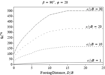
0 50 100 150 200 250 300 350 400 450 500

0 10 20 30

p

γB

β₌90˚, φ₌20

Strength Ratio,c_∕γB

D_∕B₌0

D_∕B₌1

D_∕B₌2

D_∕B₌3

D_∕B₌10₋25

D_∕B₌4

D_∕B₌5

D_∕B₌6

D_∕B₌8

Figure 4.1: Increasing bearing capacity with increased strength ratio

4.2 Effect of Dimensionless Strength Ratio, , continued

4.2.1 Comparison With Footing Distance Ratio

0 50 100 150 200 250 300 350 400 450 500

0 10 20 30

p

γB

β₌90˚, φ₌20

Strength Ratio,c_∕γB

D_∕B₌0

D_∕B₌1

D_∕B₌2

D_∕B₌3

D_∕B₌6₋25

D_∕B₌4

D_∕B₌5

Figure 4.2: Effect of dimensionless strength ratio with footing distance ratio

4.2 Effect of Dimensionless Strength Ratio, , continued

c∕γB=1

c_∕γB₌10

c_∕γB₌20

c_∕γB₌30

β

=

90˚,

H

∕

B

=

4,

φ

=

20˚

c∕γB=30

c∕γB=20

c∕γB=10

c_∕γB₌1

D_∕B₌1 D_∕B₌8

Figure 4.3: Contour plots for dimensionless strength ratio with varied footing distance ratio

4.2 Effect of Dimensionless Strength Ratio, , continued

4.2.2 Comparison With Slope Height Ratio

0 50 100 150 200 250 300 350 400 450 500 550 600

0 10 20 30

p

γB

Strength Ratio,c_∕γB

β₌90˚, D_∕B₌2, φ₌20˚

H_∕B₌0

H_∕B₌1

H_∕B₌2

H_∕B₌3₋16

Figure 4.4: Effect of dimensionless strength ratio with slope height ratio

4.2 Effect of Dimensionless Strength Ratio, , continued

β

=

90˚,

D

∕

B

=

1,

φ

=

20˚

H_∕B₌8

c_∕γB₌1

c∕γB=10

c∕γB=30

c∕γB=20 H_∕B₌1

c_∕γB₌1

c_∕γB₌10

c∕γB=20

c_∕γB₌30

Figure 4.5: Contour plots for dimensionless strength ratio with varied slope height ratio

4.2 Effect of Dimensionless Strength Ratio, , continued

failure planes that have occurred for a slope of the same dimensions even with different strength soils.

4.2.3 Comparison With Friction Angle

0 150 300 450 600 750 900 1050 1200 1350 1500

0 10 20 30

p

γB

Strength Ratio,c_∕γB

β₌90˚, H_∕B₌1, D_∕B₌1

φ₌10˚ φ₌20˚ φ₌30˚ φ₌40˚

Figure 4.6: Effect of dimensionless strength ratio with friction angle

4.2 Effect of Dimensionless Strength Ratio, , continued

β

=

90˚,

H

∕

B

=

2,

D

∕

B

=

1

φ₌10˚ φ₌40˚

c∕γB=1 c∕γB=1

c∕γB=10

c∕γB=10

c_∕γB₌20

c_∕γB₌30 c_∕γB₌30

c_∕γB₌20

Figure 4.7: Contour plots for dimensionless strength ratio with varied internal friction

4.2 Effect of Dimensionless Strength Ratio, , continued

4.2.4 Conclusion

The purpose of this sub--section was to make clear the effect dimensionless strength ratio has on normalised bearing capacity. The assumed knowledge that a higher dimensionless strength ratio will produce a higher bearing capacity has been proven by comparing it against all the main parameters that have an effect of the ultimate bearing capacity of a slope. From the results shown we know that there will be larger differences in bearing capacities between each strength ratio when the slope is stable-- that is either below toe failure or flat ground behaviour-- and that once the slope becomes unstable this difference becomes lessened. From the contour plots we have also gathered that dimensionless strength ratio does not have a noteworthy effect on the failure surface that occurs.

4.3 Effect of Internal Friction Angle,

φ

The friction angle of a soil relates to the shape of each particle that makes up the foundation material. The magnitude of the friction angle of a soil is also a key parameter when determining the bearing capacity of a slope, along with its strength ratio.

The internal friction angle of soil is what determines the amount of material that will be involved in supporting a footing as it affects the interference of one particle on another. A material with zero or extremely low internal friction, such as clay, means each particle is perfectly round or close to it so the particles are unable to stack up on each other, similar to how it is hard to stack a group of basketballs on top of each other due to their round shape. A material with a large friction angle however, such as sand, will stack on top of itself due to the irregularity of each particle binding on adjacent particles.

4.3 Effect of Internal Friction Angle, , continued

4.3.1 Comparison With Dimensionless Strength Ratio

0 150 300 450 600 750 900 1050 1200 1350 1500

10 20 30 40

p

γB

Friction Angle,φ

β₌90˚, H_∕B₌1, D_∕B₌1

c_∕γB₌1

c_∕γB₌10

c_∕γB₌20

c_∕γB₌30

Figure 4.8: Effect of friction angle with dimensionless strength ratio

4.3 Effect of Internal Friction Angle, , continued

β

=

90˚,

H

∕

B

=

4,

D

∕

B

=

4

φ=10˚

c∕γB=1 c∕γB=30

φ=20˚

φ₌30˚

φ=40˚

φ₌10˚

φ₌20˚

φ=30˚

φ=40˚

Figure 4.9: Contour plots for friction angle with varied dimensionless strength ratio

4.3 Effect of Internal Friction Angle, , continued

4.3.2 Comparison With Footing Distance Ratio

0 150 300 450 600 750 900 1050 1200 1350 1500 1650 1800

10 20 30 40

p

γB

Friction Angle,φ

β₌90˚, H_∕B₌2, c_∕γB₌20

D_∕B₌1

D_∕B₌0

D_∕B₌2

D_∕B₌3

D_∕B₌4

D_∕B₌5

D_∕B₌6

D_∕B₌15

D_∕B₌8

D_∕B₌10

D_∕B₌20, 25

Figure 4.10: Effect of friction angle with footing distance ratio

Figure 4.10 again confirms that increasing friction angle ratio increases the bearing capacity of a slope by. We can see the differences in bearing capacity become more noticeable with a higher friction angle as more slope material becomes available to provide resistance to the footing force. We can also again see that the results converge with a smaller friction angle as there will not be as much interaction between the soil particles no matter what the footing distance ratio is. A footing situated at D/B = 2 for a material withφ₌40˚

4.3 Effect of Internal Friction Angle, , continued

β

=

90˚,

H

∕

B

=

2,

c

∕

γ

B

=

20

D_∕B₌10

φ=10˚

φ₌20˚

φ₌30˚

φ=40˚

φ=10˚

φ=20˚

φ₌30˚

φ=40˚

D_∕B₌0

Figure 4.11: Contour plots for friction angle with varied footing distance ratio

Figure 4.11 demonstrates the effect friction angle has on the failure plane for a particular slope. We can observe that for friction angles of φ₌10˚and φ₌20˚footing on slope situation occurs for the smaller footing distance ratio and footing on flat ground situation occurs for the large footing distance ratio as expected. However for friction angles of

4.3 Effect of Internal Friction Angle, , continued

4.3.3 Comparison With Slope Height Ratio

0 250 500 750 1000 1250 1500 1750 2000

10 20 30 40

p

γB

Friction Angle,φ

β₌90˚, D_∕B₌3, c_∕γB₌20,

H_∕B₌0

H_∕B₌6₋16

H_∕B₌1

H_∕B₌2

H_∕B₌3

H_∕B₌4

H_∕B₌5

Figure 4.12: Effect of friction angle with slope height ratio

4.3 Effect of Internal Friction Angle, , continued

β

=

90˚,

D

∕

B

=

3,

c

∕

γ

B

=

20

φ₌10˚

φ=20˚

φ₌30˚

φ₌40˚

φ₌10˚

φ=20˚

φ=30˚

φ₌40˚

H_∕B₌2 H_∕B₌13

Figure 4.13: Contour plots for friction angle with varied slope height ratio

4.3 Effect of Internal Friction Angle, , continued

4.3.4 Conclusion

From the results analysed it has been determined that friction angle does have a large effect on the normalised bearing capacity of a slope. In each of the comparisons that were made the higher friction angles always produced the higher bearing capacities. In the contour plots shown we can see that this higher bearing capacity is due to the increased mass of material that is involved for a higher friction angled material in supporting the footing load. It could be concluded then that for a material with very low friction angle a change in any of the other main parameters would only result in a marginal increase in bearing capacity, and the best material for construction purposes is one with a high friction angle as it will always produce a higher bearing capacity.

4.4 Effect of Footing Distance Ratio,

D

∕

B

Footing distance ratio refers to the distance from the edge of the slope to the face of the footing and is relative to the footing width. This ratio is important to slope analysis as it is a key factor that affects whether a footing is judged as a footing on slope problem or a footing on flat ground problem. This is because as the footing moves away from the slope edge, the instability that may be associated with a particular slope plays a lesser role in the bearing capacity of the slope.

4.4 Effect of Footing Distance Ratio, , continued

4.4.1 Comparison With Dimensionless Strength Ratio

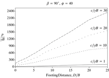
0 60 120 180 240 300 360 420 480 540

0 5 10 15 20 25

p

γB

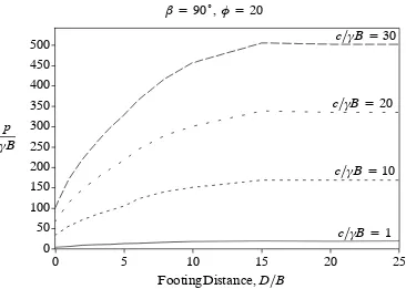
β₌90˚, H_∕B₌4, φ₌20

c_∕γB₌30

c_∕γB₌20

c_∕γB₌10

c_∕γB₌1

FootingDistance,D_∕B

Figure 4.14: Effect of footing distance ratio with dimensionless strength ratio

4.4 Effect of Footing Distance Ratio, , continued

β

=

90˚,

H

∕

B

=

2,

φ

=

20˚

D∕B=1

D_∕B₌3

D∕B=5

D∕B=8

D_∕B₌1

D_∕B₌3

D∕B=5

D∕B=8

c_∕γB₌1 c_∕γB₌30

Figure 4.15: Contour plots for footing distance ratio with varied dimensionless strength ratio

4.4 Effect of Footing Distance Ratio, , continued

4.4.2 Comparison With Slope Height Ratio

0 40 80 120 160 200

0 5 10 15 20 25 30

p

γB

Footing Distance,D_∕B

β₌90˚, c_∕γB₌20, φ₌10˚

H_∕B₌0

H_∕B₌1₋16

H_∕B₌1

H_∕B₌2

H_∕B₌3₋16

Figure 4.16: Effect of footing distance ratio with slope height ratio

4.4 Effect of Footing Distance Ratio, , continued

β

=

90˚,

c

∕

γ

B

=

30,

φ

=

20˚

D∕B=1

D∕B=3

D∕B=5

D_∕B₌8 H_∕B₌2

D∕B=1

D_∕B₌3

D∕B=5

D_∕B₌8

D_∕B₌15 H_∕B₌8

Figure 4.17: Contour plots for footing distance ratio with varied slope height ratio

4.4 Effect of Footing Distance Ratio, , continued

footing distance ratio has failed through to the slope face. For all the other cases for H/B = 8 the failure surfaces are on the verge of failing through the slope face but it didn’t eventuate which could be attributed to the larger soil mass of the slope. We can also see that for the higher slope height ratio flat ground behaviour is not experienced until D/B = 15 while for the lower slope height it occurs at D/B = 8.

4.4.3 Comparison With Friction Angle

0 200 400 600 800 1000 1200 1400 1600 1800

0 5 10 15 20 25

p

γB

Footing Distance,D_∕B

β₌90˚, H_∕B₌2, c_∕γB₌20

φ₌10

φ₌20

φ₌30

φ₌40

Figure 4.18: Effect of footing distance ratio with friction angle

4.4 Effect of Footing Distance Ratio, , continued

β

=

90˚,

H

∕

B

=

2,

c

∕

γ

B

=

20

D_∕B₌1