A hybrid particle swarm evolutionary algorithm for constrained multi-objective optimization

A HYBRID PARTICLE SWARM EVOLUTIONARY

ALGORITHM FOR CONSTRAINED

MULTI-OBJECTIVE OPTIMIZATION

Jingxuan

Wei

School of Computer Science and Technology Xidian University, Xi’an 710071, China &

Department of Maths and Computing

University of Southern Queensland, Australia

e-mail:[email protected]

Yuping

Wang

School of Computer Science and Technology Xidian University, Xi’an 710071, China

Hua

Wang

Department of Maths and Computing

University of Southern Queensland, Australia

Manuscript received 17 March 2008; revised 19 August 2008 Communicated by Vladim´ır Kvasniˇcka

for bi-objective optimization problems. It can assign larger crowding distance func-tion values not only for the particles located in the sparse region but also for the particles located near to the boundary of the Pareto front. In this step, the reference points are given, and the particles which are near to the reference points are kept no matter how crowded these points are. Thirdly, a new mutation operator with two phases is proposed. In the first phase, the total force is computed first, then it is used as a mutation direction, searching along this direction, better particles will be found. The comparative study shows the proposed algorithm can generate widely spread and uniformly distributed solutions on the entire Pareto front.

Keywords: Conostrained multi-objective optimization, particle swarm optimiza-tion, evolutionary algorithm

1 INTRODUCTION

In general, many real-world applications involve complex optimization problems with variants competing specifications and constraints. Without loss of generality, we consider a minimization problem with decision space S, which is described as follows:

  

 

minx∈S f(x) ={f1(x), f2(x), . . . , fm(x)}

s.t. gj(x)≤0, j= 1,2, . . . , s

hj(x) = 0, j= 1,2, . . . , p,

(1)

where x = (x1, x2, . . . , xn) is the decision vector, S is an n-dimensional

rectan-gle space defined by the parametric constraintslk ≤ xk ≤ uk, k = 1,2, . . . n. In

constrained multi-objective optimization problems, all equality constraints can be converted to inequality constraints by |hj(x)| ≤ ε, whereε is a small value. This

allows us to deal with only the inequality constraints. Constraint violation is defined as Φ(x) =Ps+p

j=1max(0, gj(x)). f1, f2, . . . , fmaremobjectives to be minimized. The

aim of the constrained multi-objective optimization problems (constrained MOPs) is to find multiple nondominated solutions under constraints. If these nondominated solutions are uniformly distributed and widely spread along the Pareto front, their quality is better.

Constraint handling is a crucial part of real-world problem solving and it is time that MOEA researchers focus on solving constrained MOPs [9].

One of the typically algorithms to solve constrained MOPs is NSGAII with constraint dominance principle [7], which allow each feasible solution has a better rank than any infeasible one. Obviously, the main drawback of this principle is that the algorithm probably results in the premature convergence. In order to overcome the problem, some relevant algorithms are proposed [10, 11]. In these problems, the infeasible solutions which are located near to the boundary of the feasible region and have small rank values are kept during the evolution. But the infeasible solutions with larger constraint violations and smaller rank values are not concerned. In fact, these solutions may be valuable for finding the true Pareto front. So we design two new infeasible particle preservation strategies in Section 3.

Particle swarm optimization (PSO) [12, 13] is a relatively recent heuristic in-spired by the choreography of a bird flock. PSO seems suitable for the multi-objective optimization mainly because of the high speed of convergence that the al-gorithm presents for single-objective optimization. However, such convergence speed may be harmful in the context of multi-objective optimization, because a PSO-based algorithm may converge to a false Pareto front. In order to overcome this drawback, some PSO algorithms incorporate a mutation operator which can enriches the ex-ploratory capabilities of algorithms [14, 15].

In recent years, the field of MOPSO has been steadily gaining attention from re-search community [16–19]. While PSO is rarely considered in constrained MOPs [20].

simulations for five constrained MOPs are made. The performances of the proposed algorithm are compared with that of NSGAII and MOPSO. The results indicate that the proposed algorithm has better performances for the test functions, especially for the problems with two or more disconnected feasible regions.

2 PRELIMINARIES

2.1 Particle Swarm Optimization

PSO has been developed by Kennedy and Eberhart [12, 13]. The original PSO formulae are:

Vi(t+ 1) =ωVi(t) +c1rand1(pbesti(t)−xi(t)) +c2rand2(gbest(t)−xi(t)) (2)

xi(t+ 1) =xi(t) +Vi(t+ 1), i= 1,2, . . . ,popsize. (3)

In essence, the trajectory of each particle is updated according to its own best position pbest , and the best position of the whole swarm denoted as gbest. Vi =

(Vi1, Vi2, . . . , Vin) represents the velocity of the ith particle, and theith particle is

denoted as an-dimensional vectorxi= (xi1, xi2, . . . xin), namely the position of the

ith_{particle isx}

i, and every particle represents a potential solution. rand1andrand2

are two random values obeying uniform distribution in [0,1]. c1 is the cognition

weight andc2 is the social weight. popsize is the size of the swarm.

2.2 Constrained MOPs

Definition 1. For the multi-objective optimization, a vectorµ = (µ1, µ2, . . . , µn)

is said to dominate a vector ν = (ν1, ν1, . . . , νn) (denoted as µ ≺ ν) if: ∀i ∈

{1,2, . . . , m}, fi(µ)< fi(ν)∧∃j ∈ {1,2, . . . , m}, fj(µ)< fj(ν). A solutionx ∈S

is called a Pareto-optimal solution for problem (1), if Φ(x) = 0 and ∼ ∃−→x ∈ S such that Φ(−→x) = 0 and~x≺x. All optimal solutions constitute the Pareto-optimal set. The corresponding set in the objective space is called Pareto front.

3 THE PRESERVATION STRATEGIES OF THE PARTICLES

3.1 The New Comparison Strategy in Particle Swarm Optimization

In order to keep some particles with smaller constraint violations, a new comparison strategy is proposed. Firstly, a threshold value is proposed: ψ = 1

T

Ppopsize

i=1 Φ(xi)/

popsize, T is a parameter, which decreases from 0.4-0.8 with the increasing of the generation number. In every generation, if the constraint violation of a particle is less than the threshold value, the particle is acceptable, else it is unacceptable. The comparison strategy is described as follows:

1. If two particles are feasible solutions, we select the one with the smaller rank values.

2. If two particles are infeasible, we select the one with the smaller constraint violation.

3. If one is feasible and the other is infeasible, if the constraint violation of the infeasible one is smaller than the threshold value and it is not dominated by the feasible one, we select the infeasible one.

3.2 Infeasible Elitist Preservation Strategy

In order to keep some particles with smaller rank values, some infeasible solutions beside the feasible ones should be kept to act as a bridge connecting two or more feasible regions during optimization. The procedure of the process of keeping and updating infeasible elitists is given by Algorithm 1. Let R denotes the Pareto-optimal set found so far, IR denotes the infeasible elitist set, and SI denotes the size of the infeasible elitist set. SR denotes the size ofR.

Algorithm 1. Step 1: For every infeasible particle in the swarm, if it is not do-minated by any other particle in the setR, add it to IR.

Step 2: Remove particles in IR which are dominated by any other member ofR.

Step 3: If the size of the IR exceeds the given maximum number SI, then do:

1. select SI particles in IR with smaller rank values whent < tmean.

2. select SI particles in IR with smaller constraint violations whent > tmean.

The rank value ofxiis equal to the number of the solutions that dominate it.

tis the current generation number andtmean= tmax₂ ,tmaxis the maximum generation

number. At the early stage of evolution(t < tmean) we need to enlarge the search

domain in order to keep the diversity of the swarm. So the particles of smaller rank values are kept, which will make the swarm converge to the true Pareto front, and at the later stage of evolution (t > tmean), in order to guarantee the convergence of

4 A NOVEL CROWDING DISTANCE FUNCTION

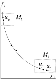
In multi-objective optimization, we have to find a set of solutions which is high competitive in terms of convergence, distribution, and diverse. In section 3, the infeasible elitist preservation strategy and the new comparison strategy make the algorithm have better convergence but can not guarantee the diversity and distri-bution of Pareto-front. In [7, 20], crowded-comparison operator is adopted which guides the search toward a sparse region of Pareto front, but it does not pay more attention to the crowded regions near to the boundary of Pareto front. However, the boundary points (they are also called reference points) can guarantee the diversity of the Pareto-front, some particles located near to the boundary of the Pareto front are of important information. In this part, for the two-objective optimization, we design a novel crowding distance function denoted as crowd(x), which assigns larger function values not only for the solutions located in a sparse region, but also for the solutions located in a crowded region near to the boundary of the Pareto front.

The procedure is given by Algorithm 2. Suppose that the current Pareto front is composed of N points, denoted as M ={u1, u2, . . . , uN}, and the corresponding

points in the decision space are denoted asx1, x2, . . . , xN, let ub, uc be two

refer-ence points of the Pareto front (can be seen from Figure 1), and the corresponding points in the decision space be xb, xc. xb = arg min{f2(x1), f2(x2), . . . , f2(xN)},

xc=argmin{f1(x1), f1(x2), . . . , f1(xN)}.

Algorithm 2. Step 1: Calculate the Euclidean distance between every point in the Pareto front and ub, find region M1 which is near to the boundary of the

Pareto front:

Di1= dist(ui, ub), i= 1,2, . . . , N

D1=

N

X

i=1

Di1

1 N

M1={uj |dist(uj, ub)≤0.5D1,1≤j≤N, uj 6=ub}.

Step 2: Calculate the Euclidean distance between every point in the setM/M1and

uc, find regionM2which is near to the reference point:

Di2= dist(ui, uc), ui∈M/M1

D2=

|M/M1| X

i=1

Di2

1 |M/M1|

Step 3: Calculate the crowding distance of every point in the Pareto front:

crowd(xi) =

      

     

crowd1(xi)·_dist(dist(u_ubb,u,uci)), ui∈M1 crowd1(xi)·_dist(dist(u_ubc,u,uci)), ui∈M2 crowd1(xi)· dist(ub,u

c)

min{amin,bmin}, ui=uborui=uc

crowd1(xi), else

(4)

where amin = min{dist(ub, ui)|ui ∈ M1}, bmin = min{dist(ub, ui)|ui ∈ M2},

crowd1 = D1+₂D2, D1, D2 are two nearest distances between point ui and the

other points in the Pareto front.

1

M

2

M

b

u

i

u

c

u

1

f

2

f

Fig. 1. Crowding distance calculation

In doing so, when the Pareto optimal solutions exceed the given number, we keep these particles with larger crowding distance function values, namely the particles located in the sparse region of the objective or near to the boundary of the Pareto font are preserved. So finally, we will get a widely spread and uniformly distributed Pareto front.

5 USE OF A NOVEL MUTATION OPERATOR

In PSO, the search scheme is singleness: every particle is updated only according to its own best position as well as the best particle in the swarm. So it often results in two outcomes:

1. the loss of diversity required to maintain a diverse pareto front; 2. premature convergence if the swarm is trapped into a local optima.

section, a novel mutation operator with two phases is proposed. The aim of the first phase is to make full use of all particles in the swarm, and define a mutation direction. Searching along this direction, better new particles will be found. In order to make particles search different regions, which can guarantee the convergence of the algorithm, the second phase of mutation is proposed.

More details are described as follows:

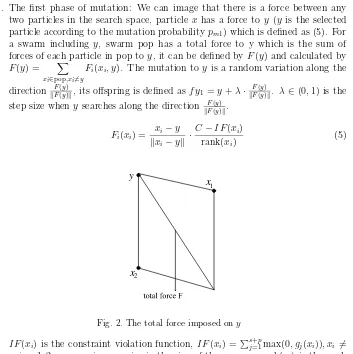
1. The first phase of mutation: We can image that there is a force between any two particles in the search space, particlex has a force to y (y is the selected particle according to the mutation probabilitypm1) which is defined as (5). For

a swarm including y, swarm pop has a total force to y which is the sum of forces of each particle in pop toy, it can be defined byF(y) and calculated by F(y) = X

xi∈pop,xi6=y

Fi(xi, y). The mutation toy is a random variation along the

direction _kFF(_(yy)_)k, its offspring is defined asf y1 =y+λ·_kF_F(₍y_y)_)k. λ∈(0,1) is the

step size whenysearches along the direction _kF_F(₍y_y)_)k.

Fi(xi) =

xi−y

kxi−yk

·C−IF(xi) rank(xi)

(5)

1

x

2

x

y

Fig. 2. The total force imposed ony

IF(xi) is the constraint violation function, IF(xi) =

Ps+p

j=1max(0, gj(xi)), xi6=

y, i = 1,2, . . . ,popsize, popsize is the size of the swarm. rank(xi) is the rank

value ofxiin the current swarm. C is a big constant, letC= 10 000. This can

be graphically illustrated by Figure 2.

From Figure 2 and Equation (5), we can see that the total force imposed ony leans to the particle with lower constraint violation or smaller rank value. So searching along this direction, better particles may be found.

of mutation is performed: for f y1 (f y1 is selected according to the second

mutation probability pm2, we divide the ith interval [li, ui] into n

subinter-vals [̟i

1, ̟i2], . . . ,[̟n

i−1

i , ̟n

i

i ], where |̟ij −̟ji−1| < ε, j = 2, . . . ni, randomly

generate a number δ ∈ (0,1); if δ < pm2, then randomly select one ̟ji in

{̟i

1, ̟i2, . . . , ̟ini}as the value of thei

th_dimension.

6 THE PROPOSED ALGORITHM

Algorithm 3(Hybrid particle swarm evolutionary algorithm: HPSEA).

Step 1: Choose the proper parameters, given swarm size popsize, randomly gene-rate initial swarm pop(0) including every particle’s position and velocity, find the Pareto optimal solutions in the current swarm and copy them to R. Let t= 0.

Step 2: Preserve infeasible elitist set IR according to Section 3.

Step 3: For every particle, let pbesti=xi, i= 1,2, . . . ,popsize.

Step 4: Select the best position of the swarm asgbest,gbestis randomly selected from setR.

Step 5: For every particle in the swarm, do:

1. If rand(0,1)< pc, pc = 0.2 +e−(

t

tmax+1), pbest

i is selected randomly from

the set IR, else pbest_iis unchangeable.

2. The position and velocity ofxiare updated according to (2), (3). The new

swarm is denoted as pop(t+ 1).

Step 6: For every particle in pop(t+ 1), use mutation operator in Section 5 and get the swarm pop(t+ 1).

Step 7: Maintain the particles in pop(t+1) within the search space: when a decision vector goes beyond its boundaries, then the decision vector takes the value of its corresponding boundary.

Step 8: Update the setRwith all particles in pop(t+ 1), the update means adding all Pareto optimal solutions in pop(t+ 1) intoR, and delete the dominated ones in it.

If the size ofRis full, the predetermined number of particles with larger crowding distance function values are preserved.

Step 9: Update the infeasible elitist set IR with all particles in pop(t+1) according to the infeasible elitist preservation strategy in Section 3.2.

Step 10: For every particlexi, update its pbestiaccording to the new comparison

strategy in 3.1.

In step 5, when rand(0,1)< pc, we choose the pbest from the set IR; in doing

so, a particle’s potential search space will be enlarged, wherepc= 0.2 +e−(

t tmax+1)

means the value is dynamically changed with the current generation numbert. It means at the beginning of the search, in order to enlarge the potential search space and keep diversity of the swarm, a larger number of infeasible solutions are selected while at the later stage of evolution, in order to guarantee the convergence of the swarm, a smaller number of infeasible solutions are kept. So the infeasible elitists must be in a proper proportion, in this paperpc∈[0.335,0.561].

7 THE PROPOSED ALGORITHM

7.1 Test Functions

There are five test problems from the literature in our experiments. TheF1 ∼F4

are chosen from [9],F5is chosen from [7]. The above test problems provide difficulty

to an algorithm in the vicinity of the Pareto front; difficulties also come from the infeasible search regions in the entire search space.

F1 :

        

minf1(x) =x1

minf2(x) =c(x) exp(−f1(x)/c(x))

s.t. g1(x) =f2(x)−0.858 exp(−0.541f1(x))≥0

s.t. g2(x) =f2(x)−0.728 exp(−0.295f1(x))≥0

x= (x1, x2, . . . , x5), 0≤x1≤1,−5≤xi≤5, i= 2,3,4,5.

F2∼F4:           

minf1(x) =x1

minf2(x) =c(x)(1−f_c1₍(_xx₎))

s.t. g1(x) = cos(θ)(f2(x)−e)−sin(θ)f1(x)≥

a|sin(bπ(sin(θ)(f2(x)−e) + cos(θ)f1(x))c)|d

x= (x1, x2, . . . , x5), 0 ≤x1 ≤1, −5≤xi≤5, i= 2,3,4,5, parameter settings are

described in Table 1. ForF1∼F4,c(x) = 41 +P5i=2(x2i−10 cos(2πxi)).

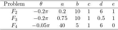
Problem θ a b c d e

F2 −0.2π 0.2 10 1 6 1

F3 −0.2π 0.75 10 1 0.5 1

F₄ −0.05π 40 5 1 6 0

Table 1. Parameter settings inF2∼F4

F5:         

minf1(x) =x1

minf2(x) = (1 +x2)/x1

s.t. g1(x) =x2+ 9x1≥6

s.t. g2(x) =−x2+ 9x1≥1

7.2 Parameter Values

Each simulation run was carried out using the following parameters: swarm size: 100; infeasible elitist size: 20; size ofR: 100; mutation probabilitypm1 : 0.6, pm2=

0.3; maximum number of generationstmax: 200,c1 =c2 = 0.8; ωmax= 1.0, ωmin=

0.4.

7.3 Performance Measures

In the following of this section letA,Brepresent two sets of Pareto optimal solutions in the decision space, andP A,P B denote the corresponding Pareto solution sets in the objective space. We propose three metrics to measure the quality, distribution, and diverse of the Pareto front. The first metric known as Q-measure [21] is used to compare the quality of solutions found by the two algorithms. The second known as S-measure [22] is used to evaluate the uniformity of the Pareto optimal solutions. The third known as the FS-measure [23] is used to measure the size of the space covered by the Pareto front found by an algorithm.

Metric 1 (Q-measure). Let Φ be the nondominated solution set ofA∪B, let Ψ = Φ∩A, Θ = Φ∩B, the metric is defined byM1(A, B) = _||_ΦΨ_||,M1(B, A) = |_|Θ_Φ|_|. The

solution set P Ahas better convergence to the true Pareto front than the solution setP B, if and only ifM1(A, B)> M1(B, A) orM1(A, B)>0.5.

Metric 2 (Metric two (S-measure)). S= [ 1

nP F

PnP F

i=1(d ′

i−d

′₎2_]1/2_,d′₌ 1

nP F

PnP F

i=1 d ′

i,

wherenP Fis the number of the solutions in the known Pareto front,d′iis the distance

(in the objective space) between the numberiand its nearest member in the known Pareto front. The smaller the value of S-measure, the more uniformity the Pareto front found by the algorithm will be.

Metric 3 (Metric three (FS-measure)).

F S = qPm

i=1min(x0,x1)∈A×A{(fi(x0)−fi(x1))

2_{}, the larger the value of F S is, the}

better diverse of solutions on the Pareto front will be.

7.4 Simulation Results and Comparisons

0.48 0.49 0.5 0.51 0.52 0.53 0.54 0.55 0.56 0.57 0.58

Q−measure

M1(1,2) M1(1,3) M1(2,3) 1 2 3

2 3 4 5 6 7 8

x 10−3

S−measure

1 2 3

0.4 0.5 0.6 0.7 0.8 0.9 1 1.1

FS−measure

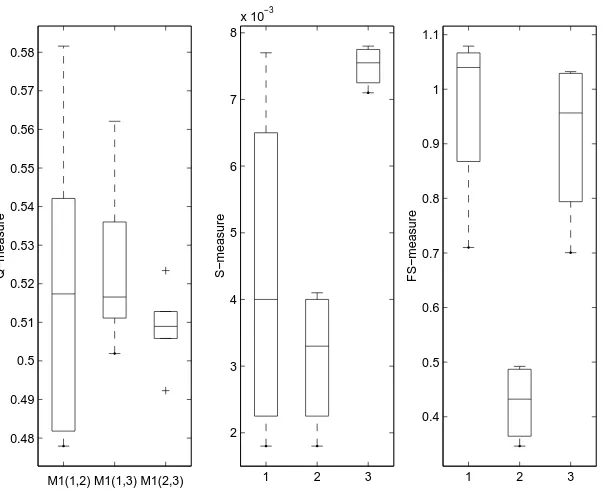
Fig. 3. Statistical performance onF1

A. F1

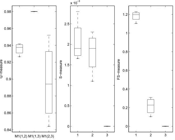
0.84 0.86 0.88 0.9 0.92 0.94 0.96 0.98

M1(1,2) M1(1,3) M1(2,3)

Q−measure

1 2 3

0 0.5 1 1.5 2 2.5

x 10−3

S−measure

1 2 3

0 0.2 0.4 0.6 0.8 1 1.2

FS−measure

Fig. 4. Statistical performance onF2

B. F2

The nature of the constraint boundary ofF2 makes the Pareto optimal region

discontinuous, having a number of disconnected continuous regions. The task of an optimization algorithm would be to find as many such disconnected regions as possible. It can be seen from Figure 4 that HPSEA and CNSGAII are able to find at least part of the true Pareto front, but MPSO can not find a few part of the true Pareto front. It can be observed that HPSEA is able to find a diverse and nearly Pareto optimal front due to the high value of Q-measure and FS-measure. We can also see that the Pareto front found by CNSGAII is more uniform than HPSEA due to the low value of S-measure, but CNSGAII can only find a small part of the true Pareto front. This is because HPSEA adopts two phases infeasible elitist preservation strategies which can maintain diversity of the swarm during optimization, and finally get the true Pareto front. C. F3

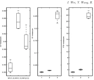
0.52 0.54 0.56 0.58 0.6 0.62 0.64 0.66 0.68

M1(1,2) M1(1,3) M1(2,3)

Q−measure

1 2 3

0.05 0.1 0.15 0.2 0.25

S−measure

1 2 3

4 6 8 10 12 14 16 18 20 22 24

FS−measure

Fig. 5. Statistical performance onF3

Pareto-front. Although MPSO maintains a better spread of solutions in terms of the high value of FS-measure in Figure 5, HPSEA is able to come closer to the true Pareto-front due to the high value of Q-measure. Algorithms which tend to converge anywhere in the Pareo front first and then work on finding a spread of solutions will end up finding solutions. HPSEA shows a similar behavior in this problem.

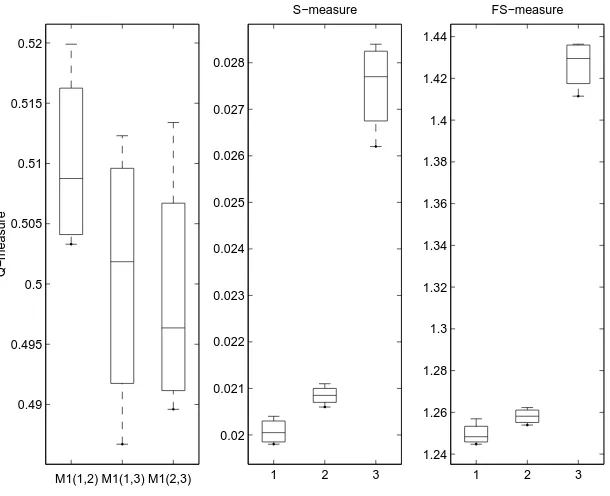
D. F4

0.49 0.495 0.5 0.505 0.51 0.515 0.52

M1(1,2) M1(1,3) M1(2,3)

Q−measure

1 2 3

0.02 0.021 0.022 0.023 0.024 0.025 0.026 0.027 0.028

S−measure

1 2 3

1.24 1.26 1.28 1.3 1.32 1.34 1.36 1.38 1.4 1.42 1.44

FS−measure

Fig. 6. Statistical performance onF4

E. F5

For the problemF5, HPSEA have better convergence to the true Pareto front

due to the high value of Q-measure. The Pareto front found by NSGAII is more uniform due to the low value of S-measure and MPSO finds a wider spread Pareto front due to the higher value of FS-measure.

Finally, we can conclude that for F1, F2, HPSEA performs best in terms of

convergence and diversity, and for F3, F4, HPSEA performs best in terms of

con-vergence and uniformity. For F5, IPSEA performs best in terms of convergence,

MPSO performs best in terms of diversity and CNSGAII performs best in terms of uniformity.

8 CONCLUSIONS

0.5 0.51 0.52 0.53 0.54 0.55 0.56

Q−measure

M1(1,2),M1(1,3),M1(2,3) 1 2 3

0.04 0.06 0.08 0.1 0.12 0.14 0.16 0.18 0.2 0.22

S−measure

1 2 3

7.3 7.4 7.5 7.6 7.7 7.8 7.9 8

FS−measure

Fig. 7. Statistical performance onF5

front. Compared to the other algorithms, the proposed algorithm is superior to these algorithms.

Acknowledgement

This research is supported by National Natural Science Foundation of China (No. 60-873099).

REFERENCES

[1] Hajela, P.—Lin, C. Y.: Genetic Search Strategies in Multicriterion Optimal

De-sign. Structural Optimization, Vol. 11, 1992, No. 5, pp. 99–107.

[2] Fonseca, C. M.—Fleming, P. J.: Genetic Algorithms for Multiobjective

Opti-mization: Formulation, Discussion and Generalization. In: S. Forrest, et al. (Eds.): Proc. 5th_{Inter. Conf. Genetic Algorithms, San Mateo, California, Morgan Kaufman,}

1993, pp. 416–423.

[3] Horn, J. N.—Goldberg, D. E.: A Niched Pareto Genetic Algorithm for

Multiob-jective Optimization. In: N. Nafpliotis, et al. (Eds.): Proc. 1st _{IEEE Conf.}

[4] Srinivas, N.—Deb, K.: Multobjective Optimization Using Nondominated Sorting in Genetic Algorithms. Evolutionary Computation, Vol. 2, 1994, No. 3, pp. 221–248.

[5] Knowles, J. D.—Corne, D. W.: Approximating the Nondominated Front Using

The Pareto Archived Evolutionary Strategy. Evolutionary Computation, Vol. 8, 2000, pp. 149–172.

[6] Coello, C. A.—Pulido, G. T.: Multiobjective Optimization Using A

Micro-genetic Algorithm. In: L. Spector, et al. (Eds.): Proc. Genetic and Evolutionary Computation Conf. (CEC ’2002). Honolulu, HI, 2002, pp. 1051–1056.

[7] Deb, K.—Pratap, A.—Agarwal, S.—Meyarivan, T.: A Fast and Elitist

Mul-tiobjective Genetic Algorithm: NSGAII. IEEE Transactions on Evolutionary Com-putation, Vol. 6, 2002, No. 2, pp. 182–196.

[8] Zitzler, E.—Laumanns, M.—Thiele, L.: Improving the Strength Pareto

Evolu-tionary Algorithm [R]. Zurich. 2001.

[9] Deb, K.—Pratap, A.—Meyarivan, T.: Spea 2: Constrained Test Problems for

Multiobjective Evolutionary Optimization [R]. KanGAl Report No. 200002.

[10] Cai, Z.—Wang, Y.: A Multiobjective Optimization-based Evolutionary Algorithm

for Constrained Optimization. IEEE Transactions on Evolutionary Computation, Vol. 10, 2006, No. 6, pp. 658–663.

[11] Zhou, Y.—He, J.: A Runtime Analysis of Evolutionary Algorithms for Constrained

Optimization Problems. IEEE Transactions on Evolutionary Computation, Vol. 11, 2007, No. 5, pp. 608–619.

[12] Kennedy, J.—Eberhart, R.: Particle Swarm Optimization. In Proceedings of the

IEEE International Conference on Neural Networks. IEEE Service Center, Piscat-away, NJ, IV, 1995, pp. 1941–1948.

[13] Kennedy, J.—Eberhart, R.—Shi, Y.: Swarm Intelligence: SanFrancisco:

Mor-gan Kaufmann Publishers. 2001.

[14] Xie, X.—Zhang, F.: A Dissipative Particle Swarm Optimization. Proc. of the

IEEE Int. Conf. on Evolutionary Computation. IEEE Service Center, Piscataway, 2002, pp. 1666–1670.

[15] Eberhart, R. C.—Kennedy, J.: A New Optimizer Using Particle Swarm Theory.

The 6thInt. Symp. on Micro Machine and Human Science. Nagoya, 1995, pp. 39–43.

[16] Coello, C.—Lechunga, M.: MOPSO: A Proposal for Multiple Objective Particle

Swarm Optimization. In Proc. of the 2002 Congress on Evolutionary Computation. IEEE Service Center, Piscataway, 2002, pp. 1051–1056.

[17] Li, X.: A Nondominated Sorting Particle Swarm Optimizer for Multiobjective

Op-timization: Formulation, Discussion and Generalization. In: E. Cantu-Paz, et al. (Eds.): Proc. Genetic and Evolutionary Computation, GECCO, Springer-Verlag, Berlin, 2003, pp. 37–48.

[18] Parsopoulos, K.—Vrahatis, M.: Particle Swarm Optimization Method in

Mul-tiobjective Problems. In Proc. 2002 ACM Symp. Applied Computing. Madrid, Spain, 2002, pp. 603–607.

[19] Fieldsend, J.—Sing, S.: A Multi-Objective Algorithm Based Upon Particle Swarm

[20] Coello, C. A.—Toscano Pulido, G.: Handling Multiple Objectives with Particle Swarm Optimization. IEEE Trans on Evolutionary Computation, Vol. 8, 2004, No. 3, pp. 205–230.

[21] Wang, Y.—Dang, Ch.: Improving Multiobjective Evolutionary Algorithm by

Adaptive Fitness and Space Division, ICNC ’05, Springer-Verlag, Berlin. Changsha, China, 2005, pp. 392–398.

[22] Shaw, K. J. A.—Notcliffe, L.: Assessing the Performance of Multiobjective

Ge-netic Algorithms for Optimization of Batch Process Scheduling Problem. In Proc. Conf. Evol. Comput. UK, 1999, pp. 37–45.

[23] Bosman Thierens, P. D.: The Balance Between Proximity and Diversity in

Mul-tiobjective Evolutionary Algorithms. IEEE Trans on Evolutionary Computation, Vol. 7, 2003, No. 2, pp. 174–188.

Jingxuan Weireceived Ph. D. degree in applied mathematics from Xidian University, Xi’an, China. She is a lecturer at Xidian University. Her research interests include evolutionary computa-tion, particle swarm optimizacomputa-tion, multi-objective optimization.

YupingWangis a Full Professor at Xidian University, Xi’an, China. He has published more than 40 journal papers. He received the Ph. D. degree in Computational mathematics from Xi’an Jiaotong University, Xi’an, China, in 1993. his current research interests include evolutionary computation and optimization theory, methods and applications, etc.