Conceptualising and interpreting reliability

Conceptualising and interpreting

reliability

Sandra Johnson

Rod Johnson

Ofqual/10/4706

December 2009

This report is the principal outcome of a conceptual analysis project focusing on assessment reliability commissioned by the Office of the Qualifications and Examinations Regulator (Ofqual) in January 2009. As required, the analysis is contextualised with reference to the kinds of tests, examinations and qualifications that are common in the UK.

The specific requirements for the project were to:

 identify different approaches to conceptualising ‘truth’ and ‘error’ within reliability theory – alternative models of reliability

 identify different approaches to estimating reliability, highlighting: o the assumptions that they make

o their basis in models of reliability o their strengths and weaknesses

 consider how best to evaluate estimates of reliability, based on different approaches, given complications such as the following:

o that not all sources of random error are likely to be accounted for o that other (systematic) sources of error will be unaccounted for o that results may be used for a variety of different purposes

The following definition of ‘reliability’ was given:

Reliability refers to the consistency of outcomes that would be observed from an assessment process were it to be repeated. High reliability means that broadly the same outcomes would arise. Unreliability can be attributed to ‘random’,

unsystematic causes of error in assessment results. Given the general parameters and controls that have been established for an assessment process – including test specification, administration conditions, approach to marking, linking design and so on – (un)reliability concerns the impact of the particular details that do happen to vary from one assessment to the next for whatever reason.

A number of individuals helped us with the production of this report. Firstly, we thank Qingping He and members of Ofqual’s reliability programme Technical Advisory Group for extremely useful feedback on the first draft. We also gladly acknowledge the very supportive input that we received from Anton Béguin, Robert Brennan, Jean Cardinet, Dany Laveault, George Marcoulides and Richard Shavelson, who assisted us in identifying relevant publications and who were also willing to share their thoughts about reliability estimation with us. As far as the awarding bodies in the UK are concerned, we are very grateful to the following individuals and their

1 Introduction 1

1.1 Tests, examinations and qualifications in the UK 1

1.2 The nature of educational assessment 2

1.3 Reliability and validity 4

2 The evolution in reliability conceptualisation 8

2.1 Observed scores, true scores and measurement error 8

2.2 True Score Theory 9

2.3 Equivalent tests 12

2.4 Coefficient alpha 13

2.5 Beyond alpha 16

2.6 Item response models 19

2.7 Variance analysis and generalizability 21

3 The variance components model 23

3.1 Generalizability coefficients and standard errors of measurement

23

3.2 Subsuming classical reliability indicators as special cases 25

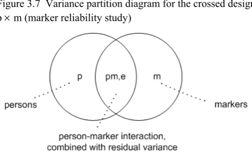
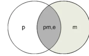
3.3 Marker reliability studies 33

3.4 A comment on ‘hidden’ factors 37

4 Extending variance analysis in reliability estimation 38

4.1 Investigating question and marker effects simultaneously 38

4.2 Taking account of demographics and other grouping characteristics

43

4.3 Assessing reliability at the level of whole examinations 47

5 Reliability estimation and reporting: the way forward? 50

5.1 The need to report on reliability 50

5.2 Reliability as replicability 52

5.3 Researching reliability and acting on findings 54

5.4 A final note on the validity risks for reliability 55

1 Introduction

1.1 Tests, examinations and qualifications in the UK

There are currently over 120 awarding bodies operating in the UK’s market-driven qualifications system, between them offering over 6000 nationally accredited academic and vocational/occupational qualifications (for details see the National Database of Accredited Qualifications: www.accreditedqualifications.org.uk). The system is regulated in England by the Office of the Qualifications and Examinations Regulator (Ofqual), in Wales by the Department for Children, Education, Lifelong Learning and Skills (DCELLS), in Northern Ireland by the Council for the

Curriculum, Examinations and Assessments (CCEA), and in Scotland by the Scottish Qualifications Authority (SQA).

In the academic arena, the principal qualifications for upper secondary school students are the General Certificate of Secondary Education (GCSE), normally taken at the end of Year 11 (16 year olds) and the General Certificate of Education Advanced Level (A level), typically taken as a school leaving examination at the end of Year 13 (18 year olds). These qualifications are currently offered by three awarding bodies in England – the Assessment and Qualifications Alliance (AQA), Edexcel, and Oxford, Cambridge and RSA Examinations (OCR). There is a single awarding body in each of Wales and Northern Ireland, respectively the Welsh Joint Education Committee (WJEC) and the CCEA. In Scotland, the national qualifications system comprises Standard Grade, Highers and Advanced Highers, offered by the SQA. In all countries, qualifications are available in a wide variety of traditional and less traditional subjects, including, for example, history, French, mathematics, business studies, ICT, art and design, citizenship studies, drama, psychology. Examinations are typically modular, with individual units often assessed in different ways within a single examination. Tests might comprise multiple choice questions, delivered on paper or online, structured response questions or essays, or could take the form of a practical test or an oral interaction with an assessor. Course work might also be included in the final performance profile that eventually leads to a grade.

creative and media, hair and beauty studies, science, construction and the built

environment, hospitality, engineering. Generic learning is common across all Diploma Lines of Learning. It includes a core of skills that employers and higher education demand, and requires learners to develop their organisational, research and

presentation skills through completion of a project – for example a performance or written report – in addition to undergoing a minimum of 10 days' work experience. Additional and/or specialist learning gives learners the opportunity to deepen or broaden their learning. The component outcomes – often stand-alone qualifications – are aggregated to form the full Diploma.

Underneath this vast and still growing qualifications system, the National Curriculum assessment programme continues in England. This was introduced into primary and early secondary education in the late 1980s, and is an annual census of pupil

attainment at key stages in the school system. Managed by the Qualifications and Curriculum Development Authority (QCDA), the programme essentially ‘certificates’ every pupil as that pupil progresses through the key stages. The results of the

certification serve multiple purposes, from reporting learning progress to parents and teachers to monitoring the effectiveness of schools, authorities and the national education system as a whole. The programme has undergone a number of evolutions since its introduction, and currently focuses on the assessment of English and

mathematics at the end of Year 2 (Key Stage 1), and English, mathematics and

science at the end of Year 6 (Key Stage 2). At Key Stage 1, and for science attainment at Key Stage 2, pupil attainment is currently assessed through teacher judgement, supported by in-class use of National Curriculum tasks. At Key Stage 2 mathematics attainment is assessed each year using two national pen and paper tests (both taken by each pupil), while English is assessed using a single reading test and two writing assignments, one short and one extended.

This report explores the issue of assessment reliability against this complex reality. The project requirement was to consider different conceptualisations of reliability, interpreting and evaluating these with particular reference to the kinds of tests, examinations and qualifications common in the UK. Questions of interest are:

 How has assessment reliability been conceptualised?

 What are the technical assumptions associated with one or other conceptualisation?

 Are there particular conceptualisations that serve particular assessment purposes

more adequately than others?

 What are the consequences of adopting an inappropriate conceptualisation for investigating and reporting reliability?

Before addressing these questions, let us first remind ourselves why assessment reliability, and indeed assessment validity, is such an issue.

1.2 The nature of educational assessment

questionnaires and product evaluations. And individuals can assess themselves, or be assessed by others, including peers, teachers and external agencies. But what evidence do we look for when we engage in educational assessment? Where do we look for it? How exactly should we gather it, and how will we know when we have enough? The answers to these questions depend very much on the nature of what is being assessed, what the context for assessment is, who is doing the assessment, and why it is being carried out. Why is this apparently simple process so fraught with difficulty?

The defensible assessment of intellectual skills and abilities has always been, and will continue to be, a challenging endeavour, no matter the form of assessment. This is because the skills and abilities that we are trying to measure are often difficult to define in any absolute sense, and cannot be directly observed. It is these properties that distinguish them from more readily measurable physical properties like height and weight. Because they are not directly observable we are constrained to employ a number of different strategies in efforts to elicit observable evidence of their

existence. We pose questions to individuals – questions whose answers provide us with some relevant information about their subject knowledge and ability. Or we give instructions – instructions that require particular observable behaviours to be

deployed, behaviours that tell us something about conceptual understanding or skills development.

The instruments of assessment might be informal task-based exercises conducted during normal class time. Examples would be producing a piece of fictional writing in English, sketching a portrait in art, setting up some laboratory equipment in physics, or crafting a soup ladle in woodwork. Alternatively, they might be conventional tests, timed or untimed, comprising a set of obligatory ‘atomistic’ test items (usually in objective format), a small number of structured or essay questions with choice options, or an oral interaction with peers or an assessor. The test might focus on a particular curriculum topic in depth, or thinly sample the curriculum as a whole. Alternatively, it might involve a lengthy practical demonstration of knowledge and skill. The test might be a stand-alone device, such as a standardised reading test used by teachers in their own classrooms, or a ‘significant’ task-based assessment carried out in the workplace under assessor observation. Or it could simply be one component in a multi-component external examination, an objective test perhaps. As noted

earlier, other components might include an essay paper, a structured question paper, a practical demonstration or an oral test, the variety of component depending on the nature of the subject concerned.

part of a multi-component examination, the test result might be adjusted in some way, and weighted, before contributing to a global examination mark, to which cut scores would be applied to produce grade classifications (see Robinson, 2007, for an overview of the complexity of results processing in the academic examinations system in England).

In principle, testing might appear to be a quite straightforward exercise. But numerous extraneous influences impact on the process, introducing variability that ultimately contributes to inconsistency and ‘error’ in the measurement results. The apparently straightforward task of assessing subject knowledge is already a difficult exercise. We can ask a student to tell us the date of some famous battle in English history. We can ask the name of the king of England at the time. We can ask how many soldiers died in that battle. And so on. Students might answer all three questions correctly or all three incorrectly. They might answer one or two correctly and the third not. We might ask another 20 similar questions, perhaps on the same general theme. But what would the outcome of the questioning then tell us about the individual’s historical

knowledge? If we added some questions that required the student to reason about events, perhaps to explain why this or that strategy was adopted by the commanding officer, we might change the picture again. If we had asked the same questions the day before, or the day after, or the following week, would the outcome have been the same in general, and for every individual student? What difference would it have made had the students’ knowledge been explored through an examination comprising essay questions? Would students have been able to show more evidence of their relevant knowledge this way? Either way, what influence would individual markers have had on the assessment results?

Skills assessment can be more straightforward, or equally challenging, depending on the nature of the skills being assessed. For example, if we want to know whether a candidate in a chemistry examination can weigh a gram of copper sulphate crystals to the nearest milligram, we can simply ask the candidate to do that and judge

accordingly. But what if this is just one small task within a longer laboratory experiment? We might devise a checklist, and have examiners note which of the various steps are completed adequately according to some given set of criteria. If not all the tasks are satisfactorily completed by the candidate how do we use the overall profiles of successes and failures to come to a decision about laboratory skills for this candidate on this particular experiment? And how far could we generalise the result to the broader domain of ‘chemistry laboratory skills’ at the level concerned? How confident could we be that the generalisation is defensible? What relative importance might we give lab skills as opposed to theoretical chemistry knowledge within a global chemistry examination? How might we judge how well we had measured each aspect? And what can we say about the meaning and value of the combined result? This, of course, is where we need to consider issues of validity and reliability.

1.3 Reliability and validity

in terms both of relevance and coverage) and construct validity (the degree to which a test or examination elicits evidence of the particular ability or skill that is in principle being assessed). In vocational assessment predictive validity is clearly also important. This is because vocational qualifications serve not only as attestations of an

individual’s current levels of work-relevant knowledge and skills but also as direct indicators of future occupational competence. [See the seminal text by Messick, 1989, for further discussion of validity.]

Reliability has to do with how well we are able to measure what we set out to measure using the given tools, and how well we might measure the same thing if our tools or procedures were to be changed in some way. It is important to remember here that reliability is itself a contributor to validity. Together the two aspects contribute to the ‘dependability’, or quality, of measurements.

Any health professional measuring an individual’s height would use a wall-mounted stadiometer for this purpose, not a flexible tape measure. The height of the individual, easily defined, is what is being measured. The choice of an appropriate tool for the purpose, along with correct use of this tool, should guarantee a high degree of validity. What about measurement reliability? The height will be measured well, but not necessarily perfectly, because human beings are not inanimate objects. How carefully the measurer sets out to measure the height will partly depend on the purpose for which the height measurement is required. For some purposes, general medical monitoring perhaps, a height measurement to the nearest centimetre could be more than sufficient. For other purposes this might not be an adequate degree of precision. For example, should the individual concerned be a participant in some pharmaceutical trial, perhaps being monitored for the effects of growth hormone administration, then the measurement might need to be more precise than this, perhaps accurately estimated to within a millimetre. In this case, special care would need to be taken that the individual being measured should stand with the same posture each time, feet flat on the floor, straight back, muscles relaxed, since changes in these variables could well lead to different height readings. Recognising this, several different readings might be taken, and averaged for greater security. So, even for something as apparently straightforward as height measurement there are factors that affect the measurement adversely, which if uncontrolled could lead to a non-valid measurement, that is a height measurement that is too imprecise for the purpose intended.

So it is with educational assessment and test results. Except that the challenges of quality measurement are greater in this context. This is partly because, as noted earlier, even when we have a workable definition the knowledge, ability or skill being assessed cannot always be directly measured, as height can. To find out what

individuals can do in mathematics we have to ask them questions, and give them problems to solve. If the questions contained in the test are clearly mathematical, and if the mathematics in the test is appropriate to the age of the individuals being

for poor readers. The test would be said to be ‘biased’ in favour of good readers (see Ackerman, 1991, for further examples), and its validity therefore compromised. Now what about reliability, the ‘how well’ of measurement? Can we assume that the test would give the same result for the same individual whenever, wherever and however it might be used? Common sense would suggest not. It is a fact of life that pupils and examination candidates rarely produce consistent performances in a test. The most able might do so, as might the least able, but most do not. Individuals might answer one question correctly and the next wrongly, and so on, providing a

fluctuating profile of success from beginning to end. What one person finds easy another might find hard, and vice versa. This interaction between test takers and questions or tasks, this inconsistency in performance, is a potentially important contributor to unreliability in assessment.

We all know that children, like adults, make mistakes in calculation, even when they know how to solve a particular problem. And the younger and the less able the pupils the more likely they are to forget learned facts from one day to another. Some pupils might have covered a particular topic in school the day before, while others might have left it behind weeks earlier. If one class has covered fractions more recently than another, for example, then we might expect the pupils in that class to perform better than those in the other on fractions items. Even if we accept that once taught and mastered such skills are there for life, recent practice could provide an advantage in a testing context. Then again, while all classes might have covered the same material in the same period, perhaps one teacher has been particularly effective in one particular area, and this could show up in better item scores in that area for that teacher’s pupils. These are just two possible examples of school/class effects that might lead to

inconsistency in pupils’ performances on different test questions.

More personal factors are also relevant in this sense. These include the particular subject interests of individuals that affect both their learning and their assessment motivation. Some test takers more than others become flustered with anxiety during formal testing sessions. Others simply refuse to make the effort to show what they can do. Extraneous factors can also have an unpredictable influence, like distractions outside the classroom window, a heat wave on the day of testing in June, or other examinees leaving the examination room early. Such factors potentially affect young adults undergoing academic or vocational assessment, in the school or in the

workplace, as much as pupils in primary classrooms. They are all potential

contributors to inconsistency in measurement, many of which are beyond our control. These are just some of the factors that can affect an individual’s performance on a single test. If we consider any test as simply a ‘container’ for test questions, we can imagine that if we replaced some of the questions in that container with others we might see different outcomes for the same individuals. Yet, compared with the efforts made by awarding bodies to minimise the potential influence of marker or assessor differences on test outcomes (for a recent comprehensive review see, for example, Meadows and Billington, 2005), this issue of question effects seems to have received rather little attention.

a brief overview of the evolution in reliability conceptualisation, since first introduction of the concept over a hundred years ago to the present day, before moving on in later sections to consider how reliability estimation might most

2 The evolution in reliability conceptualisation

The material in this chapter is likely to be familiar to any reader with more than a passing acquaintance with measurement theory. Even so we feel that a brief overview of the evolution of the concepts of measurement, and particularly of reliability, over the course of the 20th century will be helpful in locating where we are now and, to some extent, why we are where we are. The following exposition will require that we resort from time to time to mathematical notation, which we nonetheless try to limit to a minimum.

2.1 Observed scores, true scores and measurement error

When we use a single test with a group of individuals the result is a set of scores, one score for every individual tested on each question in the test. There will be variation in these scores, some individuals producing high scores for most questions, others low scores for most questions, with typically many in-between, showing a mixed picture. These are scores that we can see. For this reason they are called ‘observed scores’, and the variation in them is ‘observed score variation’. Genuine differences among the individuals in terms of what is being assessed will normally explain most of the variation in scores. This ‘genuine’, or ‘valid’, score variation is technically called ‘true score’ variation. But, as noted in Chapter 1, there are always other influences at play in testing situations that also contribute to score variation, such as the conditions of testing (temperature in the room, amount of noise disturbance, the number of students finishing early and distracting others), the nature of the test itself (for example, different students preferring some topics more than others and doing relatively better on related test questions, some doing better than others on multiple choice questions, and so on), and marker differences and inconsistency. These factors account for some of the observed variation in scores, and this part of the variation is unwanted – it is ‘noise’ in the assessment process. Technically, we say that factors such as these, and the score variation they create, contribute to ‘measurement error’ in assessment.

2.2 True Score Theory

The study of measurement error began in the United Kingdom about a century ago. Its origins can readily be traced back to a series of papers written by Spearman (1904a, 1904b, 1907, 1910, 1913) and Brown (1910, 1911) at the opening of the 20th century. The body of principles and ideas constructed upon the early work of

Spearman and Brown has come to be known, sometimes disparagingly, as “Classical Test Theory”, often abbreviated as CTT. We prefer the more descriptive label “True Score Theory”, which we shall use henceforth. For a properly rigorous, formal treatment of the fundamentals of True Score Theory, we refer the interested reader to Chapters 2 and 3 of Lord and Novick (1968).

True Score Theory starts off from the fundamental premise that the observed score of an individual on a test, i.e. X, is equal to the sum of a true score, T, and a

measurement error, E. Conventionally, in symbols, we write [2.1] X = T + E

Of these three quantities, we only have access to one, the observed score, while the other two are not directly measurable. Yet we need to have some way of quantifying the size of measurement error in order to know to what extent we can rely on the result of the test.

Strictly, we should rewrite [2.1] as something like [2.1a] Xip = Tp + Eip ,

where the subscripts i and p stand for, respectively, test i and person p. Thus adorned, expression [2.1a] says that the observed score of person p on test i is made up of the true score attributable to person p plus some measurement error specific to that person’s performance on that test. Where there is no likelihood of misunderstanding we shall use the simpler, unsubscripted forms X, T and E in place of the subscripted Xip, Tpand Eip.

Note that X, T and E should be considered as statistical quantities. They stand not for specific values obtained from a specific individual on a specific test on some specific occasion, but for some value that you could get from a sample individual on a sample test. Technically they are called ‘random variables’.

An important property of a random variable is that if we sample from it enough times, observing its value each time, the sample values will eventually converge on a fixed quantity, called the ‘expected value’, or ‘expectation’, of the variable. The expectation of a random variable X is typically notated E(X). The first major assumption of True

Score Theory states, reasonably, that the expected value of the observed score, X, is the same as the expected value of the true score T, often written as the Greek letter tau (τ). In symbols

From which it follows that [2.3] E(E) = 0

the expected value of the error of measurement is zero: in other words, in the long run measurement errors will “cancel themselves out”.

Another property of a random variable is that, in general, its values will vary from one observation to the next. This variation is typically summarised in the symbol σ2, called the variable’s ‘variance’. When we refer to the variance of X, we may write σ2X

or σ2(X), or even, occasionally Var(X). The parenthesised forms are useful when the variable has its own subscripts, σ2(Xip), for example.

Two random variables can vary together, or covary. Take height and weight, for instance. Taller people tend as a rule to be heavier, but the relationship is not

deterministic. Similarly, we would expect pupils’ test results in reading to vary more often than not in the same direction as their results in numeracy. In both cases there is a positive ‘covariance’ between the two variables. We symbolise the covariance between two random variables X and Y as σXY, σ(XY), or Cov(X,Y). Note the similarity

with the notation for the variance, σ2. Indeed, the covariance of a variable with itself is defined as being the same as its variance:

[2.4] σXX = σ2X

The variance of two random variables added together is the sum of their variances plus twice their covariance:

[2.5] σ2X+Y = σ2X + σ2Y+ 2σXY

Clearly, if the covariance of X and Y is zero (i.e. they do not covary) the variance of their sum is equal to just the sum of their variances. We shall need to use this important result later.

Although the covariance is very useful in giving us information about the relationship between two variables, its descriptive value is lessened by the fact that it is not easy to relate to the scale of either variable. For example, the covariance of weight (expressed in grams, say) and height (expressed, say, in centimetres) is expressed neither in grams nor in centimetres (in fact it is a function of the product of the two).

The formal definition of the correlation between two random variables X and Y is

[2.6]

Y X

XY XY _{ }

  

We can now state the second major assumption of True Score Theory, namely that the covariance (hence also the correlation) of true score and measurement error is zero: [2.7] σTE = ρTE = 0

Assumption [2.7], together with equation [2.5], permits us to formulate the important result

[2.8] σ2X = σ2T + σ2E

that the observed score variance is equal to just the sum of the true score variance plus the error variance. This result is fundamental for much of True Score Theory, as well as its successor generalizability theory (G-theory), which we introduce later in this chapter and cover in some detail in Chapters 3 and 4.

In the light of [2.8], the quest for measurement reliability becomes essentially the attempt to reduce as much as possible the error variance, σ2E, as a proportion of the

total variance, σ2X.

Now it can also be shown (for example by Lord & Novick, 1968, p.57) that [2.9] σXT = σ2T,

the covariance of the observed score and the true score is the same as the true score variance.

But we also know, by rearranging [2.6], that σXT = ρXTσXσT. Substituting for σXT in

[2.9], and squaring both sides, we have [2.10] ρ2XT = σ2T/ σ2X = 1 – σ2E / σ2X

Thus, formally, the squared correlation of the true score with the observed score, which is defined as reliability, is also equal to the true score variance divided by the observed score variance, or, equivalently, the proportion of observed score variation which is not attributable to measurement error.

Note that the value of any correlation coefficient is restricted to the range from -1 to +1. Hence the reliability coefficient, ρ2XT, which is the square of a correlation, must necessarily be limited to the range from 0 to 1. By definition, then, for any reliability coefficient, ρ2, derived from [2.10] we can assert

The great value of [2.10] is that it permits us to switch between a view of reliability based on correlation, as predominated in early 20th century studies of reliability, and one based on variance ratios, which has now become the prevailing position.

2.3 Equivalent tests

At this point we have a conceptual basis for dealing with reliability, but only on an abstract level. Throughout the preceding discussion, the only observable quantity is the observed score, and the theory as thus far expressed gives us no means of unravelling the true score from the observed score.

Suppose, however, that we have available two measurements, X = T + E and X’ = T’ + E’, such that

[2.12] E(X) = E(T) = E(X’) = E(T’),

σ2X = σ2X’,

σEE’ = ρEE’ = 0

that is, the two measurements have the same expectation and the same variance, and their measurement errors are not correlated. Tests of this kind are what came to be called parallel tests (cf Lord & Novick, 1968, p.47).

We do not give the working here, but it is easy to show that, given [2.12], [2.13] ρXX’ = σ2T / σ2X = ρ2XT

Thus, by introducing a notion of parallel tests, it is possible to find a way of arriving at an expression for the reliability of a measure, ρXX′, the correlation between two

parallel measures, which does not involve the unobservable true score T.

Spearman and Brown had already arrived, apparently independently, in 1910, at the idea of calculating reliability by correlating measurements taken from two halves of the same test, so-called split halves, making the more or less implicit assumption that the two components would effectively be parallel.

However, a reliability coefficient based on a pair of split halves only describes a test which is half the length of the original. A lasting contribution of both Spearman (1910) and Brown (1910) was the derivation of expression [2.14] which allows us to compute the reliability of the full length test, ρXX’, on the basis of the correlation ρ12 of the two component parts.

[2.14] ρXX’ = 2ρ12/(1 + ρ12) .

In effect [2.14] is just a special case for k = 2 of the ubiquitous Spearman-Brown Prophecy Formula

where ρ12 is the correlation of two parallel tests of equal length, k is a multiplier (which need not be an integer), and ρKK’ is the predicted reliability of a test k times the

length of the original tests.

Some relaxation of the constraints expressed in [2.12] led subsequently to the

introduction of the notion of equivalent tests, of which parallel tests are a special case. Debates continued through much of the century on the most appropriate way of defining equivalence in tests. Some of the better known attempts to come up with a suitable notion of test equivalence, apart from the ‘split halves’ of Spearman and Brown, include: comparable tests (Kelley,1923); repeated tests (test-retest); τ -equivalent tests (Lord & Novick, 1968, Chapter 10); parallel test forms (Stanley, 1971, pp 404-406); and many more. We do not enter here into discussion of the rationale of these many different ways of inducing replication of a measurement, which is well summarised, for example, in Brennan (2001a). The question of reliability indices corresponding to these many different types of equivalent test is revisited in Chapter 3.

2.4 Coefficient alpha

The insight supplied by [2.10] and [2.13], that reliability can be expressed as a ratio of variances, was available from the earliest times in the development of True Score Theory. But almost all of the reasoning about reliability coefficients was cast initially in terms of correlation rather than ratios of variances, using favoured methods of the time based on test-retest or split-half. This is not in fact so surprising, as the

correlation coefficient had only recently been proposed, in the late 1880s, by Galton, who was very influential in Spearman's thinking (cf Stigler, 1989), and derived shortly after by Pearson (1896).

Even though Fisher (1925) had published his seminal text on the analysis of variance 12 years earlier, it was not until 1937 that Kuder and Richardson proposed a number of new reliability coefficients based on ratios of variance estimates drawn from a single test. The most famous of these coefficients, and for a time the most frequently applied, is the one reported as formula 20 in Kuder and Richardson (1937), now universally known as KR-20.

Apart from its explicit expression as a variance ratio rather than a correlation coefficient, the main innovation of KR-20 is that it uses the sum of individual item variances in a test to estimate the error variance for the test as a whole. We do not here offer further detail, since KR-20 turns out to be a special case, applicable only to tests containing exclusively dichotomously scored items, of Coefficient α, which we consider below. Virtually all introductory texts on measurement theory can be expected to offer the interested reader some treatment of KR-20 (for example

Nunnally, 1967, pp 196-197; Mehrens & Lehmann, 1984, p. 276; Bachman, 1990, p. 176).

in the analysis of variance, which did not really catch on among transatlantic measurement practitioners until after World War II.

Then in 1951, Cronbach published the landmark paper Coefficient Alpha and the internal structure of tests (Cronbach, 1951). Coefficient alpha, sometimes spelled out, sometimes written as the Greek letter α, is undoubtedly the most used (and abused?) of all the reliability coefficients, and seems to be almost de rigueur in almost any reported test application.

Hogan, Benjamin & Brezinski (2000), for example, looked at a sample of 696

psychometric tests listed in the Directory of Unpublished Mental Measures (Goldman, Mitchel and Egelson, 1977), a frequently cited information resource for measurement professionals in the United States; of the tests sampled, 533, almost exactly two thirds, reported a value of alpha, as opposed to other measures, as their index of reliability.

Cortina (1993) also reports that

A review of the Social Sciences Citations Index for the literature from 1966 to 1990 revealed that Cronbach’s (1951) article had been cited approximately 60 times per year and in a total of 278 different journals. (Cortina, 1993, p.98)

Although Coefficient alpha is virtually synonymous with the name of Cronbach (indeed it is more often than not referred to as “Cronbach’s alpha”) Cronbach himself has readily conceded (Cronbach and Shavelson, 2004) that he was by no means the first to propose the formula. Equivalent formulations had been previously proposed by, at least, Hoyt (1941) and Guttman (1945).

The formula for α is

[2.16]

    

  

      







2

1

1 _X

i k

k

  

where k is the number of items in the test, σ2i is the variance of the ith item in the test,

σXis the total variance over test scores (a person’s test score being the sum of all the item scores for that person) and the summation is over all items. We recall that if all items in the test are dichotomously scored [2.16] reduces to the KR-20 formula which we mentioned above.

[2.17] ρ2XT = 1 – σ2E / σ2X (from [2.10])

Comparing [2.16] with [2.17], disregarding for the moment the constant term k/(k-1), s, k, increases in size, we can readily see the milarity between α and ρ , with the sum of individual item variances, Σσ2i, taking

t [2.16], to seek further insight into the way alpha orks. Technically averse readers may find the following discussion a little heavy,

ssibly eighted) item scores

e here for simplicity that all items in the test have unit weight in the tion of the total ore (all the wi are equal to 1), so that [2.18] simplifies to

[2.5] that the variance of the sum of two random variables is the sum of their variances plus twice their covariance. The generalisation of .5] from 2 to any number of variables is

which approaches 1 as the number of item

2

si

the place of the error variance σ2E.

Coefficient alpha is sufficiently important to the practice of reporting reliability to merit looking a little more closely a

w

and might wish to skip lightly over the material in the next few paragraphs.

First of all, we recall that [2.16] involves both the test variance, σ2X, and k variances, σ2i, of individual item scores Xi. But the test score X is just the sum of the (po

w

[2.18] 



1

We assum

calcula sc

[2.19] X 



We already know from equal to

[2

[2.20] )Var(







Equatio just say

n [2.20] might look daunting, but it is in fact simpler than it first appears. It s that the variance of the sum of a set of random variables is equal to the sum f their variances plus the sum of all their covariances. There are in all, for a set of k

e being understood to be over k terms, we can rewrite .16] as

o

variables, k(k-1) covariances, of which, in general, k(k-1)/2 are different (because Cov(X,Y) = Cov(Y,X), always).

Now, given [2.20] and using the more succinct notation σ2i for Var(Xi) and σij for

Cov(Xi,Xj), summations as befor

[2

[2.21]  =

          

 k



2 1     

 k 1





If we now rewrite [2.21], putting K = k/(k-1) V = Σσ2i and C = ΣΣσij, we can get a

clearer f the basic structure of α

.22] , view o [2     

 V C V C

        

K 1 V K C



ooking at [2.22] we can easily see that the most influential contributor to the value of item covariances, C. Thus, if the items in the test hly correlated, their covariances will tend to be higher relative to their

ariances, and will push up the value of alpha correspondingly. On the other hand, if

ark schemes which invert the intended scoring of correct and some

the y

nd

been produced. Gulliksen (1950) had e account of the state of the art as it then was, and Cronbach’s ively established alpha as the primary reliability index had

in

imates and estimators, in

exceedingly large sample and averaging coefficients over many random drawings of

L

of an alpha coefficient is the sum are hig

v

items are not correlated with each other, their covariances will tend towards zero and α will be close to zero.

An unfortunate property of α is that, if C is negative, as it will be if negative covariances between items outweigh positive ones, α will itself be negative, as Cronbach & Hartmann (1954) pointed out quite early on. Sometimes this can occur

ust because of flawed m j

incorrect answers for some items. At other times, negativity is an indicator of serious breach of the assumptions of [2.12] which are supposed to hold between items of the test. It is clear that negative-valued α cannot be interpreted as a reliabilit coefficient, which is defined to be necessarily greater than 0 by [2.10] and [2.11]. Given the considerable influence of interitem covariances on the behaviour of alpha, it is not surprising that it has frequently been interpreted, and used, as a measure of constructs like internal consistency, homogeneity, unidimensionality, rather than – or

s well as – reliability. Such interpretations of alpha, along with various lower-bou a

claims, are comprehensively treated – it is fair to say with some degree of scepticism – by Cortina (1993), Schmitt (1996), Huysamen (2006) and Sijtsma (2009), far more competently than we can pretend here.

2.5 Beyond alpha

By the early 1950s, almost all the important results of True Score Theory as originally ormulated by Spearman and Brown had

f

published a complet rticle which definit a

appeared in 1951. But the technical development of the underlying theory had still not really moved on since its inception half a century before.

Observant readers will have noticed that the preceding discussion is framed entirely terms of population parameters like τ, σ and ρ. This is not accidental. For 50 years leading practitioners of measurement theory had consistently confused sample and

opulation quantities, observed and abstract quantities, est p

both conception and notation. Cronbach was himself, at the time, equally guilty of such confusion. He writes

items. … In the history of psychometric theory, there was virtually no attention to this distinction prior to 1951, save in the writings of British-trained theorists. My 1951 article made no clear distinction between results for the sample and results for the

Th co sug

pro hich

ea ulation value.

, rom

y to the relationship

Spearman and Brown, there was really very little

nd, rpretations of alpha (as an index of homogeneity, unidimensionality, or

le of aximum likelihood estimation and numerical methods. The old days, when xtracting factors, inverting matrices, finding derivatives iteratively, were all done by

, t t

population. (Cronbach & Shavelson, 2004, p.204)

e same confusion persists still in citations of the formula for alpha. Some mmentators use the lower case Roman letter s in the notation for the variance s2,

gesting that they have in mind an observed value with no particular sampling perties (e.g. Stanley, 1971). Others (e.g. Nunnally, 1967) use the form σ2, w ds us to suppose that they are thinking of a pop

l

It was, and unhappily still is in many circumstances, commonplace to take an index of reliability, say, defined with respect to some imprecisely specified population of persons and test items, compute a value for the index by inserting values derived f a single set of observations, and then generalise about the computed value without an regard to the theoretical sampling properties of the index itself or

between the observations and the possible population(s) from which they might have been supposed to have been taken.

Lord & Novick (1968) eventually supplied the missing underlying mathematical and statistical framework in a landmark publication which effectively marked the high point and the beginning of the end for the development of True Score Theory. For once Lord and Novick had laid out what is generally agreed to be the definitive formalisation of the work begun by

to add.

What we mean by this last assertion is twofold: firstly, (virtually) all reliability measures cited routinely in the applied measurement literature (as documented, for example, by Hogan, Benjamin, & Brezinski, 2000) had been invented by 1951; a secondly, any new contributions to the theory of reliability after 1968 have been either new inte

whatever); critiques of alpha or of its more recent interpretations; proposals for new alpha-like coefficients offering better theoretical lower (or upper) bounds; or new indices looking exactly like alpha except that one of the two dimensions in the notional matrix of observations (persons and items) was replaced by some other variable, like raters (e.g. inter-rater reliability measured by alpha over raters and persons).

From 1968 onwards, it should have been time for new ideas and new approaches to take over. The circumstances were certainly favourable. Computers were availab then, and becoming famously twice as powerful every 18 months (Moore, 1965). Massive advances had been made in statistical theory and practice, in the analysis variance, m

e

However, a century on, there are finally signs that the old order is at last changing. The most conspicuous development in measurement theory and practice generally over the last half-century has been the spectacular rise of “Item Response Theory”

RT). IRT differs both conceptually and operationally from True Score Theory, and t

ome s our impression that mainstream T has very little to say. We therefore devote the next section to a brief discussion of

e

e ach and his associates, who made the link between the definition of the liability coefficient as a variance ratio, the role of variance components in refining

ce in 963;

effect there can be many influences ffecting a subject's performance on a test, some of which can be controlled, some of

rt

e t t ariety or type of fertilizer. Applications involving samples of effects drawn from

the

for (I

for many educational and psychological testing applications has become the dominan theoretical and methodological instrument (computerised testing and international attainment surveys, for example). All IRT models require intensive calculation, and their use would not have been feasible without modern computers; the generalised availability of the simpler, mainstream IRT procedures to a wide audience of measurement practitioners is only now possible because of the ready availability of specialised IRT software on personal computers.

It is not possible in these times to address any issues in measurement without s reference to IRT. However, in the special case of the pursuit of a comprehensive treatment of reliability and measurement error, it i

IR

IRT, but only to set out our rationale for not offering in the report any further consideration of the contribution of IRT to current practical reliability issues in th UK.

On the other hand, the most important development which is of relevance to th pursuit of a comprehensive treatment of reliability and measurement error is due to Cronb

re

the definition of true score variance, and the contribution of the analysis of varian providing ready-made apparatus for manipulating variance components. The result was “Generalizability Theory” or G-theory (Cronbach, Rajaratnam & Gleser, 1 Cronbach, Gleser, Nanda & Rajaratnam, 1972).

We recall that Spearman's original account of measurement error only allowed for two sources of variation, one in some sense ‘desirable’ (between true scores) and the other ‘undesirable’ (everything else), whereas in

a

which can not. Fisher (1925) showed, with the analysis of variance, how certain sources of variation can be manipulated and their effects taken into account when analysing experimental data. Not the least of the benefits which can be derived from the incorporation of the analysis of variance into generalizability theory is the considerable know-how in sampling practice and experimental design which is pa and parcel of the intellectual baggage that the analysis of variance carries with it. Although Fisher’s analysis of variance dates from 1925, early applications of th technique tended to be in areas like agriculture, where experiments were primarily se up to differentiate between a small, fixed number of effects or treatments, like plan v

We return to the contribution of generalizability theory to the study of measurement reliability in the final section of this chapter.

2.6 Item response models

irect modelling of (1) items rather than sts and (2) individual abilities underlying test scores rather than the scores alone.

odels, quite distinct from those based on the idea of true ores, in which the performance of an individual on a particular item is defined to be

ere he influenced right and his students (Wright & Stone, 1979; Wright & Masters, 1982). A parallel

n 0). There

s whose sumptions must be discarded. In rder to establish the fit of items to a model they need to be extensively trialled. But

ch-… it is possible to describe behaviour on existing tests instead of constructing tests

Th Br

rocedures. (Lee, Brennan & Kolen, 2000, pp.14-16)

Th el.

Sa

Be lation on

IRT arose, at least in part, out of a desire for d te

The result is a new class of m sc

a joint function of both the level of ability of the individual and the level of difficulty of the item. Models of this kind are called ‘item response models’.

IRT arrived on the scene quite late. One of the earliest exponents was the Danish mathematician Rasch (1960), whose work was to become quite influential, particularly in Europe. Rasch visited the University of Chicago, wh

W

line of development in the United States is built on the chapters submitted by Alla Birnbaum to Lord and Novick (1968) and on the work of Lord himself (198 are now numerous popularisations of IRT, for example Van der Linden and Hambleton (1997), Embretson and Reise (2000).

IRT models items very rigidly. It makes very strong assumptions about the nature of items and their relationship to individual abilities and to each other. Any item

behaviour does not fit the model based on these as o

once accepted, their properties are considered fixed (in other words attributes like item difficulty are not considered to be variable over different applications of the model), with the typical implication that the sample used for trialling will adequately represent the population of test takers in all subsequent applications of the item. While this procedure may be typical of many IRT analyses, particularly using Ras based models, Anton Béguin has pointed out to us that in more flexible IRT models

according to a model. Evaluating fit of an item to a more flexible model can be seen in the same way as quality control procedures using classical indices in Test and Item Analysis (for example the correlation between the item and the score on the remaining part of the tests). (Béguin, 2009, personal communication)

is seems to conflict, however, with the assertion of Lee, Brennan and Kolen, cited in ennan (2001a, p.304):

… the IRT procedure assumes strictly parallel forms (or a fixed form), while the other procedures [i.e. classical indices] assume randomly parallel forms. … In effect, error attributable to content sampling is assumed not to exist in the IRT procedure, but is an integral part of the other p

ere is in effect no error term as such in the standard presentation of an IRT mod mpling theory has been proposed for IRT, for example by Holland (1990) and

which the sampling model is based is the population of test subjects; the test items are d.

of a test to another. As such, reliability as not been a preoccupation of its devotees in the way that it has for true-score-based

ve a reliability-like form can be computed based on an IRT analysis, but it is equally true that almost all such measurement relative to investigator-specified replications. (Brennan, 2001a,

IR hich can be

use

rue-sco ries, but has the added property of being sensitive to differences in bility of the test subjects. Determination of the information function is complex, and

on

the degree of certainty that a [given] test is an accurate measure of ability for any given

a true score. … [CTT reliability] is a metric which relates to asurement procedures (Doran, 2005, p.674).

Br es

fix ability

of tion of the test or on

ariation in any aspect of the test taker other than ability.

t d to embrace any

mporary or external influencing factor.

considered fixed. Estimates of model parameters are obtained from one of a number of possible maximum likelihood fitting procedures, depending on the software use What could be considered as error terms in an IRT analysis are the residuals obtained from constructing the deviations between observed person scores and scores predicted by the maximum likelihood fitting procedure.

IRT is essentially a scaling model rather than a sampling model (Cardinet, Johnson & Pini, 2009): that is, it is designed more to place candidates on a scale than to facilitate the study of the variation from one application

h

theories. The position which underlies this report is that reliability makes little practical or intellectual sense unless it is based on a notion of replication, as has been powerfully argued by Brennan (2001a).

Brennan remarks, referring to the concept of reliability found in IRT, that: It is certainly true that statistics that ha

analyses treat items as fixed. … IRT has no explicit role for error of pp.304-305)

T does indeed have a measure of precision, the information function, w

d to compute a quantity which is in some ways analogous to the reliability of t re-based theo

a

is dependent on the stability of the model fitting procedure. Embretson and Reise (2000, pp 183-186), for example, provide a concise discussion of the information function.

As has been pointed out by Doran (2005), IRT ‘reliability’, based on the informati function, relates to

value of [the ability parameter] θ. Clearly this does not describe the deviation of an observed score from

replication over me

ennan (2001a), moreover, observes that the IRT concept of information requir ed, predetermined item and test attributes, with the consequence that the reli a test cannot depend on the circumstances of the administra

v

In the emerging multidimensional IRT, the ability parameter θ can be a vector and hence reflect more than one ‘ability’. But this does not change the fundamental poin unless the interpretation of the ability parameter is extende

The other issue which arises is that conventional, mainstream IRT, whose models routinely admit only properties of test subjects and of highly constrained sets of items,

ith no explicit error term, has no obvious apparatus which we can use to investigate l

elsewhere (cf, for example, Bock,

rennan & Muraki, 2002). The issue of extending IRT coverage beyond persons and ever

T

eneralizability theory arises out of classical True Score Theory, but differs from it in assumption is that an ‘observed score’ is equal to a ‘true score’ (called ‘universe score’ in G-theory) plus an error

t-retest

d

alf

r of these separated components quantified, and their effects combined in a single comprehensive reliability coefficient, or

t also,

ype ement aim, that of ranking individuals as consistently as possible on the measuring scale, G-theory identifies two types of measurement: ‘relative

asurement, w

the contribution of multiple sources of error such as we typically find in educationa assessment. This limits its potential usefulness in the context of the kinds of tests and examination that are prevalent in the UK.

Some work is ongoing to improve the treatment of reliability in IRT by grafting on techniques drawn from generalizability and

B

items has also recently begun to be addressed, for example in multidimensional IRT (MIRT) (e.g. Béguin & Glas, 2001 and references therein), which is becoming more accessible through advances in Bayesian estimation techniques. Many-facet Rasch measurement (Linacre, 1994; Linacre & Wright, 2002) is a potentially

interesting direction which could merit further investigation. It is to be hoped that IR treatments of reliability may benefit from some of these advances.

2.7 Variance analysis and generalizability

G

flexibility and sophistication. In both cases the

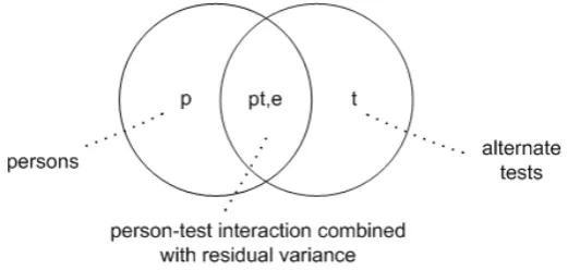
component. But in ordinary True Score Theory the error component derives from one single undifferentiated source of variance. In an alternative forms reliability study this source of error variance is the interaction between persons and tests, in a tes

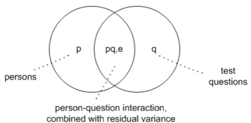
reliability study it is the interaction between persons and occasions (of testing), in a split half reliability study it is the interaction between persons and subtests, and in an internal consistency reliability study (KR-20 and alpha) it is the interaction between persons and test questions. These different possibilities for quantifying reliability lea to as many different reliability coefficients, each depending on the nature of the conceptualised measurement error – in G-theory terms we might say depending on assumptions made about the relevant ‘universe of generalisation’ (respectively, the universe of substitutable tests, the universe of testing occasions, the universe of h tests, or the universe of test questions).

In G-theory the error component can be broken down into several different subcomponents, the contributions to erro

‘generalizability coefficient’. This is one of G-theory’s principal strengths. I importantly, offers a “what if?” facility, which allows us to use information about contributions to measurement error to see how we might improve assessment procedures to reduce this error in future applications. This is its second principal strength.

Also in contrast with conventional True Score Theory, which addresses only one t of measur

the aim is to make mastery or grading decisions with maximum confidence when applying criterion cut scores to test results, such as in National Curriculum testing, school leaving qualifications and workplace assessment.

G-theory as originally formulated is underpinned by the conceptual and computation apparatus of the analysis of variance (ANOVA), which pr

al ovided the machinery eeded for extracting whatever variance components were called for by the

e eliability.

ity first appeared in the 1960s and ‘70s. In particular, the nalysis of variance, if viewed merely as a collection of procedures for manipulating

omplicated variance structures. It also makes accessible the extensive experience in

nd 4. r 3 we offer a reworking of the standard True Score Theory reliability dices, described earlier in this chapter, using unified G-theory tools and techniques.

ore n

investigator. The analysis of variance freed measurement theorists from having to work with only two variables at a time. With conventional reliability analyses, th experimenter must choose, for example, between test reliability and marker r Using analysis of variance techniques, item, person and marker effects could all be included in the same analysis, leaving it to the investigator to decide which of these contributed to the ‘true score’ variance and hence to determine the numerator of the reliability coefficient.

Statistical and computational theory and practice have moved on, of course, since the theory of generalizabil

a

relatively simple linear models and extracting their variance components, is now effectively subsumed into more sophisticated, encompassing constructs like

Generalized Linear Models (Dobson & Barnett, 2008; McCulloch, Searle & Neuhaus, 2008) and Multilevel Models (Snijders & Bosker, 1999; Goldstein, 2003).

As a conceptual tool, however, G-theory continues to offer valuable insights into the subtleties of determining reliability through the partitioning and unravelling of often c

experimentation and survey design that form an inseparable part of its ANOVA heritage.

The variance structure approach to reliability is discussed further in Chapters 3 a In Chapte

in

3 The variance components model

3.1 Reliability coefficients and standard errors of measurement

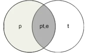
We have outlined in Chapter 2 the evolution in reliability conceptualisation from the correlational approach of the early pioneers to the variance analysis approach of G-theory. The consolidating role of G-theory in this evolution is very clear. G-theory has replaced the traditional reliability indicators of True Score Theory (alternate forms, test-retest, split half and also Cronbach’s α), by subsuming them as special cases in a more all-embracing conceptualisation. G-theory is a random sampling model, which, under the usual assumptions of linear modelling, provides a means of estimating the precision of measurements in situations where these measurements are subject to multiple sources of error (Cronbach, Gleser, Nanda & Rajaratnam, 1972; Cardinet & Tourneur, 1985; Shavelson & Webb, 1991, 2006; Brennan, 1992, 2000, 2001b; Cardinet, Johnson & Pini, 2009; Raykov & Marcoulides, 2010, Chapter 9). It is therefore an approach with natural potential for exploitation in the context of educational testing and examining, whether academic, vocational or professional. For each type of measurement there is an appropriate form of reliability, quantified in a G coefficient. The ‘coefficient of relative measurement’, Eρ2, was the coefficient

that Lee Cronbach originally defined as the generalizability coefficient. This

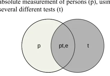
coefficient enables us to estimate how precisely an assessment procedure can locate individuals, whether pupils, examination candidates or company employees, relative to one another on a measurement scale. The ‘coefficient of absolute measurement’, Ф, that Brennan and Kane (1977a, 1977b; see also Brennan, 2001b, p.35) defined as the ‘dependability coefficient’, evaluates the ability of a procedure to locate individuals reliably on an absolute scale.

The formula for Ф is identical with that for ρ2, any difference in computed value being due to the fact that in absolute measurement there are typically more

contributors to error than there are in relative measurement. Developed at the same time as Ф by Brennan and Kane (1977a, 1977b), Ф(λ), a ‘coefficient of criterion-referenced measurement’, addresses cut score applications (Brennan, 2001b, p.48). This coefficient indicates how reliably an instrument can locate individuals with respect to a cut score, λ, on the measurement scale, with clear implications for the possibility of misclassification.

Each G coefficient is a ratio of true (or universe) score variance to the combination of true score variance and measurement error variance. Informally, we could consider this as a kind of signal-to-noise ratio, except that the denominator includes both signal and noise (signal-to-noise ratios also exist – see Brennan & Kane 1977b and Brennan 2003, pp.14-15). G coefficient values are in the range 0 to 1, as for α, with 1

indicating perfectly reliable measurement, 0 indicating totally unreliable

measurement, and 0.7-0.8 generally agreed as the range of lowest acceptable values for scores to be considered ‘reliable’. Criterion values are relatively arbitrary choices, and an ‘acceptable’ coefficient value could be different for different kinds of

The square root of the measurement error variance is the standard error of

measurement, or SEM, which is a measure of score precision (not accuracy, which has to do with how valid, as in ‘on target’, the measurement is). In G-theory the SEM relates to an average score, which in an examining context would typically be an examinee’s average test score (over several tests) or average question score (over the questions in a single test). As such it is based on the same metric as the average score that it refers to. In other words, if we have a test comprising questions each carrying three marks then the SEM for an individual’s average question score will also be estimated on a 0-3 scale. To produce an SEM for a total test score the average score SEM is simply multiplied by the number of questions that comprise the test. Under Normal distribution assumptions we can use the SEM to produce confidence intervals around the appropriate score estimate in the usual way.

The SEM is a critical piece of information to consider, and is at least as important as calculation of reliability coefficients. It was already being proposed as the most appropriate measure of score reliability 40 years ago, by Skurnick and Nuttall (1968), in the context of classical True Score Theory. Most recently, reflecting on his

lifetime’s work, Cronbach himself identified the facility to calculate the SEM as the essential contribution of G-theory (Cronbach and Shavelson, 2004). Use of the SEM is also recommended in the US Standards for educational and psychological testing (AERA/NCME/APA, 1999). In many modern-day applications, particularly in workplace assessment, where variance ratios are often meaningless by default, the SEM is the only useful indicator of reliability.

As noted by Raykov and Marcoulides (2010, Chapter 9), “the notion of a universe lies at the heart of generalizability theory”. In the G-theory approach, therefore, the first requirement is to identify the intended universe of generalisation. This means identifying all observable factors that can be assumed or suspected to affect the dependent variable, which in this context is an individual’s test score or other form of assessment outcome such as a rater judgement, to decide over which of the factors the assessment outcome is to be generalised, and to note which factors are being

implicitly or explicitly sampled in the assessment procedure. Those factors that are sampled will potentially contribute to measurement error. Test questions or

assessment tasks, along with markers, raters, workplace assessors or verifiers, are examples. So also are essay topics, item formats, and so on.

It is rarely the case that the particular questions used in a test are the only ones of interest for subject assessment. They are therefore by default a sample of all the questions that might have been used in their place, and they will in consequence contribute to measurement error. Similarly, the markers employed to evaluate test and examination performances are seldom of interest in their own right. They, too, are essentially sampled from some marker population, comprising actual or potential markers, and they too will contribute to measurement error. Ignoring the sampling status of questions, or modifying the characteristics of the marker samples, for

example through the usual procedure of standardisation, will typically result in higher apparent assessment reliability, but this will be at the cost of the validity of the