University of Southern Queensland
Faculty of Engineering and Surveying
Development of an
Electronically Controlled
Thruster
A dissertation submitted by
Douglas James Jesshope
In fulfilment of the requirements of
Course ENG4111 and 4112 Research
Project
Towards the degree of
Bachelor of Engineering (Mechanical) /
Bachelor of Science (Physics)
i | P a g e
Abstract
The aim of this project was to investigate the aerodynamic and structural effects of modifying a Carbon Fibre Toyota Supra TRD 3000 GT Wing to perform dynamic angle of attack updates. These angular updates have been based on an ideal aerodynamic phenomena required under different operating conditions. High speed cornering would see the wing produce maximum downforce, while heavy braking can be enhanced by using the wing blade to create maximum drag.
The realizable k – ε turbulence model was used in a two dimensional representation of the problem within ANSYS FLUENT. This analysis determined that for all speeds, maximum downforce was achieved at a -15° angle of attack. Maximum drag occurred on the wing when it was deployed at -60°, while minimum drag was achieved at 0°.
The magnitudes of the forces obtained from the FLUENT analysis were then compared to data released for the standard Toyota Supra wing. This comparison showed that the downforce was increased by 46.97% over the standard wing.
A near field strain analysis was performed in order to ensure that the carbon fibre wing was capable of withstanding the added forces. An existing wing was loaded with weights in a fibre composite laboratory, while strain gauges measured the amount of strain present in the surface fibres.
ii | P a g e
University of Southern Queensland
Faculty of Engineering and Surveying
ENG4111 & ENG4112 Research Project
Limitations of Use
The Council of the University of Southern Queensland, its Faculty of Engineering and Surveying, and the staff of the University of Southern Queensland, do not accept any responsibility for the truth, accuracy or completeness of material contained within or associated with this dissertation.
Persons using all or any part of this material do so at their own risk, and not at the risk of the Council of the University of Southern Queensland, its Faculty of Engineering and Surveying or the staff of the University of Southern Queensland.
This dissertation reports an educational exercise and has no purpose or validity beyond this exercise. The sole purpose of the course "Project and Dissertation" is to contribute to the overall education within the student’s chosen degree programme. This document, the associated hardware, software, drawings, and other material set out in the associated appendices should not be used for any other purpose: if they are so used, it is entirely at the risk of the user.
Professor Frank Bullen
Dean
iii | P a g e
Certification
I certify that the ideas, designs and experimental work, results, analyses and conclusions set out in this dissertation are entirely my own effort, except where otherwise indicated and acknowledged
I further certify that the work is original and has not been previously submitted for assessment in any other course or institution, except where specifically stated.
Douglas James Jesshope
Student Number: 0050086431
________________________________
Signature
________________________________
iv | P a g e
Acknowledgements
I would like to acknowledge the following for their invaluable support and guidance throughout the course of this project:
- Dr Jayantha Epaarachchi, for his supervision of the overall project objectives and for his expert advice pertaining to the strain analysis section of the project.
- Dr Andrew Wandel, for his insight into the theory behind Computational Fluid Dynamics and for his generous support in developing a functioning model.
- Dr Ruth Mossad, for her advice on the reliability of the different k - ε models and general support provided in passing.
v | P a g e
Contents
ABSTRACT ... I CERTIFICATION ... III ACKNOWLEDGEMENTS ... IV LIST OF FIGURES ... VII LIST OF TABLES ... X
1 INTRODUCTION ... 1
1.1BACKGROUND ... 1
1.2SCOPE AND OBJECTIVES OF PROJECT ... 1
1.3RISK ASSESSMENT ... 3
1.4CONSEQUENTIAL EFFECTS ... 4
1.4.1 Sustainability Issues ... 4
1.4.2 Ethical Issues ... 4
1.5RESOURCE REQUIREMENTS ... 5
2 LITERATURE REVIEW ... 6
2.1AERODYNAMICS OF ROAD VEHICLES ... 6
2.1.1 Drag ... 6
2.1.2 Lift ... 10
2.2EFFECTS OF REAR WINGS ON VEHICLE DYNAMICS ... 13
2.3ACTIVE AERODYNAMIC AIDS ... 16
2.4COMPUTATIONAL FLUID DYNAMICS ... 19
2.3.1 The k - ε Turbulence Model ... 21
2.3.1.1 The Standard k – ε Model ... 22
2.3.1.2 The Renormalisation Group k – ε Model... 24
2.3.1.3 The Realizable k – ε Model ... 25
2.3.2 The k - ω Turbulence Model ... 26
3 METHODOLOGY – 3D MODELLING ... 27
3.1PRELIMINARY WORK ... 27
3.2DEVELOPING THE WING GEOMETRY ... 28
3.3DEVELOPING THE VEHICLE GEOMETRY ... 30
vi | P a g e
4 METHODOLOGY – 2D FLUID DYNAMICS MODEL ... 39
4.1DEVELOPING THE MODEL GEOMETRY ... 39
4.2MESHING THE DOMAIN ... 43
4.3MODELLING THE FLOW ... 47
4.3.1 The FLUENT Launcher ... 47
4.3.2 Problem Setup - General ... 47
4.3.3 Problem Setup - Models ... 48
4.3.4 Problem Setup – Materials & Cell Zone Conditions ... 50
4.3.5 Problem Setup – Boundary Conditions... 50
4.3.6 Problem Setup – Reference Values ... 53
4.3.7 Solution Setup ... 54
5 METHODOLOGY - STRESS ANALYSIS OF WING BLADE ... 57
5.1MATERIAL SELECTION ... 57
5.2NEAR FIELD STRAIN MAPPING OF EXISTING WING BLADE ... 58
5.3FINITE ELEMENT ANALYSIS OF WING BLADE ... 63
6 RESULTS AND DISCUSSION ... 67
6.1COMPUTATIONAL FLUID DYNAMICS RESULTS ... 67
6.1.1 Maximum Downforce Angle ... 67
6.1.2 Maximum Drag Angle ... 73
6.1.3 Minimum Drag Angle ... 76
6.2DYNAMIC EFFECT OF CHANGES ... 79
6.3MATERIAL PERFORMANCE ... 82
6.3.1 Near Field Strain Analysis ... 82
6.3.2 Finite Element Analysis ... 83
7 CONCLUSION ... 86
7.2FURTHER WORK ... 87
8 REFERENCES ... 89
APPENDIX A – PROJECT SPECIFICATION ... 91
APPENDIX B – RAW FLUENT DATA ... 92
APPENDIX C – DEVELOPMENT OF FORCES PER VELOCITY ... 96
APPENDIX D – NEAR FIELD STRAIN RESULTS... 107
vii | P a g e
List of Figures
Figure 2.1 – Vehicle Frontal Area (Hucho 1987). . . 7
Figure 2.2 – Typical CD Values for Common Cross Sections (Benson 2010). . . 8
Figure 2.3 – Flow Separation Comparison for Common Cross Sections. . . 8
Figure 2.4 – The Evolution of Vehicle Aerodynamics (Hucho 1987). . . 9
Figure 2.5 – The Effect of a Spoiler on Turbulence (Damjanović et al 2010). . . 12
Figure 2.6 – The Effect of a Spoiler on Drag and Lift (Hucho 1987). . . 12
Figure 2.7 – The Standard Toyota Supra Rear Wing. . . . 13
Figure 2.8 – The 1955 Mercedes SLR at Le Mans. . . 16
Figure 2.9 – The Bugatti Veyron 16.4 and its Airbrake at 55°. . . . 17
Figure 2.10 – The Aeromotions S2 Wing with Centreplate. . . . 18
Figure 2.11 – Boundary Layer Development on a Flat Plate. . . . 25
Figure 3.1 – The Sketched Wing Profile. . . . 28
Figure 3.2 – The SolidWorks Sketches. . . . 29
Figure 3.3 – The Final Wing Model. . . 29
Figure 3.4 – The Initial JZA80 Supra Model. . . 30
Figure 3.5 – The Alias Wavefront OBJ Format. . . . 31
Figure 3.6 – Quadratic Edge Collapse Decimation. . . 33
Figure 3.7 – 19,999 Face Mesh in MeshLab. . . 33
Figure 3.8 – 19,999 Face Part in SolidWorks. . . 34
Figure 3.9 – The Rhinoceros T-Splines Model. . . 35
Figure 3.10 – The T-Splines Function. . . 35
Figure 3.11 – Non-Manifold Edges. . . . 36
viii | P a g e
Figure 3.13 – Gaps between Faces. . . 37
Figure 4.1 – Blueprints of the 1996-2002 Toyota Supra. . . 39
Figure 4.2 – The 2D SolidWorks Assembly Model. . . 40
Figure 4.3 – The 2D Flow Model Domain (L = 4514mm). . . . 41
Figure 4.4 – The Overlapping STEP Imports. . . 42
Figure 4.5– The Final Domain. . . . 43
Figure 4.6– The Vehicle Mesh. . . 46
Figure 4.7 – The Named Selections. . . . 46
Figure 4.8 – The Model Menu. . . 48
Figure 4.9 – Contours of Y+ in the Standard Wall Function Model. . . 49
Figure 4.10 – Defining the Inlet Conditions. . . 51
Figure 4.11 – Convergence of Scaled Residuals (818 iterations). . . 55
Figure 4.12 – Resultant Forces on Relevant Zones. . . 56
Figure 5.1 – Strain Gauge Locations – Upper Wing Surface. . . . 59
Figure 5.2 – Strain Gauge Locations – Lower Wing Surface. . . . 60
Figure 5.3 – Wire Structure for Gauge 3. . . 60
Figure 5.4 – The Strain Testing Assembly. . . . 61
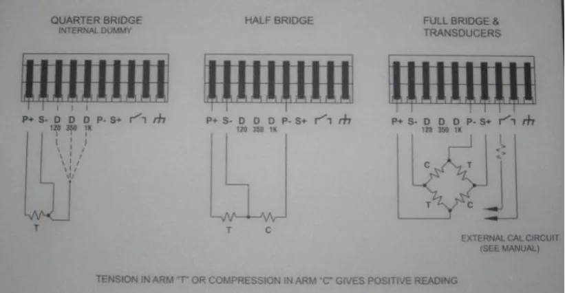
Figure 5.5 – The Half Bridge Connection. . . 62
Figure 5.6 – Isotropic verses Orthotropic. . . 63
Figure 5.7 – The Wing Mesh. . . 64
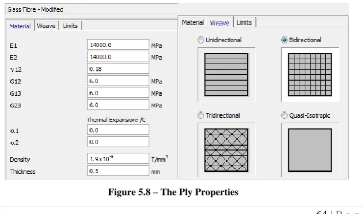
Figure 5.8 – The Ply Properties. . . . 64
Figure 5.9 – The Laminate Properties. . . 65
Figure 5.10 – The Load Case. . . 66
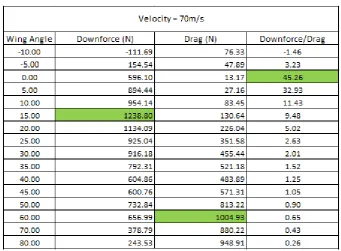
Figure 6.1 – Force versus Wing Angle (70 m/s). . . 68
ix | P a g e
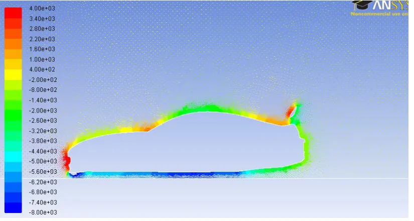
Figure 6.3 – Velocity Vectors Coloured By Static Pressure (Pascal). . . . 69
Figure 6.4 – Addition of Wheels to a car-like body (Hucho 1987 p165). . . 70
Figure 6.5 – Velocity Vectors Coloured By Velocity (m/s). . . 70
Figure 6.6 – Velocity Vectors Coloured By Velocity (m/s). . . 71
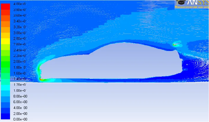
Figure 6.7 – Pathlines of Turbulent Intensity (%). . . 71
Figure 6.8 – The Maximum Downforce Wing Angle Forces (-15°). . . 72
Figure 6.9 – Velocity Vectors Coloured By Static Pressure (Pascal). . . . 73
Figure 6.10 – Velocity Vectors Coloured By Static Pressure (Pascal). . . 74
Figure 6.11 – Velocity Vectors Coloured By Velocity (m/s). . . 74
Figure 6.12 – Pathlines of Turbulent Intensity (%). . . . 75
Figure 6.13 – The Maximum Drag Wing Angle Forces (-60°). . . 75
Figure 6.14 – Velocity Vectors Coloured By Velocity (m/s). . . 76
Figure 6.15 – The Maximum Drag Wing Angle Forces (0°). . . 77
Figure 6.16 – Pathlines of Turbulent Intensity (%). . . . 77
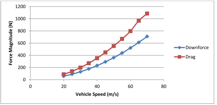
Figure 6.17 – Comparison of Vehicle Drag Forces. . . 78
Figure 6.18 – Strand7 Strain Plot (55 lb. Load). . . . 83
Figure 6.19 – Strand7 Strain Plot (1337 N Load). . . 84
x | P a g e
List of Tables
Table 1.1 – Details of Risk Assessment. . . 3
Table 3.1 – JZA80 Toyota Supra Specifications. . . . 27
Table 3.2 – TRD 3000GT Wing Dimensions. . . . 27
Table 4.1 – Span Angle Centre. . . 45
Table 4.2 – The Mesh Settings. . . 46
Table 4.3 – Reference Values. . . . 53
Table 4.4 – Solution Methods. . . . 54
Table 4.5 – Residual Monitors. . . 55
Table 5.1 – Selected Strain Gauges. . . . 58
Table 6.1 – Wing Angle Data at 70 m/s. . . 68
Table 6.2 – Minimum Corner Radius Decrease (40.3 m/s). . . 81
Table 6.3 – Minimum Corner Radius Decrease (70 m/s). . . 81
Table 6.4 – Strain Measured Within Wing Blade (55 lb.). . . 82
Table 6.5 – Strain Comparison of Wing Blades (55 lb.). . . 84
1 | P a g e
1 Introduction
1.1 Background
The Toyota Supra JZA80 is an iconic Japanese sports car and was produced from 1993 to 2002 in a range of trim levels. One of these trim levels included an addition of an active aerodynamic front lip spoiler that deploys at speeds in excess of 80km/h in order to improve the flow profile over the car. This project is aimed at complimenting the effects of this spoiler with the addition of an active rear wing that can be manipulated to enhance the performance of the car.
The project objectives, shown below in Section 1.2, outline the critical deflection angles for an active spoiler such as this. Obtaining wing angles that correlate to maximum and minimum drag forces over a range of vehicle velocities is paramount to the success of this project. In theory, a wing deployed at an angle that maximises drag will allow the car to brake more quickly than an identical vehicle with a standard wing angle. In a similar scenario, a wing deployed at an angle that produces minimum drag will allow the car to travel at a higher top speed than a car without that ability.
This project will explore both scenarios and determine if the magnitude of the calculated gains justifies the application of an active rear spoiler on a Toyota Supra. Furthermore, the methodology of this project will also examine the ability of the wing to increase the vehicles rear wheel tractive forces by providing downforce.
1.2 Scope and Objectives of Project
2 | P a g e
encompasses the mathematical, experimental and computational analysis stages of the dissertation.
The following should be considered for the product scope:
- The wing shall actuate to achieve maximum total drag force
- The wing shall actuate to achieve minimum total drag force
- The wing shall actuate to achieve maximum down force
- The wing actuation must not impair driver’s field of vision
- The final product must be designed to withstand increased stresses
- The wing exterior profile shall be unchanged from the TRD 3000GT Model
With the preceding comments in mind, the objectives for the product aspect of the dissertation will be to:
- Create a dimensionally accurate 2D CAD profile of the supra body
- Append a 2D CAD profile of the TRD wing at a large range of attack angles
- Perform 2D aerodynamic simulations on the model to obtain proof of concept
- Develop an accurate 3D CAD TRD wing model
- Perform FEA on the 3D wing to in order determine actuation stresses.
- Experimentally calibrate/confirm model accuracy using strain gauges.
Coinciding with the product objectives are the project objectives. These are outlined below and serve to improve the accuracy of the product objective results by exploring the successes and errors of similarly scoped projects. These objectives are:
- Research general automotive aerodynamics, including current airbrake designs
- Research 2D & 3D Fluent modelling platforms and select a suitable analysis
- Research the materials commonly used in relevant aerodynamic applications
3 | P a g e
1.3 Risk Assessment
As with any engineering project, there are risks involved with the execution of the project and product objectives. The observed and foreseen risks have been tabulated below in order to rank their severity and offer methods of controlling, eliminating or minimising the risks.
Description of Hazard Persons at Risk Risk Severity Exposure to
Risk Consequences
Control Measures Taken
Eyesight damage, due to long hours spent sitting at computer desk
Myself Slight Frequently Minor Injury
Avoid staring at the screen, Adjust brightness
accordingly, Take 5 minute break every 60
minutes.
Injury sustained from incorrect re-assembly of external vehicle body components.
Public Very
Slight Rarely
Major Injury/Possible
Death
Avoid working when overtired; Never work on
the car alone. Double-check components are
secure
Repetitive Strain injury to fingers
from typing
Myself Substantial Frequently Minor Injury
Ensure fingers are warm and adequately stretched;
Take 5 minute break every 60 minutes.
Damage to HDD and other PC Components from
continuous load
Personal
Computer Significant Continuously
Major Component
Damage
Simulate processes according to ANSYS specified requirements. Regularly back-up work
Blunt force injury resulting from weights dropping from testing stands
Myself, others in laboratory
Significant Rarely
Bruising, broken skin, broken bones
Follow WH&S Protocol in P2 Laboratory, wear
safety boots, maintain clearance about weights
Inhaling of toxic fumes whilst
soldering
Myself Significant Rarely
Damage to blood-forming, nervous & reproductive systems
Follow WH&S Protocol, wear a breathing mask when appropriate, ensure
fumes can escape local proximity.
Super glued digits whilst applying
strain gauges
Myself Minor
Injury Rarely Skin Damage
Ensure plastic aids are used to apply pressure to glued components when
necessary.
4 | P a g e
1.4 Consequential Effects
1.4.1 Sustainability Issues
The product deliverable will ultimately be designed to leech electrical power from the vehicles electrical energy reserves. As such, the sustainability of running such an item shall we weighted against the amount of electrical power it consumes. Design of the electronic components should be based about electrical efficiency in order to prevent a permanent drain that exceeds the alternators regeneration capacity.
Also, the addition of aftermarket wiring into a genuine production car loom could produce problems with genuine features within range of the proposed system integration. Items such as tail lights and reverse lights should be tested post installation to ensure functionality until a fool proof wiring integration diagram is formulated.
1.4.2 Ethical Issues
The original TRD 3000GT wing for the Toyota Supra is a copyrighted item and it is therefore prohibited to manufacture and distribute replica wings under the TRD company banner, or imply that the product is associated with the company in any way. It must be clearly detailed at all stages from the initial design phase, through to the completion of a prototype wing, that the active rear wing is an aftermarket replica.
Before constructing a wing for public demonstration or sale it is necessary to properly investigate the extent of the copyright associated with a genuine TRD wing. In the event that distinctive features such as the aerofoil geometries used for the original design are covered by patents or copyright, legal counsel should be sought.
5 | P a g e
1.5 Resource Requirements
The product and project scope objectives are heavily computer based and the resource requirements reflect this. For the project aspect of the report, a substantial amount of literature that describe the modelling, fluid dynamic analysis and finite element analysis must be discovered, interpreted and appreciated. On top of the discoverable literature resources will be the task specific knowledge that my supervisors use to guide my progress throughout the task.
The product based resource requirements are more clearly defined. In order to model the car in the required 3D manner, access to the following software packages in essential.
- Autodesk 3DStudio - MeshLab
- Autodesk Rhinoceros - SolidWorks 2012 - ANSYS
- Strand7
Most of these are very memory intense applications and as such a computer capable of running these is also required. The project objectives utilized an Intel i7 processor and 8GB RAM which proved sufficient. The product objectives were limited to running on significantly slower dual core computers, which greatly impacted upon processing time.
Fluid dynamic software was required to run iterations of the model over several geometry changes. This required another ANSYS product called Fluent. The university computers were sufficient to model the 2D flow in a timely fashion. It is indicated in the reviewed literature that 3D analysis of fluid flow over a meshed car body is an extremely detailed process that exceeds the abilities of these computers.
6 | P a g e
2 Literature Review
A literature review was performed in order to gain a solid understanding of the theoretical, computational and practical aspects of designing an aerodynamic based vehicle component. The sources included fluid mechanics textbooks, journal articles, driver’s accounts, manufacturer’s specifications and fluid mechanics reference material.
2.1 Aerodynamics of Road Vehicles
Road vehicles are subject to a large range of aerodynamic effects that can greatly alter the performance and stability of the vehicular motion. Aerodynamic drag, side wind stability and tail lift are unbalanced pressure forces that act upon the shell of the vehicle and alter the dynamics of motion.
2.1.1 Drag
Of the forces listed above, aerodynamic drag is the more prominent hindrance to motion. Drag is the force that acts directly opposite to the direction of motion and is caused by a combination of friction and viscous components. The viscous component is the result of turbulence created by the vehicle body and is the most significant component when considering vehicular motion. Hucho (1987, p2) states that at a speed of 100km/h, the aerodynamic drag resisting the forward motion of a mid-sized European car of that time was in order of 80% of the vehicles total road resistance.
7 | P a g e
( )
( )
( ) ( )
( )
This shows that the drag force that acts on the vehicle is proportional to the frontal area (A), the pressure of the air (ρ), the vehicle velocity (V) and a vehicle shape factor ( ) called the drag coefficient. As such, the critical factors for decreasing the overall drag of a vehicle are the frontal area and drag coefficient.
The frontal area is measured as the total two-dimensional area “seen” by a viewer from the front of the car. Car designers are quite restricted when it comes to reducing this area as the ergonomics of the driver and passenger seating positions define a large percentage of the total frontal shape. This restriction is shown below.
Therefore the most effective factor available to manipulate in Equation 2.1 is the vehicles drag coefficient. The drag co-efficient is a dimensionless factor that describes the magnitude of aerodynamic hindrance a bluff body has on the flow passing over it. The smaller the coefficient, the less air resistance that object will incur when traversing through the air.
8 | P a g e
Bluff objects with rapid geometry changes perpendicular to the flow direction, such as cubes, prisms and spheres, tend to have a high drag coefficient. Conversely, bluff objects such as aerofoils that have very small changes perpendicular to the flow direction have very small drag coefficients.
Rapid changes in bluff object geometry result in separation of the flow field and the object surface. When a flow passes over a body, it attaches itself to the external contour of that shape and attempts to follow along the surface until its end. Rapid geometry changes prevent this by creating vacant zones, such as the on right hand side of the circular section below.
This flow separation effect is the one of the main contributors to aerodynamic drag on motor vehicles. When the flow separates from the surface of the vehicle, pockets of air with near-atmospheric properties fill the void left between the surface and the streamlines. This air is generally turbulent and dramatically increases the drag force acting upon the vehicle.
Early motor vehicles were not designed with aerodynamics in mind and as a result they had very tall, largely angular passenger compartments. As aeronautic
Figure 2.2 – Typical CD Values for Common Cross Sections (Benson 2010)
9 | P a g e
technology advanced, the results slowly made their way across into the motor vehicle industry.
As vehicles became faster, the aerodynamic effects on the body became more significant. As such, the tall, orthogonal body styles from the early 1920’s were replaced with lowered and more streamlined designs by 1940 after the mainstream application of aerodynamic principles. Vertical windscreens were replaced with inclined examples that allowed the air flow to remain attached to the vehicle shell, resulting in significantly smaller drag coefficients.
The end of World War II brought about a new era in the development of aerodynamic shapes for vehicle design. Race engineers began experimenting with wind tunnels in order to evaluate the aerodynamic capabilities of their vehicles and aerodynamic components. These changes would eventually make their way into designs for production cars. The evolution of productions cars continues to gain inspiration from competitive motorsport.
In recent years, the experimental testing of new concepts has been predominantly computer based now that the technology is available, however wind tunnels are still used for validation of computational results. These improvements have allowed the drag co-efficient of production vehicles to reach between 0.2 and 0.3, an incredible decrease when comparing to the corresponding vehicles made in the 1980’s.
10 | P a g e
2.1.2 Lift
Lift is the force that acts perpendicular to the direction of vehicular motion. The lift force is similar to drag in that it is calculated from the velocity of motion and properties of the displaced fluid. In all cases, lift is measured upward with respect to the body according to the equation below.
( )
( )
( ) ( )
( )
This phenomenon has a far smaller effect on production vehicles than drag as it has a very small magnitude at speeds below 100 km/h. Also, the lift force does not inhibit the motion of the vehicle. For this reason, most production vehicles do not employ aerodynamic aids that are specifically designed to develop a negative lift force. Most modern, road based vehicles use aerodynamic aids that decrease the lift co-efficient of the vehicle, while also decreasing the drag acting against the vehicle.
The name given to this common aerodynamic aid is a ‘Spoiler’. The addition of a spoiler essentially disrupts the flow over the rear end of the vehicle. The main effect of this is to spoil the high velocity nature of the airstream without increasing drag. This reduces the magnitude of the lift force created by the high velocity, low static pressure air according to Daniel Bernoulli’s equations for fluid in a streamline.
( )
( ) ( ) ( ) ( ) ( )
11 | P a g e
elevation pressure. In that case of a moving vehicle or aerofoil, it can be assumed that the elevation pressure is constant at all points along the streamline given that the elevation change will be negligible. This results in Equation 2.3.1
( )
As such, when the velocity of a fluid flow increases, the static pressure that can be measured within that flow is decreased to satisfy the equation. Consider the case when a vehicle is travelling through a body of air at a constant total pressure.
The body of the air travelling along the upper side of the vehicle has significantly further to travel than the air travelling under the body. As the air on both sides of the vehicle had the same properties prior to being separated, they both have the same constant total pressure. The air that travels the furthest will be forced to accelerate to a higher velocity by the air particles that are behind it on the streamline. This faster moving air will now have a smaller static pressure value, as some of the pressure has been changed to dynamic pressure during the velocity increase. Therefore, there is a discrepancy between the static pressures of the air on the upper and lower side of the vehicle. A lift force results from this imbalance, as the high static pressure side pushes the vehicle upward, while the low static pressure side pulls the vehicle in the same upward direction.
Another effect of a spoiler is to prevent the flow from forming a large stagnant air pocket that would normally be created when the flow moves to fill the void left by the body. The act of diverting the airflow effectively increases the overall length of the vehicle and allows for a more steady integration of the vehicle airflow back into the free stream, greatly reducing drag.
12 | P a g e
The application of spoilers will have varying effects when different vehicles are considered, however the general consensus is that a correctly designed spoiler can have a dramatic effect on the drag and lift coefficients of a standard motor vehicle. Hucho (1987) showed this in his wind tunnel experiments on a Volkswagen 1600 coupe. He performed comparative testing on a number of simple aerodynamic attachments in order to gauge the effect that each had on the lift and drag forces. The results of this comparative testing to the overall lift and drag coefficients of the Volkswagen 1600 are shown below.
The lift coefficient of the vehicle was more than halved by the addition of the spoiler, while the drag coefficient also went down marginally due to the effect shown in Figure 2.5. Further research done by Wolf-Heinrich Hucho has shown that this overall vehicle lift co-efficient can be broken down and separated into wheel-axle specific coefficients in order to gauge the effect that lift forces have upon the front and rear reaction forces acting through the vehicles tyres.
Figure 2.5 – The Effect of a Spoiler on Turbulence (Damjanović et al 2010)
13 | P a g e
2.2 Effects of Rear Wings on Vehicle Dynamics
Another common aerodynamic aid used on production vehicles is the rear wing. Often confused for a spoiler, a rear wing is actually an inverted aerofoil that is located further from the vehicle surface than a spoiler. This allows the aerofoil to interact with incoming air that has a more developed, consistent velocity.
The inverted aerofoil actually produces a localised negative lift force that pushes the rear of the car back down toward the road surface, negating the effects of the rear end lift discussed earlier. However, as a result of being employed higher within the flow, the aerofoil actually increases drag forces in many cases.
An example of this rear wing attachment is the standard wing for the Toyota Supra. The cross section of this wing is a non-symmetrical inverted aerofoil with a significantly smaller vertical depth than the Toyota Racing Development replacement used in this analysis. Toyota released the aerodynamic figures relating to this wing shortly after the vehicle’s release in 1993. According to their development data, the aerofoil added 66 lb. of negative lift force while the vehicle was progressing at 90 mph.
This equates to approximately 294 Newtons of downward force on the car at 145 km/h and acts directly against the rear end lift forces, pushing the rear tyres into the road surface. On Australian roads, this is much faster than the vehicle should be travelling, which means that the wing only produces a small proportion of the total
14 | P a g e
apparent vehicle mass at legal speeds. As such, the wing may provide extra stability during highway driving but it will not markedly increase the performance characteristics of the vehicle.
The addition of the rear wing to the Toyota Supra also increases the drag co-efficient of the vehicle from 0.31 to 0.33. This means that the incurred drag will increase by approximately 6.5% at all speeds, which is a significant increase when the car is not used off-road. However, if the car is used off road, the effects of the rear wing can greatly increase the downward forces at the rear of the vehicle. This is where the application of a rear wing can truly be justified.
Isaac Newton showed that a centre force acts upon a body in circular motion according to the following equation:
( )
( ) ( ) ( ) ( )
It is also known that a vehicle in motion can only use the frictional force to negate the outward push of the centre force. This friction force is the proportional to the coefficient of friction between the tyres and the road, while the normal force is the amount of upward reaction force pushing against the tyre.
That is:
( )
( ) ( )
15 | P a g e
Equation 2.6 shows that for a vehicle turning a corner with a constant radius, velocity is directly proportional to the amount of normal force being applied to the vehicles tyres. At sufficient speeds, i.e. above 115 km/h, the downforce produced by the rear wing on a vehicle increases the normal force being applied to the tyres. This in turn increases the maximum speed at which the vehicle can travel around that corner.
This mathematical relationship is the basis for front and rear wing geometries being added to many classes of racing. The most elite of these racing classes is Formula 1, which allows its vehicles to employ numerous wing attachments. According to the Official F1 website (2012), modern Formula 1 vehicles are ‘capable of developing 3.5 g lateral cornering force thanks to aerodynamic downforce’.
However, this acceptance of increased grip through the use of aerodynamics has not been without critics. Sorensen et al (1999) showed the dramatic effect that increasing traction through the use of aerodynamics puts the drivers at risk of serious injury. Equation 11 of their paper states:
( )
Through mathematical reasoning, they proceed to show that when a vehicle is travelling through a corner using increased tractive ability and vehicle control is lost, it spins and all of the aerodynamically added normal forces disappear. This results in the available friction force described in Equation 2.5 will decrease in the same proportions, assuming that the vehicle remains on the same type of ground. The work done by the friction force after control is lost is shown below:
( )
16 | P a g e
2.3 Active Aerodynamic Aids
The traditional approach to vehicle aerodynamics is to create a compromise between optimum performances in a certain number of scenarios. According to a release by Daimler-Chrysler (2012), the first person to implement an active aerodynamic aid on a vehicle was Alfred Neubauer when he developed the idea of an ‘airbrake’ in 1955. This concept was dreamt up by Neubauer, is his capacity at Mercedes’ Director of Motorsport, when he proposed it as a solution to overcome the excessive wear that occurred on the drum brakes of Mercedes 300 SLR Le Mans car.
This brake is shown in Figure 2.8 and has an area of 0.7 m2. A hydraulic pump was used to deploy the brake when the car experienced heavy braking. The result was significant, with the brake increasing both the braking and cornering abilities of the vehicle.
Some of the first production vehicles to utilise active aerodynamic aids were the Volkswagen Corrado and the Lancia Thema from 1986. Rather than implementing a large braking aid like the Mercedes, these vehicles were designed with active rear spoilers. These spoilers are deployed electronically and act to reduce the drag acting on the vehicle when travelling at high speeds. This innovation was specifically aimed at improving the efficiency of the vehicles, rather than their sports based performances.
17 | P a g e
Several performance vehicles adopted active aerodynamic technology during the 1990’s. Cars such as the Mitsubishi GTO VR4 (1991-1996), the Toyota Supra JZA80 (1995-2002) and the Nissan Skyline R32/R33 (1990-1998) all used active front spoilers that lowered below the front bumper in order to restrict the amount of air that could flow beneath the vehicle. This acted to reduce the amount of lift that was produced by high pressure systems beneath the vehicle.
The most infamous road vehicle to utilise an active aerodynamic aid is the Bugatti Veyron 16.4, released in 2005. It gained this status by becoming the first production vehicle to utilize and active aerodynamic aid that also acted as an airbrake. According to the manufacturers website, when the Veyron is braking from very high speeds (above 200 km/h) the twin blade airbrake deploys at an angle of attack of 55°. This is shown below in Figure 2.9.
This action allows the Veyron to increase its rate of deceleration by 0.6 times Earth’s gravitational pull, or 5.89 m/ss. To put this in perspective, that rate of deceleration is equivalent to the maximum deceleration felt by recently released small vehicle. While this addition may not prove particularly useful on a public roadway, it is an invaluable asset when used on a racetrack.
The design of this airbrake would prove difficult to reproduce when modifying a regular production vehicle. The complex hydraulic system that actuates the wing blade angles have been recessed into the rear hatch of the Bugatti, as shown in Figure
18 | P a g e
2.9. It would take a large amount of customised bodywork and manipulation of standard systems in order to retrofit the Supra with a design similar to this.
One company that recognised this fact was Aeromotions. A group of engineers from the Massachusetts Institute of Technology (MIT) developed an aftermarket dynamic rear wing for a Nissan R35 GTR through full vehicle computational fluid dynamics analysis. This allowed the company to use the MIT wind tunnel to develop an optimum blade design for high downforce and low drag forces.
The wing shown below is the Aeromotions S2 dynamic rear wing. It is constructed of high shear modulus carbon fibre and utilizes a centre plate to ensure that cross transfer of the flow cannot occur. Both the uprights and the mounting points have been moulded into teardrop shapes to minimise the drag that these features induce.
The basic twin-turret design allows this model of wing to be retrofitted to many different vehicles with ease, while the high strength materials have allowed this wing to be approved for use in on public roads in several countries. The data speaks for itself, showing that this wing takes an average 2.29 seconds per lap off for a large range of vehicles on a track with an approximate two minute lap time.
The active version of the TRD wing should be based closely upon the geometry setup of this wing. The actuators should be hydraulic pistons that are located within the standard aerofoil shaped side turrets. Control boxes could then be located on the underside of the hatch, where wiring is already present.
19 | P a g e
2.4 Computational Fluid Dynamics
According to Bakker (2006) there are three equation forms that form the basis of computational fluid dynamics. The equations were derived from Euler’s equations for the conservation of mass and momentum. These Navier-Stokes equations expand upon Euler’s equations by allowing for the introduction of the fluid viscosity. The final equation used is the first law of thermodynamics that describes the conservation of energy.
The steady state equation for the conservation of mass states that the sum mass flux across Cartesian component boundaries within a control volume will be zero.
That is:
( )
The momentum equations apply newtons second law of motion to each of the three dimensions and show that a change in particle momentum in a component direction will be balanced by equal and opposing changes to momentum in other directions. The equations shown below describe the conservation of momentum within a steady state reference frame.
That is:
( )
( )
20 | P a g e
The conservation of energy equation demonstrates that energy can neither be created nor destroyed. It is merely transferred into a different form, ranging from kinetic, potential, light or heat to name a few. The Navier-Stokes representation of this principle that is specific to energy within fluid flow is shown below.
That is:
( )
Computational fluid dynamics programs can utilise all three of these Navier-Stokes equations in order to analyse the flow of a non-turbulent Newtonian fluid within a control volume. A fluid is classified as Newtonian if its properties satisfy the following equation.
( )
( )
( )
( ) ( )
21 | P a g e
2.3.1 The k - ε Turbulence Model
The k - ε turbulent model allows for the introduction two new equations that describe the turbulent nature of the flow. These equations, in parallel with the governing equations above, provide the fluid mechanics software with sufficient information to calculate an accurate flow field.
According to Scott-Pomerantz (2004) the first k - ε model was by developed by Harlow and Nakayama in 1968 at the Los Alamos Science Laboratory. These equations describe the dynamic nature of turbulent flow, which led to them inheriting the functional description of ‘transport equations’. These equations are shown below.
( ) ( )
( ) ( )
According to Savli (2012) turbulent kinetic energy describes the energy contribution that turbulent eddies within a mean flow have to the overall kinetic energy of that flow. The mean kinetic energy of a flow can be calculated by taking the kinetic energy of the flow using the mean flow speed in the following equation.
( ̅ ̅ ̅ ) ( )
22 | P a g e
Turbulent kinetic energy expands on this mean energy by taking the root mean square (RMS) of velocity fluctuations within the flow field. This value encompasses all the normal stresses contained within the flow and is described by the equation below.
( ̅ ̅ ̅̅̅ ) ( )
This allows for the calculation of the turbulent intensity contained within a flow. The second equation for turbulent dissipation rate mathematically describes the natural law that turbulent eddies will decrease in intensity and energy as time passes.
As the turbulent kinetic energy contained within a flow is subject to change, the main focus of computational fluid mechanics is on the turbulent kinetic energy budget. This budget describes the rate of change of the turbulent kinetic energy over time.
2.3.1.1 The Standard k – ε Model
(Launder et al. 1972) recognised this when they derived the true numerical transport equations for computational analysis of turbulent flows. These equations have become the basis of modern day two-equation turbulence modelling due to their economical delivery of accurate results when applied correctly. According to the ANSYS Help file, the mathematical derivation of the following equations assumes that the analysed flow is fully turbulent and that the molecular viscosity is negligible. As such, all k – ε models are only valid for turbulent flows. The equations that describe the standard form are shown below.
( ) ( ) [( )
] ( )
( ) ( ) [( )
23 | P a g e
( )
( )
For the analysis of subsonic flow, the compressibility term can be ignored as the fluid used within this analysis is incompressible under the scenario conditions. These equations are used by the software in order to calculate the turbulent viscosity of the fluid body. The equation for this calculation is as follows.
( )
(Damjanovic et al. 2010) used this standard form of the k – ε model with the following default values in their 2D analysis of airflow about a conceptual vehicle.
24 | P a g e
This allowed the group to model the effects of turbulence to a sufficient degree of accuracy without exploring the effects of changing the model to a more suitable, near wall specific model. However, it this group had researched further, they would have been able to recognise that this standard k – ε model was specific to high Reynolds number flow. As their flow was at relatively low speeds in the subsonic range, a more specific model would have increased the accuracy of the results.
2.3.1.2 The Renormalisation Group k – ε Model
Since their inception in 1972, the k – ε have been modified into a number of different forms that optimise the numerical equations for uses in specific applications. One of the newer k – ε models is called the renormalisation group model which was formulated in Yakhut and Orzsag (1986). This model improves on the low Reynolds number computation of the standard k – ε model. It introduces a new term into both of the base transport equations in order to allow the software to more accurately model rapidly strained flow. These types of flows include turbulent swirls and vortices that often occur in the near wall region when geometries change rapidly. Provided that the near wall treatment values are set up correctly, this solution is significantly more adept at modelling near wall flow. Interestingly, the change in Reynolds number focus only reduced the Cµ to 0.0845, still close to the standard.
(Roumeas, Gillieron & Kourta 2008) utilized this enhanced accuracy in their three dimensional reconstruction of a previously 2D flow analysis. Their investigation was based about the effect that an applied suction has on the flow separation over the rear of a Renault hatchback. As their analysis was specifically focussed on the near wall effects of separation vortices on the drag produced behind the car, this model was the ideal choice.
25 | P a g e
2.3.1.3 The Realizable k – ε Model
The last commonly applied k – ε model is called the realizable model. This model improves on the previous two equations by allowing the Cµ term to be varied based upon the properties of the fluid within the turbulent boundary layer development. This turbulent boundary layer is where the velocity gradient of the flow develops the most rapidly. As such, accurate modelling of the fluid properties in this region is vital to the accuracy of the solution.
The realizable model sets the Cµ term to approximately 0.09 within a logarithmic development layer of the fluid boundary layer, in keeping with values of the first two models discussed. However, when flow is deemed to be flowing with a strong homogenous shear the value for Cµ can drop as low as 0.05, far below that of the previous models.
The realizable model gains its name from (Shih et al. 1995) because it has added mathematical features that ensure the physics of the flow conform to the theory of turbulent flows in regards to Reynolds stresses. Shih also modified the turbulent dissipation transport model away from the approximate value used to the first to models. Shih’s realizable model uses a mathematically exact formula instead, which was derived from an existing vorticity fluctuation formula. For this reason, the realizable model is considered mathematically advanced. According to the ANSYS
26 | P a g e
Help file, one of the only negative aspects of the realizable transport model is its inability to accurately model multiple reference frames due to the changes to the transport equations.
(Mafi 2007) shows how adept the realisable k – ε model is at simulating low Reynolds number turbulent flow in his investigation into turbulence reduction at the rear of a Formula 1 vehicle. Mafi uses a very fine mesh within a 2D domain in order to determine the negative lift performance of a rear wing that diverts a significant portion of the airstream upwards when deployed at large angles. After the general case is solved he again uses the realizable model, this time in 3D form, to analyse the vortices present in the upward flow.
2.3.2 The k - ω Turbulence Model
The other form of two equation fluid modelling within ANSYS is called the k – ω turbulence model. This model still uses an equation for the turbulent kinetic energy within the flow, but it replaces the turbulent diffusivity equation with a term called the specific dissipation rate. Its base equations are shown below.
( ) ( ) [
] ( )
( ) ( ) [
] ( )
27 | P a g e
3 Methodology – 3D Modelling
This section of the document details steps taken in the modelling process, ranging from the wing geometry to the mesh and surface modelling of the vehicle body.
3.1 Preliminary Work
Before any work could begin on setting up the problem, the parameters required in order to construct, model and evaluate the analysis needed to be discovered and compiled. This section acts as a reference guide for all the following steps.
The leading edge at the centre of the wing is 20 mm closer to the rear of the vehicle and raised 10 mm above the corresponding point on each side.
Toyota Supra Specifications
Length 4514 mm
Width 1810 mm
Height 1245 mm*
Track (front/rear) 1520 mm / 1525 mm
Wheelbase 2550 mm
Ground Clearance 100 mm*
Mass 1550 kg (53%F/47%R)
Drag Co-efficient 0.33 (with wing)
Top Speed 250 km/h (restricted)
* Modified height in compliance with minimum legal Ground Clearance
TRD 3000GT Wing Dimensions
Width 1080 mm
Chord Length 230 mm
Table 3.1 – JZA80 Toyota Supra Specifications
28 | P a g e
3.2 Developing the Wing Geometry
The process of developing a computer based model of the TRD 3000GT wing began with the dismantling and measurement of an existing carbon fibre wing blade. Using some thin cardboard sheet, scissors and a thin tipped permanent marker, the upper and lower contours were traced. This was achieved by requesting that a partner align the cardboard sheet perpendicular to each contour at the centreline of the wing. The thin tipped marker was then guided across the wing surface, tracing the contour onto the cardboard sheet. The sheet was then removed and scissors were used to cut along the traced line. This process was repeated several times, bringing the shape of the remaining card closer to the actual wing shape each time.
Once the upper and lower contours had been successfully reproduced, they were both fixed in place over a sheet of A4 paper. This allowed both contours to be traced onto a single sheet. The resulting sketch was then scanned to JPEG format, resulting in the image shown below.
This image could then be imported into AutoCAD 2012 as a raster image reference. After this, the closed loop spline curved tool was used in order to draft over the sketched lines. The resulting curve was then measured electronically to ensure that its scale and overall dimensions accurately reflected the true dimensions of the existing wing.
The AutoCAD sketch satisfied the dimensional checks and was then imported into SolidWorks to act as the basis for the 3D model. Further measurement of the wing showed that the overall length was 1080mm from face to face, with these faces
29 | P a g e
parallel to the centreline. The cross section differed minimally across the span of the aerofoil and as a result it was concluded that a constant cross section model was suitable. The leading edge at the centreline of the wing was 20mm closer to the rear of the vehicle and raised 10mm above the corresponding point on each face.
From this data, another spline curve was drawn in SolidWorks that represented the location of the leading edge at all distances across the span of the wing. This curve intersected the leading edge of the imported aerofoil profile, allowing a spline extrusion of that profile across the span. A further addition to the extrusion process was the second, smaller aerofoil profile that was created using an offset distance of 2mm.
Once these profile sketches were finalised, both were extruded along the guide curve in order to form a 2mm thick solid body, where the larger profile was the outer shell and the smaller profile described the inner. The 2mm thickness was selected from Vernier calliper measurements of the carbon fibre weave of the existing wing. The end faces of the extrusion were then trimmed back to square as per the existing wing, with 2mm thick end caps added to form the final product, shown below.
Figure 3.2 – The SolidWorks Sketches
30 | P a g e
3.3 Developing the Vehicle Geometry
The vehicle geometry is considerably more complex than the wing and it was clear that a comprehensive tutorial or dimensional guide would be needed in order to prepare an accurate model. However, a lengthy search of solid modelling tutorial sites proved fruitless. As such, it was decided that pre-existing scale models could be used in place of creating a new file. A suitably well-constructed model was obtained free of charge from a computer model sharing site. This model had been constructed in Autodesk’s computer modelling package, “3DS Max”.
This program allows software companies to create 3D graphic animation models for video games and cartoon films. Unlike engineering based modelling suites, this application focusses more on the graphic appeal than rigid relationships between neighbouring features. This allows the user to freely use push and pull functions to quickly construct complex shapes from base objects.
Despite this relative lack of accuracy when compared to equivalent engineering programs, the overall dimensions of the vehicle, shown above, were in exact proportion to the actual vehicle. A trial version of the 3DS Max program was downloaded and the model was stripped of all non-essential features in order to decrease the size of the file and minimise the processing power required to manipulate the shell. These features included the interior, wheels, brakes, standard rear wing, antenna, door handles, windscreen wipers etc.
31 | P a g e
The next step in the process was to save the cleaned up geometry as a file type that could be supported by SolidWorks 2012, as the native 3ds format was not. The first and most ideal file type was the Alias Wavefront format, OBJ. This format was deemed ideal as it significantly decreases the number of elements in the file, while also ensuring that the mesh remains symmetrical about the centreline of the vehicle. This axis of symmetry would enable the sectioning the fluid dynamics model about the centreline in order to only model flow over half the vehicle, greatly decreasing the processing time for each solution.
Unfortunately, the information required to recreate a mesh model of such a complex sheet resulted in these ideally rectangular faces becoming sectioned across the diagonal, forming double the ideal number of faces. This led to an increase of file size from 5.5 MB to 6.4 MB, a substantial increase in an already large file. The file size was also well beyond the limit of the free OBJ import add-on for SolidWorks 2012, indicating that a different approach had to be taken.
Upon viewing several SolidWorks webinars, it was found that many other users have experienced similar issues with the conversion of complex geometries. The recommendation from the presenter was to move on to using the Standard Tessellation Language (STL) file format. This format is most commonly used in the stereo-lithography field of rapid prototyping and is a widely supported 3D file format in both the engineering and graphic design software suites.
32 | P a g e
The base file from figure 3.5 was once again exported from 3DS Max, this time into the STL format. This reduced the file size from 5.5 MB to 4.1 MB whilst also reducing the number of faces required to describe the geometry from the original 91708 faces to 84245 faces.
The subsequent attempt to import this STL export into SolidWorks 2012 failed, due to the inbuilt 20,000 facet limit of the software. As a result, an intermediary meshing program called MeshLab was downloaded in order to allow for the mathematical manipulation of the mesh.
The first action, upon opening the STL file in MeshLab, was to unify any duplicated vertices automatically. This process allowed for the deletion of any construction lines that were used in the modelling process that were no longer the largest element along their length. The next action was to repeat the unification of close vertices, this time within a tolerance of 1% of the element length. This accounted for coincident lines on neighbouring features to become knitted together to form a single continuous feature. For example, the left hand edge of the bonnet that runs, for the most part, directly next to the upper edge of the left hand guard, would be removed and its nodes would be integrated along the line of the guard.
Once the majority of the body had been combined into a single continuous meshed surface, the ‘Close Holes’ function was used to create surfaces in sections of the shell that are holes in real life. These holes include the gaps in the front bumper bar that allow air to flow through to the wheel arches and engine bay etc. While these gaps exist in reality, as mentioned before, the fluid dynamic software is only capable of modelling flow over sealed bodies.
33 | P a g e
From this experimentation, it was found that the most suitable tool for use in this application was the ‘Quadratic Edge Collapse Decimation’ filter that allowed for the mesh to be reduced as close as possible to a definable number of faces, whilst preserving the mesh boundary and topology. Given that this mesh was to be used as a flow model, this filter was a perfect choice. Figure 3.6 shows the method used to define the target faces and weighting assigned to boundary preservation.
This filter was used a number of times in order to toggle between selecting the entire mesh, or simply sections at a time. Major gains were experienced when selecting planar faces, such as the floor of the vehicle or the interior of the wheel arches. These sections could be collapsed into a small number of large planar faces without causing detriment to curves. Several meshes were created below the 20,000 face limit in order to determine a suitable file size that combined accurate geometry with minimal elements. Figure 3.7 below shows the result of reducing the mesh to just under 20,000 faces within MeshLab.
Figure 3.6 – Quadratic Edge Collapse Decimation
34 | P a g e
It is clear through comparison between Figure 3.6 and Figure 3.7 that the structure of the mesh is significantly decreased through the action of making it compatible with SolidWorks 2012. This became more apparent when the 20,000 face mesh was saved as an STL file and imported into SolidWorks. The action of opening the file in SolidWorks using its inbuilt import manager and error healing tool took approximately 6 hours, providing the faulty edges were healed separately before attempting to heal faulty faces.
The resulting import, shown below, could be saved as a SolidWorks part file, consisting of a combination of surface and solid model features. The blue lines littered throughout the image indicate faulty geometry that couldn’t be healed automatically in the import process.
The manual healing process for the faulty geometry errors was lengthy, but successful for the most part. Faces with at least one faulty edge were deleted and replaced with new planar faces. These faces were then knitted into the mesh using the merge tool. However, the size of the file grew significantly with each feature addition, resulting in a 10.3 MB file at halfway through the healing process.
As a result of this rapidly growing complication, a new direction was pursued. Another Autodesk program called ‘Rhinoceros’ was downloaded, along with the newly released version of an add-on called ‘T-Splines. This add-on had been specifically created in order to aid professionals in the rapid prototyping field by allowing the conversion between the polygonal STL files and the NURBS based engineering programs.
35 | P a g e
It allows the operator to import an STL file into rhinoceros and simply select faces that they wish to convert from a mesh of nodes into a singular curved surface. The ‘Convert to T-Spline’ feature interprets the mesh data, seen above in Figure 3.6, as a point cloud of nodes connected by curved elements, rather than the linear elements that were created within the SolidWorks import in Figure 3.8. The result of importing the Figure 3.6 mesh file into Rhinoceros is shown below.
The OBJ mesh style is more distinguishable in Rhinoceros than it was in MeshLab, with a clear network of predominantly quadrangle faces. Despite the appearance of being curved, these faces are still planar and will remain so until the T-Spline software can be applied to the geometry. The act of using the base OBJ mesh that came with the download means that the model is composed of several independent meshes that needed to be selected independently and converted to a T-Spline surface.
An example of the T-Spline effect is shown below. This is the smooth toggle function that converts the linear node connections to curved connection based on the location of the surrounding nodes.
Figure 3.9 – The Rhinoceros T-Splines Model
36 | P a g e
The smooth toggle function worked for several minor meshes within the base model including the standard wing, wheels, bonnet and windows. However the rear section of the car failed to be converted in this manner due to an issue called ‘Non-manifold geometry’. This is when there are three or more faces that connect run coincident along a single element. The T-Splines function cannot determine which of the faces is faulty and bypass that in the curve fitting process. A visual example of non-manifold geometry is shown below. The yellow highlighted elements in the left hand image detail the problematic geometry in the model.
Both MeshLab and Rhinoceros have functions with the ability to heal non-manifold edges; however the act of running each case created more non-manifold sections in the process of healing the initial fault. Even after help was sought from other users of T-Splines, through the applications online forums, this problem was still present. The most common comment was that the mesh shown above was too complex to the program to heal without major, time-consuming reconstruction.
This led to the decision to abandon the 3DS model completely in favour of a newly released NURBS based surface model, available for purchase on the CAD sharing site ‘TurboSquid.com’. This model had been created ‘Rhinoceros’ and was significantly more detailed than the original model shown in Figure 3.4. Despite the added detail, the base mesh was less complex than the 3DS model and required significantly less elements to detail the shape of essential features.
37 | P a g e
The new model was provided in both IGES and 3dm formats, where IGES is a universal NURBS format for conversion between software packages and 3dm format is the primary modelling format used in Rhinoceros. This new file is shown below in Figure 3.12.
The file was originally opened in Rhinoceros using the 3dm format model in order to allow for the deletion of unnecessary elements. It was clear that this model was immensely superior to the initial 3ds model, as each body element had been modelled separately and assembled accurately to form the final model.
Figure 3.12 – The Rhinoceros ‘NURBS’ Model
38 | P a g e
As with the 3ds model, features such as the interior, wheels, exhaust, wing and door handles could be removed to further reduce the overall size of the file and hence the number of mesh elements required to define the geometry. Once satisfied that the geometry was sufficiently clean, the gap closing process could begin.
This model was assembled from independently created features, the inbuilt ‘Heal Gaps’ function could not be used, as Rhinoceros could have no way of correctly deciding which features should be joined. As an alternative, lines were inserted between corner nodes of adjacent features to define the edges that needed to be joined together. For example, the top right corner of the door feature in Figure 3.13 was connected with a simple line to the top left corner of the front guard feature. From here, a two line sweep could be inserted from the surface modelling menu. The sketched line defined the surface cross section and the adjacent feature edges acted at the sweep guide. This allowed a large number of faces to be joined, creating an essentially airtight geometry.
3.4 Prohibiting Factors
Unfortunately, this manual healing process was very slow and the modelling process had already exceeded all of its allocated project time. This realisation, compounded with the discovery of a Birmingham University paper, Chandra et al (2011), led to the abortion of the 3D flow modelling process.
Chandra et al (2011) describes the method a team of engineering students used to analyse the flow over a PACE Formula 1 vehicle. After using a similarly healed solid model with an equivalent number of polygonal faces, the group found that to solve 1000 iterations within their fluid dynamics software took approximately 22 hours. This figure was given for a regular dual core computer, identical to the laboratory computers available at the University of Southern Queensland.
39 | P a g e
4
Methodology – 2D Fluid Dynamics Model
4.1 Developing the Model Geometry
The first step in the creation of the two dimensional model was to find a dimensionally accurate two dimensional image of the Toyota Supra. A search of the site ‘CarBluePrints.info’ resulted in the discovery of the following side view. This view is of a JZA80 Series 2 Toyota Supra and includes an accurate dynamic front spoiler, appended to a standard front bar. These features were desirable as this is the most aerodynamically advanced package available from the factory.
This side view was then imported as a raster image reference into AutoCAD to allow for the sketching of the external contour. Damjanović (et al 2010) showed that for two dimensional flow modelling, the cross section at the centreline of the vehicle must be sketched in order to show the maximum cross section. Also, the wheels must be excluded from the modelling process in order to allow the flow modelling software to recognise that air can flow beneath the vehicle. If the wheels were included, the software would assume that the front wheels were that same width as the vehicle, preventing air that flows underneath the front