University of Southern Queensland
Faculty of Engineering and Surveying
Optimisation of Flow through a Horizontal
Spiral Baffled Filter
A dissertation submitted by
Mr Richard Michael John Ryan
Student No: 0050009002
In fulfilment of the requirements of
ABSTRACT
This dissertation presents a solution to the phenomena of water channelling in a horizontally orientated sand filter. The aim is to find an optimal configuration of spiral baffle for a particular residence time and power input. A total of nine different spiral baffle geometries were considered.
The methodology for optimisation was to use computational fluid dynamics (CFD) software to study the flows in all nine geometries. A multiphase model was used to estimate the residence time of a volume fraction of fluid within the nine geometries. The residence time was then compared to the power input data to derive a solution.
Results show so far that by increasing the pitch the power requirement to drive the filter decreases. In addition to this as the baffle height is increased the power requirement increases also.
LIMITATIONS OF USE
University of Southern Queensland
Faculty of Engineering and Surveying
ENG4111 Research Project Part 1 &
ENG4112 Research Project Part 2
The Council of the University of Southern Queensland, its Faculty of Engineering and Surveying, and the staff of the University of Southern Queensland, do not accept any responsibility for the truth, accuracy or completeness of material contained within or associated with this dissertation.
Persons using all or any part of this material do so at their own risk, and not at the risk of the Council of the University of Southern Queensland, its Faculty of Engineering and Surveying or the staff of the University of Southern Queensland.
This dissertation reports an educational exercise and has no purpose or validity beyond this exercise. The sole purpose of the course pair entitled “Research Project” is to contribute to the overall education within the student's chosen degree program. This document, the associated hardware, software, drawings, and other material set out in the associated appendices should not be used for any other purpose: if they are so used, it is entirely at the risk of the user.
Professor Frank Bullen
Dean
CERTIFICATION
I certify that the ideas, designs and experimental work, results, analyses and conclusions set out in this dissertation are entirely my own effort, except where otherwise indicated and acknowledged.
I further certify that the work is original and has not been previously submitted for assessment in any other course or institution, except where specifically stated.
Student Name: Richard Ryan Student Number: 0050009002
_______________________________
Signature
ACKNOWL EDGEMENT S
This research was carried out under the principle supervision of Dr Ruth Mossad of University of Southern Queensland. Thank you for your support and guidance.
Special thanks to Daniel Grobbelaar and the team at LEAP Australia for their assistance in organising and providing software licensing for this project.
LIST OF FIGURE S
Figure 2.5.1: Darcy's experiment (Scheidegger 1963, p. 70) 7 Figure 2.7.1: Various transport processes related to filtration (Horvath 1994, p. 178). 9 Figure 3.1: Spiral baffle filter geometry. 16 Figure 3.2: Filter cross section showing variation of viscous resistance. 17 Figure 5.1.1: Orientation of planes used for reporting velocity. 23 Figure 5.1.2: Baffle position at Mid-Section plane in relation to the water channel.
Figure 5.7.5: Bar chart showing residence time SF01-3 and corresponding power. 45 Figure 7.1: Double start spiral baffle filter. 51 Figure B.1: Velocity vectors mid plane and top view of spiral baffled filter SF01. 54 Figure B.2: Baffle velocity along x, y and z-axis at baffle mid line SF01. 55 Figure B.3: Pressure drop along mid plane of filter SF01. 55 Figure B.4: Velocity vectors mid plane and top view of spiral baffled filter SF02. 56 Figure B.5: Baffle velocity along x, y and z-axis at baffle mid line SF02. 56 Figure B.6: Pressure drop along mid plane of filter SF02. 57 Figure B.7: Velocity vectors at mid plane and top view of spiral baffled filter SF03. 57 Figure B.8: Baffle velocity along x, y and z-axis at baffle mid line SF03. 58 Figure B.9: Pressure drop along mid plane of filter SF03. 58 Figure B.10: Velocity vectors along the mid plane of spiral baffled filter. 59 Figure B.11: Baffle velocity along x, y and z-axis at baffle mid line SF04. 59 Figure B.12: Pressure drop contours across the filter. 60 Figure B.13: Velocity vectors along the mid plane of spiral baffled filter SF05. 60 Figure B.14: Baffle velocity along x, y and z-axis at baffle mid line SF05. 61 Figure B.15: Pressure contours along the mid plane of spiral baffled filter SF05. 61 Figure B.16: Velocity vectors along the mid plane of spiral baffled filter SF06. 62 Figure B.17: Baffle velocity along x, y and z-axis at baffle mid line SF06. 63 Figure B.18: Pressure drop along the mid plane of model SF06. 63 Figure B.19: Velocity vectors along the mid plane of spiral baffled filter SF07. 64 Figure B.20: Baffle velocity along x, y and z-axis at baffle mid line SF07. 65 Figure B.21: Pressure drop along the mid plane of model SF07. 65
LIST OF TABLE S
TABLE OF CONTENT S
ABS T R AC T ... i
LIMIT AT IONS OF US E ... ii
C ER T IF IC AT ION ... iii
AC K NOWL EDGEME NT S ... iv
LIS T OF F IGUR ES... v
LIS T OF T ABLES ... viii
T ABLE OF C ONT ENT S ...ix
Chapter 1 INT R ODUC T ION ... 1
1.1 Introduction ... 1
1.2 Outline of Study... 1
1.3 Background ... 1
1.4 The Problem of Water Channelling ... 2
1.5 Research Objective ... 2
1.6 Summary ... 3
Chapter 2 LIT ER AT UR E R EVI EW ... 4
2.1 Introduction ... 4
2.2 Water Treatment with Sand Filtration... 4
2.3 Types of Sand Filters ... 5
2.4 The Role of Horizontal Filters ... 6
2.5 Models of Porous Flow ... 6
2.6 Porous media and Permeability ... 7
2.7 Filtration Theory ... 9
2.8 Water Channelling in Porous Media ... 10
2.9 Summary ... 11
Chapter 3 MET HODOLOG Y ... 12
3.1 Introduction ... 12
3.2 Numerical Methods for Porous Media ... 12
3.3 Governing Equations ... 14
3.4 Model Geometry ... 16
3.5 Modelling the Water Channel Region... 17
3.6 Calculating Residence Time ... 18
3.7 Summary ... 18
4.1 Introduction ... 20
4.2 Boundary Conditions ... 20
4.1.1 Inlet Conditions... 20
4.1.2 Outlet Condition... 20
4.1.3 Wall and Baffle Boundary Conditions ... 20
4.3 Selection of CFD Model ... 21
4.4 Selection of Solver ... 22
4.5 Meshing of Spiral Filter ... 22
Chapter 5 MODEL R ES ULT S ... 24
5.1 Introduction ... 24
5.2 General Flow Characteristics... 26
5.3 Water Channel Velocity Results. ... 29
5.3.1 Results of Velocity X-Axis ... 29
5.3.2 Results of Velocity Y-Axis ... 31
5.3.3 Results of Velocity Z-Axis ... 33
5.4 Residence Time Results ... 35
5.5 Pressure Drop Results ... 37
5.6 Filter Power Input Calculations ... 40
5.7 Optimisation of Results ... 43
5.8 Conclusion ... 47
Chapter 6 MODEL VER IF IC AT ION ... 49
6.1 Introduction ... 49
6.2 Grid Convergence ... 49
6.3 Iteration and Convergence Error... 49
6.4 Summary ... 50
Chapter 7 F UT UR E EF F OR TS ... 51
7.1 Introduction ... 51
7.2 Model Validation ... 51
7.3 Water Channelling Experiment ... 51
7.4 Alternate Spiral Geometries ... 51
7.5 Modelling Filter Attachment Mechanisms ... 52
7.6 Summary ... 52
Chapter 8 C ONC LUS ION ... 53
8.2 Conclusions ... 53
8.3 Recommendations ... 53
Appendix A - Project Specification ... 55
Appendix B - Supplimentary Results ... 56
Appendix C – Water Channel User Defined Function (UDF) ... 72
Chapter 1
INTRODUCTION
1.1
Introduction
Clean drinking water is a basic human need and is vital to the health and wellbeing of the community. Unfortunately, many people in developing countries do not have access to clean drinking water. The reasons for this are many but one is the economic cost of developing large scale water treatment facilities, often taken for granted by developed nations. It is hoped that through the application of modern technology a cheaper means of producing potable water can be developed. The spiral baffled horizontal sand filter, which was first proposed by Mossad & Aral (2010, pp. 25-37), is one such solution that could prove viable in the near future.
The spiral baffle offers a solution to the phenomena of water channelling which occurs in cylindrical horizontal sand filter. Water channelling occurs when a low resistance path is created through a porous media. In a cylindrical horizontal sand filter the water channel occurs along the top length of the filter. The water channel is marked by high flow velocities through the low resistance path. This high velocity water leads to very poor filtration and in some cases no filtration will occur. In order for horizontal sand filtration to become feasible a solution to water channelling must be found.
1.2
Outline of Study
The spiral baffle will be explored as a solution to water channelling in a horizontal sand filter. A total of nine different baffle geometries will be explored; each will have a different
combination of baffle height and pitch. The spiral baffle models will be analysed using a numerical method and computational dynamics software (CFD).
As part of the CFD analysis the residence time of water in the filter will be approximated to give a comparative measure between models. The power loss across the filter will also be examined and compared to the baffle height and pitch in each model. It is hoped that an optimal solution or range of solutions will be obtained from the results.
1.3
Background
The problem of channelling of horizontal flow through a sand filter has been known for some time. This is the reason that horizontal sand filtration is not used in practice despite the known ability of sand filtration in water treatment.
The spiral baffle has been recognised as one of the more promising options, in terms of power and residence time (time taken for fluid to traverse filter) (Mossad & Aral 2010). However; only one configuration of spiral baffle geometry was considered during the initial investigation by Mossad and Aral (2010). For this reason the spiral baffle will now be considered further to study the effect that changes in geometry have on the flow characteristics.
1.4
The Problem of Water Channelling
The problem of channelling of fluids in porous media is noted in many areas of science and engineering. In the oil industry channelling of fluids in porous media has an adverse effect on the recovery of oil from wells (Salazar-Mendoza & Espinosa-Paredes 2009; Zhao 2011). Water channelling is quite simply the tendency of the water to flow along the path of least resistance. In a porous media the water channel could be an area of decreased density in relation to the remainder of the structure, or with sand it could be a different grade.
In a horizontally orientated sand filter the effect of water channelling occurs along the top of the filter. The settling occurs despite various methods being used to compact the sand once it is placed in the filter.
Water channelling can also occur at other layers in a porous medium. This has been observed in experiments of subsurface flows. In these experiments the inlet and outlet positions of a horizontal sand filter were varied to study the effects of water channelling (Suliman et al. 2006). The filter medium was also varied from a homogenous glass bead to layered packing of various sizes. Water channelling was noted to occur readily in the porous media of various sizes. This can be attributed to the variable resistance gradients created by size difference of the porous media grains.
The common element with channelling of fluid, regardless of the porous media, is the higher flow velocity. This high velocity flow, in relation to the rest of the porous media, is a real problem when the porous media is to be used for filtration. For effective filtration to occur it the fluid must pass through all the porous media at a steady flow rate. Water channelling causes the fluid to pass through only a portion at a high flow rate, leading to poor filtration.
1.5
Research Objective
The aim of this research is to study the effect that a variation in spiral baffle geometry has on the water channel in a horizontal sand filter. The residence time of water through various spiral baffle geometries will also be studied.
The general methodology that will be used is that of numerical modelling using CFD
vertical and horizontal. Filtration theory will be explored and its relationship to sand
filtration. Ways of modelling flow through porous media using computational techniques will be investigated.
The data from the CFD modelling will be analysed with the aim of finding some optimal configuration of geometry. The power required at the various baffle heights and pitch will be used to compare results. The residence time calculated for a volume fraction of the fluid will also be used to try and establish some optimal configuration.
1.6
Summary
This dissertation will look at how flow through a horizontal sand filter is affected by changes to spiral baffle geometry. It is hoped that some optimal configuration of spiral baffle, in terms of power loss and residence time, can be found. It is expected that the spiral baffle will
Chapter 2
LITERATURE RE VIEW
2.1
Introduction
This review will concentrate on water treatment methods using granular or sand type filters. A summary of the importance of water treatment will be given with a particular focus on the role of sand filtration. The general classifications of sand filtration will be examined and the important details of each method will be discussed.
The study of flow through a porous media is a complex process, many models exist that attempt to explain and predict the behaviour of this flow. Filtration can be explained using several of these models, the application and limitation of these models will be presented. Filtration of fluid through a horizontal sand filter has several limitations these will be explored. In particular the limitations of horizontal sand filtration will be identified and solutions from past research will be discussed.
2.2
Water Treatment with Sand Filtration
Sand filtration of water is one of the oldest and most commonly used methods of producing potable water. The advantage with sand filtration is that it can be used to treat water that has a large variation in initial quality.
Generally, the treatment of potable water plays an important role in the health of the human population. Therefore sand filtration, in water treatment, contributes to the health of the population through a reduction in water borne bio-pathogens. The treatment of water, whilst important, is not a cheap process in terms of initial capital required for construction or ongoing running costs. For this reason water treatment by the lowest economic means is a major consideration in both developed and developing countries alike (Binnie et al. 2002). Sand filtration is an important part in water treatment; improving the processes by which it filters water will allow it to be used more economically and efficiently. The process of water treatment by sand filtration involves the attachment of particles in the water to the porous media. There are several mechanisms of attachment to porous media that will be reviewed separately under filtration theory.
The use of the sand or granular filters for water treatment is very old and well-studied;
however the majority of studies focus on the common vertical configuration of the sand filter. There have been many studies over the years in relation to the use and efficiency of vertical sand filters for the treatment of waste water (Ingallinella et al. 1998). Whilst the study of horizontal filtration is not as prevalent there are many studies of horizontal flow through a porous media. These studies focus on either flow through ground water aquifers or relate to the recovery of oil from porous media.
varying nothing more than the grain size of the sand. In addition to grain size there are
several general classifications of sand filter each that have been created to be used at different points in the overall water treatment process. The selection of filter type will depend on the quality of the water being treated; the various types of sand filter will now be presented.
2.3
Types of Sand Filters
There are three main categories of sand filtration being; slow sand filters, rapid gravity filters and pressure filters. The slow sand filtration is one of the oldest forms of granular filtration, it’s characterised by low loading rates and fine porous material. The slow sand filter
primarily uses a layer of biological media that grows on the top layer of the sand. This biological layer treats the water initially before it passes through the remainder of the sand (Binnie et al. 2002).
Rapid gravity filters are the most common type of water filter used in water treatment. They are able to produce high quality water with a turbidity of 0.1 NTU from raw water, with a turbidity of between 5- 20 NTU. They are considered to work most efficiently when filtering raw water of turbidity 5 NTU (Binnie et al. 2002; Horvath 1994).
Pressure filters treat water by passing it through a granular filter media that is held in a pressure vessel. This type of filter is able to be used in line, with a pressurised pipe line for instance, without causing a major loss to the pressure within the pipeline. Pressure filters can be used either horizontally or vertically. The principle of operation of a pressure filter is the same as that of a rapid gravity filter (Binnie et al. 2002).
2.4
The Role of Horizontal Filters
Horizontal roughing filters have already been used in developing countries to treat water of high turbidity. Roughing filters have various grades of porous media arranged in several layers. They can be used in both the horizontal and vertical configuration. Up flow roughing filters have also been used with success in water treatment (Ingallinella et al. 1998).
Roughing filters are typically used as a first stage in the treatment of water; the filter media has a very course grain structure. Horizontal roughing filters are similar in structure to that of vertical sand filters in that they are housed in large concrete structures. As an alternative to this it has been proposed by Mossad & Aral (2010) that horizontal filtration could occur through pipes if modification is made to reduce water channelling.
An advantage of using a filter in a horizontal configuration is that it can be used to treat water directly pumped from ground water sites, for example mine waste water (Mossad & Aral 2010). A horizontal filter may not require the same energy that is needed for the more traditional vertical filters. But more importantly the capital outlay of infrastructure required for traditional vertical filters is substantial and beyond that of many developing nations (Skouras et al. 2007).
It is likely that a horizontal sand filter that can overcome the current limitations of water channelling would have many applications. The applications would not be limited to the treatment of mine waste water but would offer a low cost alternative water treatment in developing nations.
2.5
Models of Porous Flow
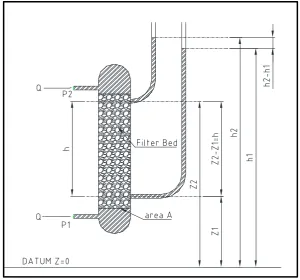
Probably one of the best known models of flow through porous media is Darcy’s law. Darcy's law was derived from experiments performed by Darcy in 1856 on laminar flow through homogenous porous media. The mathematical relationship (Equ 2.5.1) derived from the experiment is:
In this equation Q is the volume flow rate, K is a constant that depends on the properties of the fluid and the porous media. In figure 2.5.1 the layout of Darcy's experiment can be seen, the height h is the characteristic length of the porous media. The difference in height, h2-h1, is
Figure 2.5.1: Darcy's experiment (Scheidegger 1963, p. 70).
Darcy's law has been tested many times showing that it is valid for a wide range of flow domains for liquids and gases. It has also been shown however that Darcy's law is invalid for flow of liquid at high velocity and for gas at both very low and very high velocity. It is believed that Darcy's law breaks down due to the onset of turbulence. This has led to the search for a critical Reynolds number to predict the transition from laminar to turbulent flow. However Scheideeger (1963, p. 169) believes that the breakdown of Darcy's law at high flow rates, is due more to the onset of inertial effects in laminar flow, than that of turbulence. The constant K in Darcy’s law as mentioned is related to the properties of the porous media. One of the most significant properties is that of the permeability of the porous media.
2.6
Porous media and Permeability
A general definition of porous media may be taken as a solid that contains numerous pores or voids. In order for flow to take place within a porous medium some of the pores must be interconnected somehow. The actual shape of these pores is a very difficult thing to define and it is even harder to model these pores mathematically.
In equation 3.1 given previously, the constant K is related to the permeability of the porous media for a particular fluid. The constant K is therefore linked to the two properties; the liquid and the porous media. In order to make better use of Darcy's law the property of permeability needs to be defined. There are numerous equations that attempt to define the permeability of the porous media and therefore separate the effect of the liquid and the porous media that is contained in the constant K.
Another expression (Equ 2.6.1) that is related to permeability is porosity of the filter medium (Horvath 1994, pp. 173-4):
This is the ratio of the total pore volume, in the filter medium, to the total volume of the filter medium. Sand will typically have a porosity value of .
2.7
Filtration Theory
Filtration through porous media is thought to occur by a combination of the following transport processes (Binnie et al. 2002; Horvath 1994):
Interception
Diffusion
Hydrodynamic effect
Inertia
Attachment
These transport processes are shown in figure 3.2 which shows a suspended solid particle as it interacts with a grain of porous media.
Figure 3.2: Various transport processes related to filtration (Horvath 1994, p. 178).
Interception shown figure 3.2a occurswhen the particle in the fluid is intercepted by the filter medium. This is not to be confused with straining, which occurs when large particles are blocked by the filtrate. Rather interception is able to capture much smaller particles than would be possible with straining. Interception works by the adhesion of the particle to the surface of the filtrate medium.
Diffusion (figure 3.2b) is due to Brownian motion that affects very small particles, 1 micron or less, in the fluid flow. The path of the small particles is altered causing collision with the filtrate media. The number of collisions that occur has been said to be proportional
to , where T is equal to temperature, being the diameter of the particle, being the diameter of the filter media, and being the velocity of the flow. The importance of this transport process is also thought to be low.
Hydrodynamic effect (figure 3.2e) or action occurs when a particle in the fluid passes a grain of filter media. The particle then rotates into the filter media as a result of velocity gradients. The particle will then attach to the filter media. This effect is not considered to be too
Inertia effect (figure 3.2c) in water filtration basically involves the collision of particles with the filter media. This will occur as long as the particle is not overcome by the hydrodynamic effects that would see the particle turn and pass by the filter media.
Attachment (settling figure 3.2d) of particles to filter media occurs usually because of Van der Waal's forces between the filter media and the particle being filtered. This will occur provided that there are no electrostatic forces repelling the particle from the filter media. If particles are electrically charged then attachment will only occur if the electrostatic forces are opposite.
The various transport mechanisms given above will occur simultaneously, in varying degrees, in practical filtration. The relative importance of the individual transport mechanisms will vary depending on particle size being removed. It has been noted that the important transport mechanism for very small particles, in the order of , is diffusion. And for particles in the order of size the important transport mechanism is interception. Finally for larger particles, in order of and above, the predominant transport mechanism is straining (Binnie et al. 2002, p. 146). In summary interception and diffusion are of the most
importance in practical filtration, the mechanism of straining is considered to lead to poor filtration efficiency.
2.8
Water Channelling in Porous Media
The channelling of fluids in porous media is experienced in many areas of science and
engineering. In the oil industry channelling of fluids in porous media has an adverse effect on the recovery of oil from wells (Salazar-Mendoza & Espinosa-Paredes 2009; Zhao 2011). Water channelling is quite simply the tendency of the water to flow along the path of least resistance. In a porous media this could be an area of decreased density in relation to the remainder of the structure.
In a horizontally orientated sand filter the effect of water channelling occurs along the top of the filter. This was noted by Mossad & Aral (2010, p. 287) when investigating solutions to the water channelling in water filtration. The water channel is indicated by a small air gap that occurs when water is added to compacted filter sand.
Water channelling can also occur at other layers in a porous medium. This has been observed in experiments of subsurface flows. In these experiments the inlet and outlet positions of a horizontal sand filter were varied to study the effects of water channelling (Suliman et al. 2006). The filter medium was also varied from a homogenous glass bead to layered packing of various sizes. Water channelling was noted to occur readily in the porous media of various sizes. This can be attributed to the density gradients created by the size difference in the grains of the porous media.
2.9
Summary
Water treatment is an important part of the health and well being of society, sand filtration plays an important part in water treatment and therefore health. The delivery of treated water by the lowest economic means is an important priority for both developed and developing countries.
Several general classifications of sand filter are used in modern water treatment plants; horizontal sand filters are currently used as roughing filters. Horizontal sand filtration through pipes could be an economical alternative when a solution to the limitation of water channelling is found.
The most used equation that describes the behaviour of fluids through porous media is Darcy’s law. It is valid for flows of fluid at low velocity and becomes invalid when the velocity becomes excessive. It is applicable at the velocities that are commonly used in water filtration.
In order to use Darcy’s law in practice the permeability of the porous media must be
modelled so that it can be applied to a range of fluids. The relationship between pores in sand filters is very complex; therefore idealised models are needed to describe the relationship. Filtration through porous media relies on several attachment theories to explain the removal of particles from the fluid. The importance of the theory depends on the size of the particles that are to be removed by the porous media. Interception and diffusion are the most important theories used in modern water treatment.
Chapter 3
M ETHODOL OGY
3.1
Introduction
The methodology that will be used for this project will be to numerical model and optimise the layout of the spiral baffle using CFD software. Software simulation was used as it
allowed for multiple variations of the spiral geometry to be checked in a fast and economical fashion.
The CFD analysis consists of several components needed to be able to successfully to model flow in a horizontal sand filter. The components are; the numerical method, the governing equations, creation of the geometry, modelling of the water channel region and calculation of the residence time.
3.2
Numerical Methods for Porous Media
For modelling flow through porous media the equation generally used is that derived from Darcy’s law. As discussed earlier this law holds for low filtration rates with flows in the laminar region only. For turbulent flow through porous media other models must be used. The Reynolds number can be used in order to determine the flow regime that could be expected from a given filter loading rate. The critical Reynolds number, that defines the transition from laminar flow to turbulent flow in porous media has been given as Rcrit =38 (Horvath 1994, p. 177). Some caution should be used when applying a critical Reynolds number as the value will vary depending on the theory of permeability used. Scheidegger (1963, pp. 158-60) reported a large discrepancy amongst authors in regards to the critical value of Reynolds number at which the Darcy equation would no longer hold. None the less the calculation for Reynolds number (Equ 3.2.1) is:
However when the flow is through a porous media then the equation (Equ 3.2.2) changes to (Binnie et al. 2002, p. 141):
f is the porosity of the media.
D is the particle diameter.
is the velocity into the filter.
is the viscosity.
This calculation will be used to check the flow regime through the filter prior to solver setup. An alternative to the Reynolds number, which is reportedly more commonly used with
The Blake number is essentially a modified Reynolds number with terms that take into account the nature of the porous media. The Blake number (3.2.3) is given by:
v v With the hydraulic radius (Equ 3.2.4) equal to:
Using equation 3.2.4 in equation 3.2.3 gives:
v Which reduces to give a Blake number equation of:
v v
= filtration rate (m/h).
= thickness of the filter medium.
= particle diameter (mm).
= pore volume.
= hydraulic radius.
v = kinematic viscosity (mm2/s).
The term S in equation 3.2.6 is the specific surface area of the media in the filter per unit volume, this relationship is:
In order to use equation 3.2.2 the permeability must be calculated for the porous region. The permeability is calculated in FLUENT™(ANSYS FLUENT User's Guide 2010, p. 301) using the Blake-Kozeny equation (Equ 3.2.8) as follows:
This is similar to the equation (Equ 3.2.9) used by Mossad & Aral (2010, p. 288) for permeability calculations which was given as:
When solving porous media flow problems using FLUENT™ the pores of the media are considered to be 100% open. The software FLUENT™ defines the porosity as the open volume fraction of the media being used.
3.3
Governing Equations
The governing equations that are used in (ANSYS FLUENT User's Guide 2010) to model water flow through the porous media are the continuity and momentum equations. Given the assumption of incompressible laminar flow, constant viscosity, and the effects of gravity, the following equations can be derived:
The above equations represent the continuity (Equ. 3.3.1) and momentum equations (Equ. 3.3.2, 3.3.3, 3.3.4) and including the source term S for porous media. The source term, as given in the FLUENT™ user guide, gives a pressure drop caused by the resistance to flow due to the presence of the porous media (sand) that is proportional to the fluid velocity. The equation is given as:
The first term in the above equation is Darcy's law, viscous loss term, and the second is the inertial loss term.
In equation 5.3 above represents the inertia resistance factor, is the permeability of the porous media. When the flow is laminar the inertial resistance term can be ignored which will leave Darcy's law to be included.
The source term in equation 5.4 now represents the pressure drop given in Darcy’s law:
The velocity that will be used in the model of the sand filter will be chosen after review of the literature and the past experiments of Mead (2009) and Mossad & Aral (2010). In Mead’s work on the optimisation of vertical baffles in a horizontal sand filter a loading rate of 0.005m/s was used. This loading rate is similar to that used for the filtration of water in a rapid sand filter described by (Binnie et al. 2002). Mossad & Aral (2010, p. 288) on the other hand used 0.01m/s which is a much greater loading rate than that used for rapid sand
3.4
Model Geometry
To be able to carry out CFD analysis on the spiral baffled filter then the geometry of each case must be modelled. The geometry for CFD needs to be of a good quality, this will make meshing of the models much easier. In this case ANSYS Design Modeller was used; the basic geometry was derived by creating a cylinder and removing the spiral baffle with a sweep feature by invoking the pitch command.
The spiral baffle variables that will be changed are the pitch of the baffle and the height of the baffle. The various combinations of baffle height and pitch that will be used are shown in table 3.2 below. A minimum of three baffle heights and pitches will be used; any less than this would not allow for any meaningful results as trends will not show up. More models would allow for even better resolution of results but time constraints dictate the use of no more than nine models.
Figure 3.1: Spiral baffle filter geometry.
In addition to these models a plain filter was also modelled that has no baffle. The plain filter that will be designated SF10 is used as a base line and to look at the flow through a sand filter without baffles. The overall length and diameter of the geometry is the same as the other filters given in figure 3.1 above.
Model Numbers for Various Baffle Configurations Pitch H=0.02m H=0.04m H=0.06m
0.25m SF01 SF02 SF03
0.35m SF04 SF05 SF06
0.45m SF07 SF8 SF9
3.5
Modelling the Water Channel Region
Modelling the water channel is an important part of being able to model the behaviour of the flow in the horizontal sand filter. As mentioned in problem description the phenomena of water channelling is the very thing that makes horizontal sand filtration undesirable. For this reason the water channel region must be recreated in the model to be able to assess the ability of any proposed solution.
For the examination of the spiral baffle solution the following method has been used to create the water channel. The software allows the user to define a function (UDF) for any of the variables that are input into Fluent. The UDF that was used to model the water channel in this case has three assumptions.
[image:29.595.77.519.357.637.2]The first assumption is that the water channel region occupies only the top 5% of the volume within the horizontal filter. This is the same assumption that has been used by Mossad & Aral (2010, p. 228) and Mead (2009) in their analysis of horizontal baffled filters. So for the sake of being able to compare results this assumption is being used here. This assumption would benefit from more empirical data relating to the exact nature of the water channel region at the top of the filter.
Figure 3.2: Filter cross section showing variation of viscous resistance as percentage of volume.
The second assumption that has been made in regards to the water channel region relates to the value of the low resistance path. The lower resistance has been created by making it three orders of magnitude lower than that of the viscous resistance. This approach is consistent with that used by both Mossad & Aral (2010) and Mead (2009) in their Analysis.
Water Channel 5% Volume at 4.89e6 m-2 Viscous Resistance
This approach is also recommended by the software manufacturer for the application (ANSYS FLUENT User's Guide 2010, pp. 228-9).
The third assumption is that there is a clear demarcation between the two resistance zones within the filter. The performance of the porous media, in this case sand, at this transition point may not behave as a porous material. For it to fit the definition of porous material it must be immoveable and the pores are continuous (Scheidegger 1963, pp. 5-8). However if a great enough velocity exists at the transition point then the sand may percolate within the low resistance zone. The transition zone assumption will therefore need to be validated at some stage in the future.
For the purpose of this analysis the aforementioned assumptions will be held and applied to the CFD models. The UDF that has been created for the viscous resistance will apply these assumptions to each of the equations within the solver. For details of the UDF refer to appendix C.
3.6
Calculating Residence Time
Calculation of residence time will be used to help optimise the spiral baffle geometries that have been modelled. The residence time will be used to give a relative comparison, between the selected geometries, of the time taken for a particle to traverse the filter.
The software offers several options for calculating the residence time; these options depend on the multiphase model being used. The method used with the Eulerian multiphase model is the used by Mossad & Aral (2010, p. 290). The method starts with the use of a two phase model, the second phase is named tracer and is given properties identical to that of the first phase which is water. A volume fraction of 10% of the tracer phase is defined at the inlet boundary of the spiral baffled filter. The modelled is then solved for a transient state and the facet average of the tracer at the outlet boundary is monitored. The flow time taken for the 10% of the tracer to appear at the outlet boundary is recorded as the residence time.
This method will allow for the comparison of each model in relation to the residence time, it does not however give any indication of the filtration efficiency. The reason for this is that the filtration attachment mechanisms, such as interception, are not accounted for. If the attachment mechanisms were accounted for then the model may well be suitable for very basic filtration efficiency calculations through the use of residence time.
3.7
Summary
All nine spiral baffle models will have the same velocity, porous and viscous resistance inputs. The value for the porosity that has been chosen was identified through the literature review. The porosity in each case will be 0.35 which is at lower end of the range given in the literature as between 0.35 to 0.45.
The viscous resistance, which will be discussed further in the solver setup, has been
3.1 below the permeability is first calculated. The diameter of the media used for modelling porous media is 0.55mm in diameter which coincides to a grade of sand typically used in a rapid sand filter. The permeability is calculated thus:
Equation 3.1:
The viscous resistance is the inverse of the permeability that has just been calculated, which is:
Equation 3.2:
Chapter 4
COMPUTATION AL FLUID DYNAMICS SETUP
4.1
Introduction
An important part of the performance of a CFD analysis is the setup of the software to solve the given flow problem. In this case the setup must allow the methodology to be used to find the solution. The models and solver used will now be presented as they relate to the spiral baffle sand filter. The details of the meshing will also be presented here as it is closely related to the performance of the solvers in finding the solution.
4.2
Boundary Conditions
The boundary conditions used to model the spiral sand filters are the same for each case studied. The boundary conditions used to model the spiral sand filter include the following:
Inlet
Outlet
Wall (Including baffle)
Bulk (Internal area)
4.1.1
Inlet Conditions
The inlet boundary condition has been set to velocity and gauge pressure. The value of the velocity used is 0.01m/s which have been identified in the literature as rate similar to that used in a horizontal pressure filter.
The pressure at the inlet is considered to be gauge pressure zero which indicates atmospheric pressure.
4.1.2
Outlet Condition
The outlet condition for the spiral filter model is that of pressure gauge. The outlet of the spiral filter is considered to empty to atmosphere and therefore has a pressure of zero set.
4.1.3
Wall and Baffle Boundary Conditions
The wall of the spiral baffled sand filter is defined at the outer surface of the cylindrical filter body plus the baffle wall. The conditions at the wall are considered to be a non-slip condition. All nine spiral baffle models will have the same velocity, porous and viscous resistance
inputs. The value for the porosity that has been chosen was identified through the literature review. The porosity in each case will be 0.35 which is at lower end of the range given in the literature as between 0.35 to 0.45.
The viscous resistance, which will be discussed further in the solver setup, has been
4.1 below the permeability is first calculated. The diameter of the media used for modelling porous media is 0.55mm in diameter which coincides to a grade of sand typically used in a rapid sand filter. The permeability is calculated thus:
Equation 4.1:
The viscous resistance is the inverse of the permeability that has just been calculated, which is:
Equation 4.2:
The viscous resistance in equation 4.2 will be used to model the resistance in the sand of the horizontal filter. The area of the filter that is taken up by the water channel will be of a lower resistance however and will need to be set to a lower value.
4.3
Selection of CFD Model
The selection of the model for solving the problem needed to consider the calculation of the residence time in addition to the pressure drop and the velocities. The residence time would be calculated using a volume fraction technique and this would determine the model used. A multiphase model would be used which would give access to various methods of calculating residence time for a volume fraction of water.
The Eulerian model was chosen as it uses a set of equations for each phase, these equations are coupled by a common pressure value. This method gives very accurate results but is also more computationally expensive, meaning the solution will take longer to achieve.
Some of the limitations of the Eulerian model are:
The Reynolds stress turbulence model is not available.
Particle tracking interacts with primary phase only.
Inviscid flow is not allowed.
Due to the flow through the filter being laminar none of the limitations affect the modelling of the spiral baffled filter.
4.4
Selection of Solver
The solver type that has been used the CFD analysis of the spiral baffle filters is a pressure based solver. This type of solver is suitable for incompressible flows so is well suited to the anticipated flow through the sand filter.
The other reason for the use of the pressure based solver is the multiphase models that are available with it. The multiphase model will be used in the residence calculation as discussed previously in the methodology.
The algorithm used for the "Phase Coupled SIMPLE" is adapted from the well known SIMPLE scheme and couples both phases with a single pressure. The SIMPLE scheme provides a way of calculating the pressure and velocity for the flow. This is required as the assumption of
incompressibility of flow leaves no independent pressure equation in the governing equations (Tu et al. 2008, pp. 163-5).
The Phase Coupled SIMPLE scheme solves velocities in a segregated way that is coupled to each phase. The pressure correction is created from the momentum equations of each phase and the total continuity of the flow (ANSYS FLUENT User's Guide 2010, pp. 1190-3). The phase coupled scheme is robust and has been used for solving multiphase flows in ANSYS Fluent™ for many years.
4.5
Meshing of Spiral Filter
All the spiral baffled filters have been meshed using the same method; however each filter has a different number of nodes and elements. The variation in nodes and elements between the filter models is due to the variation in meshable area found in each geometry.
The elements used in the mesh are tetrahedrons which are applied using a patch conforming method available in the software.
Models Elements Nodes Ave. Skewness STD Deviation
SF01 1.257e6 3.235e5 0.26299 0.135
SF02 1.192e6 3.165e5 0.24466 0.137
SF03 7.655e5 2.317e5 0.24663 0.141
SF04 4.317e5 1.219e5 0.26021 0.132
SF05 2.884e5 84547 0.27521 0.138
SF06 2.456e5 75241 0.27959 0.146
SF07 2.523e5 81610 0.27875 0.138
SF08 5.669e5 1.775e5 0.21743 0.140
SF09 99320 37142 0.26565 0.151
SF10 101569 44026 0.17339 0.118
Chapter 5
M ODEL RESULT S
5.1
Introduction
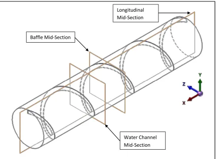
[image:36.595.74.514.308.632.2]The results of the CFD analysis for each of the nine models will be presented focusing on the pressure drop, velocity profile and the residence time. An interpretation of the results will proceed and an attempt made to isolate an optimal configuration for the cases presented. Presentation of the velocity profiles has been considered at two positions, the baffle mid-section and the water channel mid-mid-section. The water channel mid-mid-section is at a position half way between the pitch of the baffles (refer figure 5.1.1). This will give a plane that is equal distance between the baffles as they cut through the water channel. The baffle mid-section is directly aligned vertically with the baffle as it cuts through the water channel (refer figure 5.1.1).
Figure 5.1.1: Orientation of planes used for reporting velocity.
These planes will differ from those used by Mossad & Aral (2010) in their comparison of various baffle options. Mossad & Aral(2010) used a section that was midway between the inlet and outlet of the filter. If this middle section was chosen for the spiral baffle models used in this investigation then the velocity profiles would change, due to the position of the plane in relation to the baffle (refer figure 5.1.2). The baffle position would vary for each different pitch, therefore making comparison more difficult between the various models.
Water Channel Mid-Section Longitudinal Mid-Section
`
Figure 5.1.2: Baffle position at Mid-Section plane in relation to the water channel. The pressure contours and velocity vectors will be presented in Appendix B along the longitudinal mid-section (figure 5.1.1) in each case. The baffle velocities will also be presented in Appendix B; the results are of less use in regards to comparing the various models due to the nature of the flow around the baffle.
The water channel midsection results give a good comparison between the various models, as the plane cuts the channel the same way in each case. The velocity results along the x, y and z axis will be presented for each case. A general discussion of the flow characteristics will be given as the behaviour of the flow in all models showed significant similarity.
Water Channel
Baffle Position SF02 0.25 Pitch
Baffle Position SF05 0.35 Pitch
5.2
General Flow Characteristics
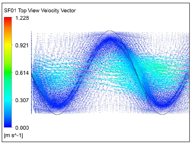
The flow through all the models of spiral baffle showed similar characteristics. The most obvious characteristic is the high flow in the water channel region which can be seen in figure 5.2.1 below. Details of the magnitude of this flow will be given in following sections.
[image:38.595.136.460.217.450.2]The flow around the baffle where it cuts through the water channel can also be seen in figure 5.2.1 below. In this case the flow is shown along the mid-plane of the filter; the flow pattern clearly shows the water flowing downward, under the baffle and up the other side.
Figure 5.2.2: Velocity vectors top view, 0.25m pitch and 0.02m baffle height.
The velocity along the z-axis is in the negative direction, this is the opposite direction to that indicated by the velocity vectors at the top of the filter (figure 5.2.2). The reason for this is that the flow along the z-axis at the bottom of the baffle flows towards the low pressure side of the baffle. So at the bottom of the baffle it effectively flows backward as this is the shortest path to the lower pressure side of the baffle.
Figure 5.2.3: Velocity baffle mid-section of SF01, 0.25m pitch and 0.02m baffle height. -0.2
-0.1 0 0.1 0.2 0.3 0.4
-0.1 -0.08 -0.06 -0.04 -0.02 0 0.02 0.04 0.06 0.08 0.1
V
el
oc
it
y
(m
/s
)
Vertical Distance along the baffle middle line (m)
Baffle Velocity X, Y and Z Axis
[image:39.595.74.513.439.730.2]Velocity along the y-axis stayed fairly neutral until just below the baffle. At this point there was some rapid change between positive and negative values. The negative flows are a sign that the flow is moving downward, this is to be expected given the water is flowing around the baffle (refer figure 5.2.1).
5.3
Water Channel Velocity Results.
The velocity results in the water channel, for all the filter models, will be presented along each axis separately. The reason for this is the large variation in velocity between the x-axis and that of the y-axis and z-axis which makes plots difficult to interpret otherwise.
The velocity results will also be presented in table form showing the peak velocity and position as well as the average velocity.
5.3.1
Results of Velocity X-Axis
All the velocities along the x-axis at the water channel mid-section show the same pattern. As expected the velocity sharply increases as it enters the water channel at approximately 0.08m height (figure 5.3.2). At the bottom of the filter the velocity drops to zero at a position that corresponds to the height of the baffle for the particular filter model.
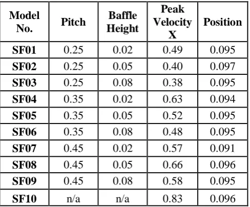
The peak velocities along the x-axis for each filter are given in table 5.3.1 below. From this it is clear that the position at which the peak velocity occurs within the water channel for each filter model is approximately the same.
The magnitude of the peak velocities is considerably higher than the inlet velocity of the filter which is 0.01m/s. This is not unexpected given that the resistance in the water channel is several orders of magnitude less than the remainder of the filter.
Model
No. Pitch
Baffle Height
Peak Velocity
X
Position
SF01 0.25 0.02 0.49 0.095 SF02 0.25 0.05 0.40 0.097 SF03 0.25 0.08 0.38 0.095 SF04 0.35 0.02 0.63 0.094 SF05 0.35 0.05 0.52 0.095 SF06 0.35 0.08 0.48 0.095 SF07 0.45 0.02 0.57 0.091 SF08 0.45 0.05 0.66 0.096 SF09 0.45 0.08 0.58 0.095
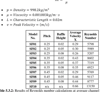
[image:41.595.177.421.434.636.2]The Reynolds number for the average flow velocity in the channel section of the filter should be considered given the large increase in velocity. The characteristic length that will be used for the calculations is the depth of the low resistance channel. The formula used is:
Model
No. Pitch
Baffle Height
Average Velocity
X
Reynolds Number
SF01 0.25 0.02 0.29 5798 SF02 0.25 0.05 0.30 5989 SF03 0.25 0.08 0.26 5207 SF04 0.35 0.02 0.43 8602 SF05 0.35 0.05 0.37 7319 SF06 0.35 0.08 0.35 6923 SF07 0.45 0.02 0.29 5769 SF08 0.45 0.05 0.46 9117 SF09 0.45 0.08 0.44 8777
[image:42.595.85.427.145.460.2]SF10 n/a n/a 0.66 13150
Table 5.3.2: Results of Reynolds number calculations at average channel velocity. The calculated Reynolds number at the inlet velocity is:
Figure 5.3.3: Mid water channel velocity along the x-axis for all filters.
5.3.2
Results of Velocity Y-Axis
The results of velocity along the y-axis (figure 5.3.5) at the mid-section of the water channel show much lower velocities which is to be expected. From the velocity vectors (Appendix B) it can be seen that the flow is predominately along the x-axis. The filter models show a mix of negative and positive velocity in the water channel region. The negative velocity is an indication of flow in a downward direction. This mix of positive and negative velocities is more apparent when looking at tables 5.3.4 and 5.36.
Model
No. Pitch
Baffle Height
Peak
Velocity Y Position
SF01 0.25 0.02 -0.0058 0.090
SF02 0.25 0.05 0.0020 0.086
SF03 0.25 0.08 0.0026 0.099
SF04 0.35 0.02 -0.0018 0.091
SF05 0.35 0.05 -0.0036 0.092
SF06 0.35 0.08 -0.0058 0.087
SF07 0.45 0.02 0.0013 0.093
SF08 0.45 0.05 0.0108 0.090
SF09 0.45 0.08 -0.0042 0.088
SF10 n/a n/a -0.0046 0.086
Table 5.3.4: Peak velocities along y-axis in water channel for all filter models. 0 0.1 0.2 0.3 0.4 0.5 0.6 0.7 0.8 0.9
-0.1 -0.08 -0.06 -0.04 -0.02 0 0.02 0.04 0.06 0.08 0.1
V el oc it y (m /s )
Distance along the section middle line
Mid Channel Velocity X
The position at which the peak velocity occurs in each filter is approximately the same and equates to a point that is midway in a vertical direction.
Figure 5.3.5: Mid water channel velocity along the y-axis for all filters.
The average velocities in the water channel (table 5.3.6) show no real pattern in relation to the pitch of baffle height. The average velocity in the water channel of the filter without the baffle, SF10, is small in magnitude and negative indicating a downward flow.
Model
No. Pitch
Baffle Height
Average Velocity Y
SF01 0.25 0.02 -0.0035
SF02 0.25 0.05 0.0006
SF03 0.25 0.08 0.0011
SF04 0.35 0.02 0.0001
SF05 0.35 0.05 -0.0023
SF06 0.35 0.08 -0.0035
SF07 0.45 0.02 0.0004
SF08 0.45 0.05 0.0054
SF09 0.45 0.08 -0.0027
SF10 n/a n/a -0.0021
Table 5.3.6: Average velocities y-axis in water channel for all filter models. -0.02 -0.015 -0.01 -0.005 0 0.005 0.01 0.015
-0.1 -0.08 -0.06 -0.04 -0.02 0 0.02 0.04 0.06 0.08 0.1
V el oc it y (m /s )
Distance along the section middle line
Mid Channel Velocity Y
5.3.3
Results of Velocity Z-Axis
The velocity results along the z-axis are similar to the results from the y-axis velocities. The similarities are that there is a mix of both positive and negative velocities and that the magnitude of the velocities is low.
Figure 5.3.7: Mid water channel velocity along the z-axis for all filters.
The negative velocity in this case indicates that the flow is going in the opposite direction to that of the rotation of the spiral. The position for peak velocity (table 5.3.8) is higher amongst all the filter models, with the values being very close to the boundary layer.
-0.08 -0.06 -0.04 -0.02 0 0.02 0.04 0.06 0.08 0.1 0.12 0.14
-0.1 -0.08 -0.06 -0.04 -0.02 0 0.02 0.04 0.06 0.08 0.1
V el oc it y (m /s )
Distance along the section middle line (m)
Mid Channel Velocity Z
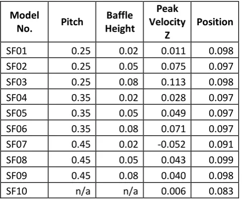
Model
No. Pitch
Baffle Height Peak Velocity Z Position
SF01 0.25 0.02 0.011 0.098
SF02 0.25 0.05 0.075 0.097
SF03 0.25 0.08 0.113 0.098
SF04 0.35 0.02 0.028 0.097
SF05 0.35 0.05 0.049 0.097
SF06 0.35 0.08 0.071 0.097
SF07 0.45 0.02 -0.052 0.091
SF08 0.45 0.05 0.043 0.099
SF09 0.45 0.08 0.040 0.098
SF10 n/a n/a 0.006 0.083
Table 5.3.8: Peak velocities along z-axis in water channel for all filter models.
The average velocity in the water channel is very low in magnitude, which is again expected due the predominance of the velocity along the x-axis. The average in most cases is much greater than the filter without a baffle. This is not too surprising as the flow in the spiral baffle filter should have a tendency to follow the curve of the baffle, therefore making flow along the z-axis much greater.
Model
No. Pitch
Baffle Height
Average Velocity
Z SF01 0.25 0.02 -0.0015
SF02 0.25 0.05 0.0127
SF03 0.25 0.08 0.0342
SF04 0.35 0.02 0.0016
SF05 0.35 0.05 0.0055
SF06 0.35 0.08 0.0166
SF07 0.45 0.02 -0.0308
SF08 0.45 0.05 0.0022
SF09 0.45 0.08 0.0076
[image:46.595.177.421.71.273.2]SF10 n/a n/a 0.0015
5.4
Residence Time Results
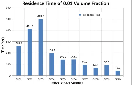
The residence time results, presented in the graph below (figure 5.4.1), shows the residence time for each filter in seconds. The results show that at a pitch of 0.25m there is an increase in the residence time as the baffle height increases. Remembering that SF01 is of 0.02m, SF02 is 0.05m and SF03 is 0.08m in baffle height.
[image:47.595.74.526.247.540.2]The first three filters show the pattern that is expected, as the resistance to flow increases so too does the time it takes for fluid to traverse the filter. The residence times of the other filters are in contrast to this expected behaviour.
Figure 5.4.1: Change in pressure from inlet to outlet for various filter models.
For filters with a pitch of 0.35m the residence time drops from 198.3 seconds for a 0.02m baffle height to 140.5 seconds for the middle baffle height of 0.05m. The residence time for the 0.35m pitch between the 0.05m to the 0.08m baffle height actually increases slightly. This is the same pattern as that of the 0.045m pitch filters but is in contrast to that of the 0.25m pitch filters.
The increase in the residence time of the 0.25m filters as the baffle height increases makes sense. As the baffle height increases the resistance to flow increases and the water is pushed further down into the filter by the baffle. The reason for the decrease in residence time with increased baffle height of 0.35m and 0.45m pitch is unclear.
264.3
411.7
498.6
198.3
140.5 142.0
95.7
69.5 93.3
42.7 0 100 200 300 400 500 600
SF01 SF02 SF03 SF04 SF05 SF06 SF07 SF08 SF09 SF10
T im e (s ec )
Filter Model Number
Residence Time of 0.01 Volume Fraction
One possible explanation is the effect of increasing pitch; this may well exceed the effect that a change in baffle height has on the residence time. This would explain why there is a large drop between 0.25m pitch and 0.35m pitch and a continued drop of smaller magnitude to 0.45m pitch.
The other possible explanation is error in the method used to calculate the residence time. The volume fraction method used a transient solver and the time step was varied to different degrees throughout the solution process. The time steps were altered to reduce solution time but may well have introduced some error to the calculations.
5.5
Pressure Drop Results
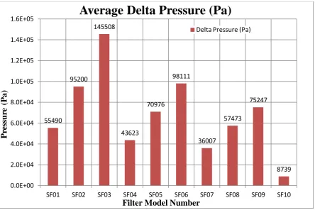
[image:49.595.77.522.192.488.2]The pressure drop across the filter for each model can be seen in the graph below (figure 5.5.1), with the baffle height and pitch for each case given in table 5.5.2. The pressure drop increases as the baffle height increases for each case of pitch. Filters with the greatest baffle height of 0.08m are SF03, SF06 and SF09. These filters show the greatest pressure drop in comparison to filters of the same pitch.
Figure 5.5.1: Change in pressure from inlet to outlet for various filter models.
As the pitch increases the pressure drop can be seen to decrease for all filters of the same baffle height. For example the filter models SF03, SF06 and SF09 show a decrease in pressure drop as the pitch goes from 0.25m, for SF03, to 0.45m for SF09.
Model Number Pitch (m) Baffle Height (m)
SF01 0.25 0.02
SF02 0.25 0.05
SF03 0.25 0.08
SF04 0.35 0.02
SF05 0.35 0.05
SF06 0.35 0.08
SF07 0.45 0.02
SF08 0.45 0.05
SF09 0.45 0.08
SF10 n/a n/a
Table 5.5.2: Filter model numbers showing pitch and baffle height. 55490 95200 145508 43623 70976 98111 36007 57473 75247 8739 0.0E+00 2.0E+04 4.0E+04 6.0E+04 8.0E+04 1.0E+05 1.2E+05 1.4E+05 1.6E+05
SF01 SF02 SF03 SF04 SF05 SF06 SF07 SF08 SF09 SF10
P re ss u re ( P a)
Filter Model Number
Average Delta Pressure (Pa)
The significance of the pressure drop across the filters is apparent when the change in pitch and the change in height are considered separately.
Figure 5.5.3: Change in pressure as pitch increases at different baffle heights.
In figure 5.5.3 the pitch is varied for all three cases of baffle height. In each case as the pitch increases the pressure drops for the same baffle height.
In a similar fashion the baffle height was varied and the pressure change plotted for each case of pitch. This can be seen in figure 5.5.4 on the following page. As the baffle height is
increased from 0.02m through to 0.08m the pressure increases for each case of filter pitch. y = 212525x2 - 246184x + 103753
R² = 1
y = 536095x2 - 563903x + 202670 R² = 1
y = 1E+06x2 - 1E+06x + 371333 R² = 1
0.0E+00 2.0E+04 4.0E+04 6.0E+04 8.0E+04 1.0E+05 1.2E+05 1.4E+05 1.6E+05
0.2 0.25 0.3 0.35 0.4 0.45 0.5
P
re
ss
u
re
(
P
a)
Pitch (m)
Pressure Change With Pitch
Pressure Drop for 0.02m Height
Pressure Drop for 0.05m Height
Figure 5.5.4: Change in pressure as baffle height increases at different baffle heights.
In each case the pressure drop is much greater than the filter without a baffle, SF10. The only resistance in SF10 is that of the porous media and so can be considered as the base line for all other models.
The change in pressure with pitch and baffle height mean that there are many possible combinations of baffle height and pitch that could give the same pressure drop. This will be discussed further when the subject of optimisation is discussed.
y = 6E+06x2 + 911552x + 34904 R² = 1
y = -120777x2 + 920204x + 25268 R² = 1
y = -2E+06x2 + 859129x + 19645 R² = 1
0.0E+00 2.0E+04 4.0E+04 6.0E+04 8.0E+04 1.0E+05 1.2E+05 1.4E+05 1.6E+05
0 0.01 0.02 0.03 0.04 0.05 0.06 0.07 0.08 0.09
P
re
ss
u
re
(
P
a)
Baffle Height (m)
Pressure Change With Baffle Height
Pressure Drop for Pitch 0.25m
Pressure Drop for Pitch 0.35m
5.6
Filter Power Input Calculations
The power input required by each filter is to be used to compare results and for optimisation in regards to residence time. The power in watts will be calculated for each filter model using the volume flow rate and pressure drop as follows:
The results of the power input calculation for each filter model are given in table 5.7.1 below. Model
Number
∆p (Pa) Q (m3/s) P (W)
SF01 5.55E+04 3.12E-04 17.32 SF02 9.52E+04 3.12E-04 29.67 SF03 1.46E+05 3.10E-04 45.17 SF04 4.36E+04 3.12E-04 13.60 SF05 7.10E+04 3.10E-04 22.02 SF06 9.81E+04 3.09E-04 30.31 SF07 3.60E+04 3.12E-04 11.22 SF08 5.75E+04 3.12E-04 17.91 SF09 7.52E+04 3.09E-04 23.23
SF10 8.74E+03 3.12E-04 2.73
Figure 5.6.2: Chart showing spiral filter input power for various models.
The chart in figure 5.6.2 shows a definite pattern in regards to the change in power required for the various filters. Looking at a particular baffle height such as 0.02m height which covers models SF01 (pitch 0.25), SF04 (pitch 0.35) and SF07 (pitch 0.45) you can see the power required drops as pitch increases.
Focusing on the change in baffle height as the pitch remains the same the inverse occurs. For example models SF01 (Baffle 0.02m), SF02 (Baffle 0.05m) and SF03 (Baffle 0.08m) the power required increases from 17.32 Watts for SF01 to 45.17 Watts for SF03. As expected all filter models require more power input than the non-baffled filter SF10.
These changes in power required make sense when considering the baffles and the resistance that they have to flow through the filter. The resistance to flow in relation to the pitch will decrease as the pitch increases. This is due to the decreasing angle the baffle takes to the flow along the x-axis. The change in angle of the baffle in relation to the x-axis can be seen in figure 5.6.3 below showing SF01 of pitch 0.25m and SF07 of 0.45 pitch.
17.32 29.67 45.17 13.60 22.02 30.31 11.22 17.91 23.23 2.73 0 5 10 15 20 25 30 35 40 45 50
SF01 SF02 SF03 SF04 SF05 SF06 SF07 SF08 SF09 SF10
P owe r (W at ts )
Filter Model Number
Spiral Sand Filter Input Power (Watts)
Figure 5.6.3: Spiral baffle SF01 of 0.25m pitch compared to SF07 of 0.45m pitch.
The resistance will increase as the baffle height increases as obstruction to the flow will be greater for the larger baffle height. This can be visualised by examining the velocity vectors in figure 5.6.4 which shows SF01 and SF03 which are at the extremes of baffle height for a pitch of 0.25m.
Figure 5.6.4: Velocity vectors for SF01 and SF03 showing of flow around baffle.
5.7
Optimisation of Results
The discussion of optimisation will start with a discussion of the various results that will be used. The pressure drop across the filter is one of the more important results that will be used. The residence time data will also be looked at for its suitability in the optimisation of the spiral baffled filters.
The results of the pressure drop and the power calculation show a definite relationship between the baffle height, pitch and the pressure drop. The relationship however of the baffle height and the pitch is not such that a single optimal solution can be found. Instead the two variables can be changed in value to adjust the power required. The use of a performance chart is one way to optimise the selection of baffle height, pitch and power required.
Figure