Shape optimization of metallic yielding devices for passive mitigation of seismic energy

Shape optimization of metallic yielding devices for

passive mitigation of seismic energy

Kazem Ghabraiea, Ricky Chanb,∗, Xiaodong Huangb, Yi Min Xieb

a_{Faculty of Engineering and Surveying, University of Southern Queensland, Toowoomba Qld}

4350, Australia

b_{School of Civil, Environmental and Chemical Engineering, RMIT University, GPO Box 2476,}

Melbourne VIC 3001, Australia

Abstract

Bi-directional Evolutionary Structural Optimization (BESO) is a well established

topology optimization technique. This method is used in this paper to optimize

the shape of a passive energy dissipater designed for earthquake risk mitigation.

A previously proposed shape design of a steel slit damper (SSD) device is taken

as the initial design and its shape is optimized using a slightly modified BESO

algorithm. Some restrictions are imposed to maintain simplicity and to reduce

fabrication cost. The optimized shape shows increased energy dissipation capacity

and even stress distribution. Experimental verification has been carried out and

proved that the optimized shape is more resistant to low-cycle fatigue.

Keywords: Shape optimization, Energy dissipation, Bi-directional Evolutionary

Structural Optimization, Metallic damper, Cyclic tests, Earthquake resistant

structure

∗_{Corresponding author}

Email addresses:[email protected](Kazem Ghabraie),

1. Introduction

In the last two decades development of energy dissipation devices for

miti-gation of wind and earthquake has flourished. Various types of passive,

semi-active and semi-active devices have been proposed, tested and implemented [1]. With

this technology, a large portion of input energy from wind or earthquake

exci-tations is dissipated by designated devices. As a result, structural responses are

suppressed, and major structural elements can be protected from damage.

Particu-larly in earthquake applications, metallic devices which utilize yield deformation

of metals remain among the most popular types selected by engineers. They are

reliable, inexpensive to fabricate, easy to install and maintain. Metallic devices

can be classified into flexural types, such as hourglass shape ADAS [2],

triangu-lar shape TADAS [3]; shear types such as YSPD [4] and axial types, such as the

Buckling Retrained Brace [5]. Devices are mainly designed to be incorporated

into lateral-load-resisting system in structural frames, but some are developed to

be installed between beam and columns [6].

Design of metallic devices requires several desirable engineering

characteris-tics:

1. possessing sufficient elastic strength and stiffness such that device is not

excited to inelastic region under service loads;

2. having stable and large energy dissipative capability; and

3. having reasonable resistance against low-cycle fatigue.

With respect to low-cycle fatigue, current design standard in the United States

requires devices to undergo five fully reversed cycles at maximum earthquake

de-vice displacement (ASCE/SEI 7-05). Generally, in order to increase the resistance

Along with the revolutionary improvement of digital computers in recent decades,

computational methods and numerical techniques have established their place as

invaluable engineering tools. Among these, numerical optimization methods have

attracted a great number of researchers and have been improved a lot. Particularly,

the state-of-the-art shape and topology optimization techniques have been applied

to a range of physical problems and have been proved to yield much better results

than experimental designs [8, 9]. The Evolutionary Structural Optimization (ESO)

method, introduced by Xie and Steven [10] is a simple and effective topology

op-timization technique which can tackle shape opop-timization problems as well. This

method iteratively improves the design domain by removing its inefficient parts.

A Bi-directional version of the ESO method, called BESO, has been later

pro-posed by Querin et al. [11, 12] and Yang et al. [13]. In BESO, besides removal

of inefficient parts, the efficient parts of the design domain will be improved by

adding more material next to them. Since its introduction, the BESO algorithm

has been improved significantly [14]. The improved BESO algorithm has been

successfully applied to non-linear problems [15, 16]. This method is also capable

of optimizing both shape and topology of the designs [17].

In this paper, the BESO algorithm is modified to optimize the shape of an

ex-isting steel slit damper device design (SSD). The proposed algorithm applies some

shape restrictions to the design to make the final shape easily manufacturable. An

efficient device design should possess a high energy dissipation capability per unit

volume. To gain this, the proposed algorithm maximizes the total plastic

dissipa-tion. It is also demonstrated that the optimum design resulted from the proposed

optimization algorithm, show less stress concentration than the initial design.

numerical models, physical experiments are carried out. It is demonstrated that

experimental outcomes support the numerical results.

2. Optimization

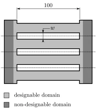
Chan and Albermani [18] have proposed a class of simple designs for SSD

devices supported by a series of experimental test results. Fig. 1 shows the typical

shape of the device. The size of the slits (w) can be controlled by varying land

b. In this paper, a new class of design is proposed by optimizing the shape of

the slits in Fig. 1. To achieve this, a shape optimization algorithm based on the

BESO technique is proposed and utilized here. Some restrictions are imposed to

maintain the simplicity of the shape and hence reduce its fabrication costs. These

restrictions are discussed in detail in Section 2.4.

Figure 1: The SSD device design proposed by Chan and Albermani [18].

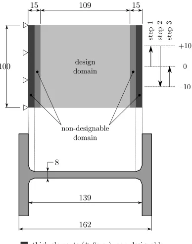
2.1. Numerical modeling

For numerical modeling, the flanges are considered solid and a plane stress

is considered overall the design except for the elements on the far left and right

sides of the domain. These elements which are in the vicinity of the flanges are

modeled using thicker elements to simulate fillets (Fig. 2).

For the sake of fabrication, the holes are prevented from being too wide by

setting the two strips of 15mm width on the left and right sides as non-designable

elements. Fig. 2 illustrates the designable and non-designable domains.

The left side of the model is fixed and a uniform vertical displacement is

ap-plied to the right side of the model. The loading cycle consists of three steps: an

upward displacement of 10mm, followed by a downward displacement of 20mm,

and finally an upward displacement of 10mm up to the original location (Fig. 2).

In this manner the elastic strain energy will be zero after a full cycle and the total

strain energy would be equal to the total plastic dissipation.

2.2. Problem statement

To optimize the shape of the SSD, the total plastic energy dissipation is

con-sidered as the objective function which is to be maximized. In order to prevent the

optimization algorithm from catching the extreme full or empty domain designs,

it is necessary to include an additional constraint to restrict the amount of usable

material [19]. Here we use a volume constraint which forces the algorithm to use

a certain amount of material in the design domain. Alternatively, one can impose

a restriction on the maximum force instead of using a volume constraint [15]. The

optimization problem can be expressed as

max

x1,x2,...,xN

EP

subject to V =V¯

and shape restrictions

whereEPis the total plastic dissipation;Vand ¯Vare the actual and target volumes;

xi-s are the design variables andNis the number of elements in the design domain.

Shape restrictions are fully covered in Section 2.4. In the BESO algorithm, design

variables are binary values with x = 1 indicating the presence of material in the

i-th element andx= 0 representing a void in the location of thei-th element.

2.3. Sensitivity analysis

To evaluate the effect of adding or removing an element during the

optimiza-tion process, one needs to perform a sensitivity analysis.

Because the loading sequence consists of a full cycle, the total plastic

dissipa-tion will be equal to the total strain energy. Hence, for this case, we can write

EP = ET =

I

f·du, (2)

whereET is the total strain energy; andf anduare nodal force and displacement

vectors respectively. Using the trapezoidal method for numerical integration, this

definition can be rewritten as

EP = lim n→∞        1 2 n X

i=1

uT_i −uT_i−1(fi+fi−1)

     

. (3)

The shape sensitivities of the nonlinear systems have been calculated for diff

er-ent types of problems by Huang and Xie [16], Buhl et al. [20], Jung and Gea

[21]. Here we briefly describe the sensitivity analysis of the problem (1) based on

Huang and Xie [16].

To solve the non-linear equilibrium system, an iterative procedure is

com-monly used to eliminate the residual force. The residual force vector,r, is defined

as the difference between the external and internal force vectors. The equilibrium

can thus be expressed as

The internal force vector ˆf is defined as

ˆ

f =

N

X

e=1

Z

Ve

CT_eBTσdV =

N

X

e=1

CT_ep_e (5)

with Ce denoting the matrix that transforms the local nodal values of the e-th

element to global nodal values; B being the matrix that transforms a change in

displacement into a change in strain; and σrepresenting the local element stress

vector.

In order to calculate the sensitivities of the objective function,EP, with respect

to a design variable, x, we rewrite the (3) by adding an adjoint vectorλmultiplied

by a zero function

EP = lim n→∞        1 2 n X

i=1

uT_i −uT_i−1(fi+fi−1)−λ

T

i (ri+ri−1)

     

. (6)

Now, differentiating (6) with respect to x, one can obtain

∂Ep

∂x = nlim→∞ "

1 2

n

X

i=1

uT_i −uT_i−1 ∂fi

∂x +

∂fi−1

∂x ! + 1 2 n X

i=1

∂uT i

∂x −

∂uT_i−1

∂x

!

(fi+fi−1)

−λT_i ∂ri ∂x +

∂ri−1

∂x

!# . (7)

The system of concern is subject to a gradual change in displacement at certain

nodes. At those degrees of freedom where the displacement is explicitly defined,

∂uj

∂x = 0. Everywhere else, fj = 0. The second term in the above equation, thus,

cancels out. Further, by considering (4), the above equation can be simplified to

∂Ep

∂x = nlim→∞ "

1 2

n

X

i=1

uTi −u T i−1

∂fi

∂x +

∂fi−1

∂x

!

−λT_i ∂fi ∂x +

∂fi−1

∂x

!

+λT i

∂ˆ_fi

∂x +

∂ˆ_fi−1

∂x

To eliminate the unknown terms in (8), the adjoint equation is defined as

λi = ui−ui−1 (9)

from which the adjoint vector is readily calculable. Now, using (9) in (8), one can

get

∂Ep

∂x = nlim→∞ "

1 2

n

X

i=1

uT_i −uT_i−1 ∂ˆfi

∂x +

∂ˆ_fi−1

∂x

!#

. (10)

The validity of this sensitivity analysis is demonstrated through a simple analytical

problem by Huang and Xie [16].

Using a linear approximation, one can write

∂EP

∂x ≈ ∆EP

∆x (11)

and

∂ˆ_f

∂x ≈ ∆_fˆ

∆x. (12)

Now using (12) and (11) in (10), the change in the energy dissipation due to a

change in a design variable can be approximated as

∆Ep ≈ lim n→∞ " 1 2 n X

i=1

uT_i −uT_i−1 ∆ˆfi+ ∆ˆfi−1

#

. (13)

From (5), the change in the internal force due to removing or adding an element

can be calculated as

∆_fˆ_{= ∆xeC}T

epe (14)

which can be substituted into (13) to yield

∆Ep≈ ∆xe lim n→∞ " 1 2 n X

i=1

uT_i −uT_i−1CT_e (p_e)i+(pe)i−1

#

Using the trapezoidal numerical integration method and noting the definition of

the dissipated energy in (2), the above equation can be simplified as

∆Ep ≈∆xe lim

n→∞[(Ee)i−(Ee)i−1]= ∆xeEe, (16)

where (Ee)i is the total strain energy of thee-th element after iiteration through

solving the nonlinear equilibrium; and Ee is the final strain energy of the e-th

element upon completion of the loading cycle. Noting the definition of design

variables from Section 2.2, one can observe that for removing an element ∆xe =

−1 and for introducing an element∆xe = +1.

Based on (16) we define the following sensitivity number for an elemente

αe =

∆EP

∆xe

= Ee (17)

which is a measure of efficiency of the e-th element. Note that the sensitivity

numbers defined in (17) are always positive. Remembering that the maximum

value of EP is desirable and noting that ∆EP = αe∆xe, for removing an element

(∆xe = −1), the element with the lowest sensitivity is the most suitable candidate

for removal. On the other hand, introducing a new element strengthens the

adja-cent elements and results in∆xe >0. Hence, in this case, the new element should

be added in the neighborhood of the elements with higher sensitivity numbers.

2.4. Shape restrictions

BESO is naturally a topology optimization method which can introduce new

holes and fill the current holes in the domain. To prevent the algorithm from

changing the topology of the domain and restrict it to shape optimization, it is

slits. In other words, the elements are only allowed to be removed from and added

to the boundary line. The designable domain in each iteration is thus redefined as

D={e|∃i, j∈ B:i, j∈e∧i_, j}, (18)

whereBis the set of boundary nodes defined as

B= {j|∃em ∈ M,ev ∈ V: j∈em∩ev} (19)

withMandVrepresenting the sets of solid and void elements.

2.4.1. Periodicity

In order to enhance the manufacturability of the solutions, a periodic cellular

design is considered with four identical cells similar to the initial SSD design.

The BESO method has been previously proved useful in producing optimal

peri-odic structures [22]. To deal with periperi-odic design problems, the design domain

should be divided into a number of identical cells. The sensitivity numbers of

corresponding elements in all of these cells are then averaged and this averaged

value is used as the sensitivity number for all of these elements. This procedure

can be illustrated as

αi =

1

Ncell Ncell X

j=1

αi,j, (20)

whereαi is the averaged sensitivity number of thei-th element in all cells;αi,j is

the (original) sensitivity number of thei-th element in the j-th cell; andNcellis the

number of cells. In this manner, the BESO algorithm treats all the cells identically

and maintains the periodicity of the design.

2.4.2. Mirroring

Because of the non-linear nature of the problem, the loading sequence will

optimal shape. Hence one would get mirrored shape results if once considers a

displacement cycle starting with an upward moving (↑↓↑) and once with an initial

downward moving (↓↑↓). In real case, however, it is uncertain which direction

is more likely to happen. It is thus reasonable to consider both of these loading

cases. To do so, one should consider the mechanical responses of the two load

cases and add them up together to obtain the correct sensitivity number. However,

as the loading sequences are just mirror reflections of each other, we just need to

add the sensitivities of mirrored elements together. This can be mathematically

expressed as

¯

ai = ai +a↔

i (21)

where ¯ai is the corrected (mirrored) sensitivity number of thei-th element; and

↔

i

is the element at the same location as thei-th element in the mirrored structure.

2.5. BESO procedure

As already mentioned in Section 2.3, the elements with the lowest sensitivity

numbers are the least efficient and should be removed while the ones with

high-est sensitivity numbers are the most efficient and should be strengthened. In the

BESO procedure strengthening the elements is via introducing new elements in

their vicinity. In the new BESO algorithm [14], a filtering scheme is used to assign

a sensitivity number to the void elements in the vicinity of solid elements. The

filtering scheme is a wighted averaging which can be expressed as

ˆ

αi =

PN

j=1α¯jwi j

PN j=1wi j

, (22)

where ˆαi is the filtered sensitivity number of the i-th element andwi j is a linear

weighting factor defined as

HereR is a positive scalar value known as filtering radius anddi j is the distance

between the centroids of thei-th and j-th elements.

Using this filtering scheme, the void elements in the neighborhood of the

ele-ments with higher sensitivity number will obtain higher filtered sensitivity

num-bers. Hence, in the BESO procedure, the void elements with the highest filtered

sensitivity numbers can be assumed as the most efficient choices for introduction

to the system. This filtering scheme also smooths the jagged boundary lines and

overcomes some numerical instabilities such as checkerboard formation [23].

2.5.1. Adding and removing elements

In the optimization problem (1), the volume is fixed to a predefined value, ¯V.

Starting from a feasible design withV = V¯, one needs to add and remove a same

amount of material to keep the volume unchanged. Using identical elements to

discretize the designable domain, the number of adding and removing elements

should be equal. If a solid element has a lower sensitivity number than a void

element, the two elements should be switched. However, in order to prevent

sud-den changes, the maximum number of changes should be restricted. The limiting

number of changes is referred to as ‘move limit’ hereafter and is denoted by m.

Comparing with the BESO algorithm proposed by Huang and Xie [14], the move

limit used here is equivalent to the maximum adding ratio, i.e.m=ARmax.

The optimization loop continues until the following condition is met

Pl i=1E

(k−i+1)

P −E

(k−i)

P

Pl i=1E

(k−i+1)

P

< τ, (24)

where E(_Pi) denotes the value of the objective function at i-th iteration; k is the current iteration number;τis the convergence tolerance selected as 10−4here; and

2.6. Numerical results

The initial design is depicted in Fig. 3. A series of tests are conducted with

different material volumes. Table 1 summarizes the test cases and their

specifica-tions.

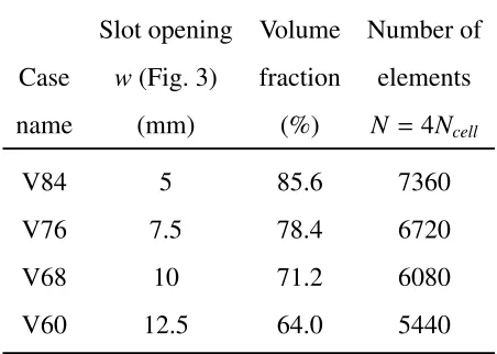
Table 1: The specifications of test cases.

Slot opening Volume Number of

Case w(Fig. 3) fraction elements

name (mm) (%) N =4Ncell

V84 5 85.6 7360

V76 7.5 78.4 6720

V68 10 71.2 6080

V60 12.5 64.0 5440

In all cases the volume is kept constant so that the objective function values for

different iterations could be compared. The move limit is chosen asm= 0.005N.

The number of elements, N, for each case is reported in Table 1. This relatively

small value is adopted due to the small number of elements in the design domain

which is limited to the boundaries of the holes. The filtering radius is selected

as 5mm through all the tests. The initial and final cell designs and the evolution

of the objective functions (energy dissipation) for the test cases are illustrated in

Fig. 4 to Fig. 7.

The increasing trend of the energy dissipation through optimization iterations,

which can be observed in all cases, verifies the proposed approach. It can be

seen that in all cases, the energy dissipation increases significantly. In these four

96% compared to the energy dissipation capability of the initial designs. Table 2

summarizes the improvements in the energy absorption capacity of the test cases.

In order to achieve a simple manufacturable shape, some shape restrictions

have been enforced to the shape optimization problem. Restricting the designable

domain to the small setDdefined in (18) to maintain the topology, forcing the

de-sign to be periodic, and mirroring will all impose limitations to the optimization

process by making its feasible space smaller. Furthermore because of the binary

nature of the BESO algorithm, the feasible space in not continuous. This

re-stricted, discrete feasible space causes some oscillations in the objective function

values observable at the end of the optimization procedures, when the solution is

going to converge.

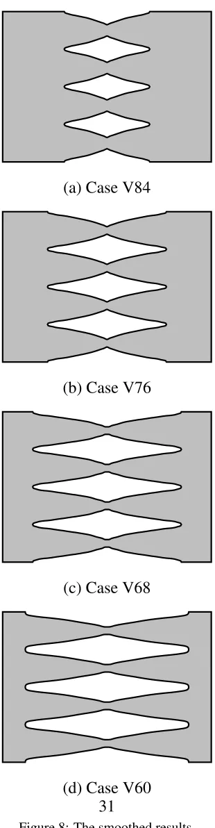
In all cases the optimum cell design is tapered in the middle. As these four

cases had different material volume, it can be concluded that for this sort of

dampers the diamond shaped holes provide the best energy dissipation capacity

irrespective of the material volume.

Table 2: The improvement of the energy dissipation of the test cases after optimization.

EP (J)

Case name Initial Final Improvement (%)

V84 1124. 2203. 96

V76 863. 1440. 67

V68 631. 1000. 58

2.7. Postprocessing

In order to remove the jagged boundaries of the resulted shapes and reduce

the stress concentration it is necessary to smooth the boundaries of the resulted

shapes. A postprocessor is written to automatically smooth the boundaries of the

optimal shapes using B´ezier curves. Fig. 8 shows the smoothed results. It can

be seen that irrespective of the volume fraction, all the optimum shapes include

diamond shaped holes.

To check the effect of the shape optimization on stress distribution, the smoothed

optimal shape of the case V60 is tested against its smoothed initial shape. The

force-displacement curve and the stress distribution of the initial and optimal

shapes are depicted in Fig. 9 and Fig. 10 respectively.

It can be seen in Fig. 9 that the optimum shape provides a stiffer design

com-pared to the initial shape. After undergoing 10mm of displacement, the initial

shape produces a reaction of 16.4kN while the reaction generated in the optimal

shape is 24.3kN. Also a comparison between the stress levels in Fig. 10 reveals

that the optimal shape provide a much evener stress distribution. The stress

con-centration zones in the corner of the holes visible in the initial design are

elim-inated in the optimal shape. The stress concentration zones are prone to fatigue

and undesirable brittle failure under cyclic loads. The fatigue failure of the SSD

devices at these zones have been reported in Chan and Albermani [18].

2.8. Optimal design

Based on the shape optimization results and Fig. 8, three specimens with the

shape design depicted in Fig. 11 are fabricated. These specimens are used for

experimental tests as discussed in the following sections. Because of the tapered

3. Experimental verification

The objective of the experiments is to verify the cyclic characteristics of the

optimized shape. Furthermore, strength-degradation and low-cycle fatigue

char-acteristics of the device are not predicted by the current finite element model.

They must be investigated by physical experiment.

3.1. Test setup, instrumentation and loading history

Identical setup with previous tests [18] was used such that comparable results

could be obtained. The test setup is shown in Fig. 12. The specimens were

in-stalled between a ground beam and an L-beam, securely fastened by four M16

bolts (snug tight) on each side. Forced displacement was applied by an MTS

100kN capacity computer-controlled actuator quasi-statically to the specimen via

the L-beam. To ensure the verticality of the applied load, a pantograph system

was welded to the right hand side of the L-beam. The pantograph system also

pre-vented the L-beam from deflecting out-of-plane. The complete test setup rested

on a reaction frame which was significantly stiffer. The centerline of the

actua-tor implied an eccentricity to the specimen, measured 162mm to the centerline

of the specimen. A free-run of the setup (i.e. without the specimen installed)

was performed and the result showed that friction and the effect of gravity were

considered negligible. The setup was robust and repeatable, no visible damage

occurred after all tests were carried out. Fig. 13 shows a photograph of the setup

with specimen installed.

Displacements of the specimens were measured independently by a pair of

LVDTs, marked as 1 and 2 in Fig. 12. While LVDT 1 measures the elastic

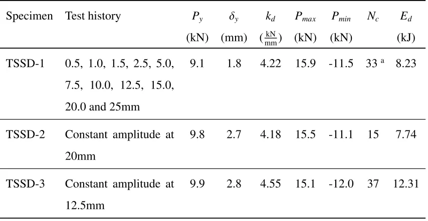
Table 3: Specimens and test results.

Specimen Test history Py δy kd Pmax Pmin Nc Ed

(kN) (mm) (_mmkN) (kN) (kN) (kJ)

TSSD-1 0.5, 1.0, 1.5, 2.5, 5.0,

7.5, 10.0, 12.5, 15.0,

20.0 and 25mm

9.1 1.8 4.22 15.9 -11.5 33a _8.23

TSSD-2 Constant amplitude at

20mm

9.8 2.7 4.18 15.5 -11.1 15 7.74

TSSD-3 Constant amplitude at

12.5mm

9.9 2.8 4.55 15.1 -12.0 37 12.31

a _{Note: TSSD-1 did not break after 33 cycles were completed.}

distortion of the test specimen.

Specimen TSSD-1 was tested under identical displacement history with

pre-viously study on SSD [18]. The load history comprised three repeated cycles at

amplitudes of 0.5, 1.0, 1.5, 2.5, 5.0, 7.5, 10.0, 12.5, 15.0, 20.0 and 25mm.

TSSD-2 and TSSD-3 were tested under a constant displacement until complete breakage

of the specimens. Table 3 summarizes the test histories and key results.

3.2. Specimens

Based on the result of optimization, three specimens were fabricated.

Di-mensions are shown in Fig. 11. All specimens (each 100mm long) in this study

were cut from the same structural wide-flange section 152×152×37 Universal

Column to BS4449 (depth × flange width× web thickness× flange thickness is

is identical and material strengths of all specimens may be assumed equal. Four

16mm diameter holes were drilled on each flange for connection to the test rig.

Two standard test coupons were taken from the web of the section. Coupon tests

gave an average tensile yield stress of 316.5N/mm2 and an average Modulus of

Elasticity of 206.1kN/mm2.

3.3. Test results and discussion

All three specimens deformed in a stable manner under the cyclic tests. The

strips deformed in double curvature as expected. Fig. 14(a) to (c) present the

force-displacement hysteresis obtained from the cyclic tests. A positive sign refers

to downward force and displacement. Shear strain γ (i.e. distortion divided by

total width of device) of the specimens are also shown. Positive yield strengthPy,

its corresponding yield displacementδy, elastic stiffnesskd, positive peak strength

Pmax, negative peak strength Pmin, the number of cycles to failureNc and energy

dissipationEd are tabulated in Table 3.

It is clear that all specimens have yielded at small displacement and exhibited

very stable hysteretic behavior with a gradual transition between the elastic and

inelastic regime. The specimen response magnitude was slightly lesser than the

input displacement history due to elastic deformation of the support. Absolute

displacements (difference across LVDT 1 and 2) are used to determine the

me-chanical properties of the specimens. The connection of the specimens by four

structural bolts on each flange performed satisfactory; no significant distortion

was observed after the tests. Fig. 15 shows the damaged specimen TSSD-1 after

3.4. Specimen TSSD-1

TSSD-1 completed all cycles without breakage. At the end of the 25mm

cy-cle, force was released such that the specimen was left deformed. A photograph

of the specimen after all cycles is shown in Fig. 15. Its force-displacement

hys-teresis is shown in Fig. 14(a). Very stable hyshys-teresis without noticeable sign of

strength deterioration was observed. Cracks have developed on the bar surfaces

due to repeated loading, but they did not cause breakage. Initial yield strength and

displacement were recorded at 9.1kN and 1.8mm respectively. Bauschinger effect

was apparent, with negative peak strength only 72% of the positive peak.

TSSD-1 dissipated 8.23kJ at the end of the cycles. Energy dissipation of

TSSD-1 is shown in Fig. 16. Result from specimen SL-1 [18] is plotted on the

same chart for comparison. To account for different volume of steel involved in

specimens, energy is expressed as energy dissipated per unit volume of steel. Here

the volume of steel between fillets is taken into consideration as the flange does

not contribute to energy dissipation. There is a 37% increase in energy

dissipa-tion and it is evident that the optimizadissipa-tion process has resulted in a more efficient

design. From the same diagram it is clear that, after optimization, TSSD-1

sus-tained a much larger cumulative displacement compared to SL-1. The enhanced

resistance against low-cycle fatigue is clear.

3.5. Specimens TSSD-2 and TSSD-3

TSSD-2 and TSSD-3 were fabricated to identical dimensions as TSSD-1, but

these two specimens were tested under constant amplitudes until complete

break-age. They enable us to identify their energy dissipating capacity under different

displacement amplitudes. TSSD-2 was tested at 20mm (µ ≈ 11) while

in Fig. 14(b) and (c). Both specimens exhibited stable behavior without

notice-able degradation during their early cycles. TSSD-2 sustained 15 complete cycles

prior to failure, while TSSD-3 sustained 37 cycles. TSSD-2 dissipated 7.74kJ of

energy, while TSSD-3 dissipated 12.31kJ. It is interesting that at relatively low

displacements, the device dissipated a much larger amount of energy.

4. Conclusion

This paper proposed a new steel slit damper design, TSSD, based on the

nu-merical shape optimization results. A previously proposed steel slit damper, SSD,

with straight uniform slit width has been taken as the initial design. An

optimiza-tion procedure has been proposed based on the well-known BESO method to find

the optimum shape of the slits. Some shape restrictions have been introduced and

imposed in the optimization procedure to maintain the topology of the design and

restrict it to a symmetric periodic cellular shape with 4 cells. The plastic energy

dissipation of the damper after one cycle of displacement loading with 10mm

am-plitude has been taken as the objective function. The optimization problem has

been then stated as maximizing the objective function while the material volume

is kept constant and the shape is restricted. Four initial models with similar shape

to SSD has been considered as the initial designs each having a different material

volume. The resulted evolution of the objective function values for all the cases

has shown a significant increase in the energy dissipation capacity verifying the

proposed optimization procedure. Improvements of 58 to 96% in the energy

ab-sorption capacity of the designs have been recorded. The optimum shapes were

all include bars tapered in the middle forming diamond shaped slits irrespective

A postprocessor has been used to smooth the optimum results using B´ezier

curves. It has been demonstrated that the optimum tapered slit design provides

an even stress distribution and the stress concentration noticeable in the initial

straight slit design has been eliminated in the optimum design. This even stress

distribution can significantly improve the behavior of the damper under fatigue.

The finite element model used in the optimization process was not capable of

predicting failure and fatigue of the design. Therefore, based on the optimization

findings, three TSSD specimens were fabricated and put under cyclic tests.

Un-der identical test setup and load history, the TSSD specimen dissipated 37% more

energy per unit volume compared to the previously tested SSD, and significantly

delayed low-cycle fatigue. It should be noted that this figure is not comparable

with the improvements reported on Table 2 because the volume of the original

SSD and the proposed TSSD are not equal. Experiments confirmed that the

op-timization process is robust and it is suitable for future development of energy

dissipaters.

Acknowledgement

Experimental works described in this paper is carried out during an academic

visit to City University of Hong Kong by the second author, supported by the

Research Grant Council of Hong Kong City University RGC 115208.

References

[1] Soong TT, Spencer Jr BF. Supplemental energy dissipation: state-of-the-art

[2] Bergman DM, Goel SC. Evaluation of cyclic testing of steel-plate devices

for added damping and stiffness. Tech. Rep. UMCE 87-10; Department of

Civil Engineering, University of Michigan; Ann Arbor, Michigan; 1987.

[3] Tsai KC, Chen HW, Hong CP, Su YF. Design of steel triangular

plate energy absorbers for seismic-resistant construction. Earthq Spectra

1993;9(1993):505–28.

[4] Chan RW, Albermani F, Williams MS. Evaluation of yielding shear panel

device for passive energy dissipation. J Constr Steel Res 2009;65(2):260–8.

[5] Black CJ, Makris N, Aiken ID. Component testing, seismic evaluation

and characterization of buckling-restrained braces. ASCE J Struct Eng

2004;130(6):880–94.

[6] Koetaka Y, Chusilp P, Zhang Z, Ando M, Suita K, Inoue K, et al. Mechanical

property of beam-to-column moment connection with hysteretic dampers for

column weak axis. Eng Struct 2005;27(1):109–17.

[7] ASCE/SEI 7-05. Minimum Design Loads for Buildings and Other

Struc-tures. ASCE Publications; 2006.

[8] Bendsøe MP, Sigmund O. Topology Optimization - Theory, Methods, and

Applications. Berlin: Springer; 2003.

[9] Xie YM, Steven GP. Evolutionary structural optimization. London:

Springer; 1997.

[10] Xie YM, Steven GP. A simple evolutionary procedure for structural

[11] Querin OM, Steven GP, Xie YM. Evolutionary structural

optimisa-tion (eso) using a bidirecoptimisa-tional algorithm. Engineering Computations

1998;15(8):1031–48.

[12] Querin OM, Young V, Steven GP, Xie YM. Computational efficiency and

validation of bi-directional evolutionary structural optimisation. Comput

Method Appl Mech Eng 2000;189(2):559–73.

[13] Yang XY, Xie YM, Steven GP, Querin OM. Bidirectional evolutionary

method for stiffness optimization. AIAA J 1999;37(11):1483–8.

[14] Huang X, Xie YM. Convergent and mesh-independent solutions for the

bi-directional evolutionary structural optimization method. Finite Elem Anal

Des 2007;43(14):1039–49.

[15] Huang X, Xie YM, Lu G. Topology optimization of energy-absorbing

struc-tures. Int J Crashworthiness 2007;12(6):663–75.

[16] Huang X, Xie YM. Topology optimization of nonlinear structures under

displacement loading. Eng Struct 2008;30(7):2057–68.

[17] Ghabraie K. Exploring topology and shape optimisation techniques in

un-derground excavations. Phd thesis; RMIT University; Melbourne, Australia;

2009.

[18] Chan RW, Albermani F. Experimental study of steel slit damper for passive

energy dissipation. Eng Struct 2008;30(4):1058–66.

[19] Rozvany GI, Querin OM, Gaspar Z, Pomezanski V. Extended optimality in

[20] Buhl T, Pedersen C, Sigmund O. Stiffness design of geometrically

non-linear structures using topology optimization. Struct Multidiscip Optim

2000;19(2):1615–488.

[21] Jung D, Gea HC. Topology optimization of nonlinear structures. Finite Elem

Anal Des 2004;40(4):1417–27.

[22] Huang X, Xie YM. Optimal design of periodic structures using evolutionary

topology optimization. Struct Multidiscip Optim 2008;36(6):597–606.

[23] Sigmund O, Petersson J. Numerical instabilities in topology optimization:

A survey on procedures dealing with checkerboards, mesh-dependencies and

0 5 10 15 20 25 30 35 40 45 1100.

1200. 1300. 1400. 1500. 1600. 1700. 1800. 1900. 2000. 2100. 2200. 2300.

Iteration Obj. Function

0 5 10 15 20 25 30 35 40 45 850.

900. 950. 1000. 1050. 1100. 1150. 1200. 1250. 1300. 1350. 1400. 1450.

Iteration Obj. Function

0 2 4 6 8 10 12 14 16 18 20 22 24 26 600.

650. 700. 750. 800. 850. 900. 950. 1000.

Iteration Obj. Function

0 2 4 6 8 10 12 14 16 18 20 22 24 26 28 420.

440. 460. 480. 500. 520. 540. 560. 580. 600. 620. 640. 660. 680. 700. 720.

Iteration Obj. Function

(a) Case V84

(b) Case V76

(c) Case V68

-20 -15 -10 -5 0 5 10 15 20

-12 -10 -8 -6 -4 -2 0 2 4 6 8 10 12

displacement (mm) force (kN)

(a) initial design

-30 -20 -10 0 10 20 30

-12 -10 -8 -6 -4 -2 0 2 4 6 8 10 12 displacement (mm) force (kN)

(b) optimal design

498.40 436.83 375.25 313.68 252.11 190.54 128.97 67.40 5.83

(a) initial design

486.51 426.83 367.14 307.46 247.78 188.10 128.42 68.73 9.05

(b) optimal design

Figure 10: Comparing the stress distribution of the initial and optimal designs for case V60. The

(a) TSSD-1

(b) TSSD-2

Figure 15: Specimen TSSD-1 after the test.