White Rose Research Online URL for this paper:
http://eprints.whiterose.ac.uk/93050/
Version: Accepted Version
Article:
Green, JA, Grigolo, A, Ronto, M et al. (1 more author) (2016) A two-layer approach to the
coupled coherent states method. Journal of Chemical Physics, 144 (2). 024111-024111.
ISSN 0021-9606
https://doi.org/10.1063/1.4939205
[email protected] https://eprints.whiterose.ac.uk/ Reuse
Unless indicated otherwise, fulltext items are protected by copyright with all rights reserved. The copyright exception in section 29 of the Copyright, Designs and Patents Act 1988 allows the making of a single copy solely for the purpose of non-commercial research or private study within the limits of fair dealing. The publisher or other rights-holder may allow further reproduction and re-use of this version - refer to the White Rose Research Online record for this item. Where records identify the publisher as the copyright holder, users can verify any specific terms of use on the publisher’s website.
Takedown
If you consider content in White Rose Research Online to be in breach of UK law, please notify us by
James A. Green,1,a)Adriano Grigolo,2,b) Miklos Ronto,1,c) and Dmitrii V. Shalashilin1,d) 1)School of Chemistry, University of Leeds, Leeds LS2 9JT, United Kingdom
2)Instituto de F´ısica “Gleb Wataghin”, Universidade Estadual de Campinas, 13083-859, Campinas, SP,
Brazil
(Dated: 18 December 2015)
In this paper a two-layer scheme is outlined for the coupled coherent states (CCS) method, dubbed two-layer CCS (2L-CCS). The theoretical framework is motivated by that of the multiconfigurational Ehrenfest (MCE) method, where different dynamical descriptions are used for different subsystems of a quantum mechanical system. This leads to a flexible representation of the wavefunction, making the method particularly suited to the study of composite systems. It was tested on a 20-dimensional asymmetric system-bath tunnelling problem, with results compared to a benchmark calculation, as well as existing CCS, MP/SOFT and CI expansion methods. The two-layer method was found to lead to improved short and long term propagation over standard CCS, alongside improved numerical efficiency and parallel scalability. These promising results provide impetus for future development of the method for on-the-fly direct dynamics calculations.
PACS numbers: Valid PACS appear here
Keywords: quantum dynamics, trajectory-based methods, coherent states, tunnelling, system-bath, wave-function
I. INTRODUCTION
Multilayer variants of existing numerical methods in multidimensional quantum mechanics offer an increase in flexibility and give better scalability for the de-scription of complex quantum systems. Motivated by the extension of multiconfigurational time-dependent Hartree (MCTDH)1,2 to its multilayer formalism (ML-MCTDH)3–5, Gaussian based methods have already been extended in this direction, and a two-layer approach for the Gaussian-based multiconfigurational time-dependent Hartree (G-MCTDH) has been proposed in Ref. 6. Numerous Gaussian based techniques exist for both semi-classical and quantum propagation. Following the sem-inal work by Heller7 many of those methods represent the wavefunction as a superposition of trajectory guided Gaussian coherent states
|Ψ(t)i=
N X
n=1
An(t)|zn(t)i. (1)
In thez-notation representation of coherent states, anM -dimensional coherent state (CS) is a product of M one-dimensional Gaussian wavepackets: |zi = QM
i=1|z(i)i.
The position representation of these states is
hx|z(i)
i= (γ/π)14e−
γ
2(x−q (i))2+i
~p (i)(
x−q(i))+i
2~p (i)
q(i) (2)
where γ describes the width of the Gaussian and q(i)
and p(i) are the coordinate and momentum in the i-th
a)Electronic mail:[email protected] b)Electronic mail:[email protected] c)Electronic mail:[email protected] d)Electronic mail:[email protected]
dimension. These phase space coordinates are related to the real and imaginary parts of the CS label:
z=
r
γ 2q+
i
~ r
1
2γp (3)
which is motivated by the fact that |zi and z are the eigenvector and eigenvalue of the annihilation operator respectively,
ˆ
a|zi=z|zi ; ˆa=
r
γ 2qˆ+
i
~ r
1
2γp .ˆ (4)
The amplitudes in Eq. (1) are usually represented as a product of an oscillating action exponent and smooth pre-exponential factor,8
An(t) =Dn(t)e
i
~Sn(t). (5)
Several methods exist for guiding the trajectories of the CS basis. Semiclassical methods such as Heller’s frozen Gaussian approximation7 and the Herman-Kluk propagator9–11 use classical trajectories and a semiclas-sical description for the amplitudes. There are also a number of formally exact Gaussian-based methods such as multiple spawning (MS)12,13, coupled coherent states (CCS)8,14–16 and variational multiconfigurational Gaus-sians (vMCG)17,18. These methods use exact quantum equations for the amplitudes An(t) in Eq. (1) but
dif-fer in the way that the basis|zn(t)i is guided. MS uses
purely classical mechanics whereas vMCG relies on com-plicated trajectories obtained from a full variational prin-ciple applied to the complete wavefunction|Ψ(t)i. The fully variational trajectories of vMCG are strongly quan-tum: different basis vectorszn(t) couple to one another,
quantum techniques are reminiscent of classical molecu-lar dynamics (MD) and are capable of representing quan-tum molecular dynamics.
The main advantage of trajectory guided methods is that most of the time the basis set follows the dynami-cally important region, thus economising its size. How-ever, in many cases a small trajectory guided basis is efficient for short time period only. When trajectories in multidimensional phase space run away from each other, even fully variational trajectories become uncoupled and classical. Therefore they become unable to correctly fol-low the dynamics in strongly non-classical degrees of free-dom, misguiding the basis. To address this issue, the multiconfigurational Ehrenfest (MCE)19,20approach was suggested. In the version of MCE proposed in Ref. 20, a regular basis set is used to represent the dynamics in a “more quantum” subsystem instead of a single CS. The Ehrenfest configuration basis takes the form
|ϕn(t)i= (a1n(t)|1i+a2n(t)|2i+. . .
+aKn(t)|Ki)|z(c)n (t)i (6)
where the set of states {|1i,|2i, . . . ,|Ki} represents an orthonormal basis ofKfunctions for the “quantum” sub-system, for example, K electronic potential energy sur-faces like in Ref. 20 or a set of K discrete value rep-resentation (DVR) points. A single Gaussian trajectory guided coherent state,|z(c)n (t)i, describes the “classical”
degrees of freedom. A single Ehrenfest configuration is not flexible enough to describe complicated quantum dy-namics accurately but a superposition of Ehrenfest con-figurations
|Ψ(t)i=
K X
n=1
An(t)|ϕn(t)i (7)
can be converged to a quantum result. As Eq. (7) repre-sents the whole wavefunction as a superposition of Ehren-fest configurations, even “classical” degrees of freedom are represented on a fully quantum level irrespective of the fact that within a given configuration, such as in Eq. (6) they are described by a single CS. Coupling between the coefficientsAn(t) in Eq. (7) ensures that the
trajecto-ries|z(c)n (t)iare weighted according to quantum
dynam-ics. Several versions of MCE exist, and results have been obtained for spin-boson model19, non-adiabatic dynam-ics of pyrazine20, dynamics of adsorption on the surface21 and dynamics of quantum qubits coupled with the elec-tromagnetic field22. Gaussian multiconfigurational time-dependent Hartree (G-MCTDH)23 method also relies on the same idea of using regular MCTDH wavefunctions for a small “quantum” subsystem and Gaussian wavepackets for “classical” degrees of freedom.
In this paper we suggest a variation of MCE, which – instead of a regular basis – uses Gaussian CSs for the “quantum” subsystem. The algorithm, which is termed as two-layer CCS (2L-CCS), is fully trajectory based and
represents quantum molecular dynamics. Many quan-tum techniques, which use the basis of trajectory guided Gaussian CS, have been implemented in Cartesian frame (Cartesian CCS24, MS12,13, MCE25–28, vMCG17,18 on the fly) so that they would work similar to classical MD. A great deal of effort has been invested in the develop-ment of quantum direct dynamics, which uses electronic structure software packages on-the-fly to estimate forces which in turn guide the trajectories and the matrix el-ements of quantum coupling between them.12,13,25–28So far these direct dynamics methods have been focused on electronically non-adiabatic effects. Being a trajectory based method 2L-CCS is well suited to Cartesian frame implementation, and we point out from the outset that the future aim is to implement 2L-CCS in this manner so that it may provide a better description of tunnelling in ab initiodirect dynamics simulations than standard CCS. Throughout the remainder of the paper, atomic units are used with~= 1, and the coherent state parameterγ in
Eq. (2) is set to unity.
II. WORKING EQUATIONS OF TWO-LAYER CCS
A. Wavefunction ansatz
Assuming that the system is comprised of “quantum” and “classical” subsystems we represent the Ehrenfest configuration29–31 as follows:
|ϕn(t)i=
a1n(t)|z(q)1n(t)i+a2n(t)|z(q)2n(t)i+. . .
+aKn(t)|z(q)Kn(t)i
|z(c)n (t)i. (8)
In this equation |z(q)kni = QM(q) i=1 |z
(i)
kni and |z
(c)
n i =
QM
i=M(q)+1|z
(i)
n i are the coherent states covering M(q)
“quantum” and the remaining “classical” degrees of free-dom. The difference between Eqs. (6) and (8) is that in the latter the “quantum” subsystem is represented not on a regular fixed basis set but on the basis of trajec-tory guided CSs. The “classical” subsystem is still rep-resented by a single Gaussian. The total wavefunction is a superposition of configurations:
|Ψ(t)i=
N X
n=1
Dn(t)|ϕn(t)i (9a)
=
N X
n=1
Dn(t) "K
X
k=1
akn(t)|z(q)kni #
|z(c)n (t)i (9b)
=
N X
n=1
Dn(t) "K
X
k=1
akn(t)|zkn(t)i #
. (9c)
“classical” subsystem is treated on a fully quantum level and the ansatz of Eq. (9) is formally exact: it can be converged (at least in principle) to the fully quantum result. It is convenient to introduce full dimensional CS:
|zkn(t)i=|z
(q)
kn(t)i|z
(c)
n (t)i (10)
as in Eq. 9c, bearing in mind that for a given indexnall |zkn(t)iwith different k differ only by their “quantum”
part.
Coherent states are not orthogonal: the overlap be-tween two states is described by the overlap matrix32:
hzkn|zlmi= exp
z∗knzlm− z∗knzkn
2 −
z∗lmzlm
2
. (11)
The matrix elements of the Hamiltonian can be written in coherent state basis by representing the Hamiltonian with creation and annihilation operators in normal order (powers of the creation operator to the left of those of the annihilation operator); the matrix elements become
hzkn|Hˆ|zlmi=hzkn|zlmiHord(z∗kn,zlm), (12)
where in the normal ordered Hamiltonian Hord(: ˆa†,ˆa:)
ˆ
a† and ˆaare simply replaced byz∗ andz respectively.
B. Equations of motion
Time-dependence of the phase space coordinates of the CSs|z(q)kniand|z(c)n i, as well as their corresponding
am-plitudesakn(t) andDn(t), determine the time-evolution
of the wavefunction. The equations of motion can be obtained from a full variational approach by taking (9) as a trial state and optimising all wavefunction param-eters {z(q)kn,z(c)n , akn, Dn} at once. This procedure has
been applied to Gaussian based wavefunctions in Refs. 6, 18, 23, 33, however one can also treat some of the parameters variationally while prescribing the dynamics of the others. Under this scheme, different methods can be used within a single configuration to propagate the “quantum” and “classical” sub-systems. In this work we use predetermined CCS and Ehrenfest type trajecto-ries forzkn andzn respectively, which intuitively follows
from our experience with each method. This is com-bined with variational equations for the amplitudes in each layer which ensures that 2L-CCS is an (in princi-ple) exact technique. It is important to point out that the prescribed CS dynamics is not an approximation, but rather a convenient, simple and stable way of guiding the basis set. Providing the basis set sufficiently covers phase space over the time frame of a calculation, the exact re-sult may be obtained. See for example Ref. 34where the efficiency of guiding the basis by classical and variational trajectories is compared, and both are shown to converge to the same result. The particular prescriptions employed here find their justification in the time-dependent varia-tional principle (TDVP) when it is applied to individual
basis set elements and configurations. The derivation of the working equations which involves using normalisation constraints and appropriate choice of phases for the CS elements, is presented separately in AppendixA.
In the first layer the standard CCS basis equation
˙
z(q)kn =−i∂Hord(z ∗ knzkn)
∂z(knq)∗ (13)
is used to describe the dynamics of “quantum” coordi-nates. As has been discussed in Refs. 8, 14,15 the tra-jectories (13) are classical in nature, although the Hamil-tonian includes quantum corrections. The amplitudes are conveniently written as a product of an oscillating action exponent and smooth pre-exponential factor
akn=dkneiSkn , (14)
with classical action
Skn= Z t
0
i 2(z
∗
knz˙kn−z˙∗knzkn)−Hord(z∗kn,zkn)
dt′.
(15) The equations of motion fordcan be found as
i K X
l=1
hzkn|zlnid˙lneiSln = K X
l=1
hzkn|zlniδ2Hkn,ln′ dlneiSln,
(16) where
δ2Hkn,ln′ =Hord(z∗kn,zln)−Hord(z∗ln,zln)
−i(z∗kn−z∗ln) ˙zln. (17)
This is the same as in the CCS method, the only differ-ence being that the Hamiltonian matrix elements have explicit time-dependence due to the motion of “classi-cal” modes. Equations (13), (15) and (16) constitute the first layer of the two-layer CCS approach.
For the second layer of “classical” degrees of freedom, MCE equations are used for the trajectories:
˙
z(c)n =−i∂hϕn|Hˆ|ϕni ∂z(nc)∗
(18a)
=−i K X
kl=1
d∗
kndlnhz(q)kn|z(q)lni
∂Hord(z∗knzln) ∂z(nc)∗
ei(Sln−Skn).
(18b)
The Ehrenfest trajectories (18) account for the effect of the “quantum” subsystem on the motion of the “sical” subsystem by averaging the Hamiltonian of clas-sical DOF with the wavefunction of “quantum” subsys-tem. The “classical” DOF Hamiltonian itself also in-cludes CCS quantum corrections. Then, upon substitu-tion of the resulting wavefuncsubstitu-tion in the time-dependent Schr¨odinger equation, the equations for the amplitudes of configurations are found to be
i N X
m=1
hϕn|ϕmiD˙m= N X
m=1
h
hϕn|Hˆ|ϕmi −ihϕn|ϕ˙mi i
Dm,
which can be recast in terms of the basic variables as
i N X
m=1
K X
kl=1
d∗
kndlmhzkn|zlmiD˙mei(Slm−Skn)= N X
m=1
K X
kl=1
hzkn|zlmid∗kn
−id˙lm+ ∆2Hkn,lm′ dlm
Dmei(Slm−Skn), (20)
with the coupling matrix ∆2H′ being:
∆2H′
kn,lm=Hord(z∗kn,zlm)−Hord(z∗lm,zlm)−i(z∗kn−z∗lm) ˙zlm. (21)
Thus, the Ehrenfest equations of motion in Eqs. (18) and (20) are used for the trajectories and amplitudes of the “classical” layer. We again emphasise that even the second layer “classical” subsystem is treated on a fully quantum level. The only difference between “classical” and “quantum” levels is that the “classical” system is represented by a single Gaussian and single trajectory per configuration, while the “quantum” subsystem is repre-sented by a more flexible linear combination ofK Gaus-sians per configuration guided by their individual trajec-tories. Similar to the CCS technique, the right hand side of the coupled equations (16) and (20) is small. As has been shown previously (see Refs. 8,14–16,18), matrices δ2H′and ∆2H′are small, sparse and have zero diagonal. It should be noted that the two-layer equations of mo-tion can be simplified by using the fact thathzkn|zlni=
hz(q)kn|z(q)lniand by splitting the action (15) into two parts, one depending on both indicesknand the other depend-ing only on the configuration index n – see Appendix A.
In this section we have described another approach to guide the trajectories of a Gaussian CS basis set. Within a single configuration na small set of “quantum” DOF should be sampled with coherent statesz(q)kn such that all important parts of the phase space of the “quantum” sub-system are covered. Using several CSs per configuration to parametrise the “quantum” subsystem describes quan-tum delocalisation better. The trajectories of “quan-tum” subsystem are given by CCS equations (13) and quantum effects are taken into account via the coupling of their amplitudes (16). The “classical” DOF are de-scribed by a single trajectory, which is influenced by the “quantum” subsystem via the Ehrenfest equation (18). The description of “classical” DOF is less detailed. To account properly for quantum dynamics of the “classi-cal” subsystem the configurations are weighted with their amplitudes (19) and equations for the coupling coeffi-cients are derived. The specific choice of the trajectories (13) and (18), which are almost as simple and computa-tionally inexpensive as classical trajectories ensures the smallness and sparsity of the quantum coupling matrices in Eqs. (16) and (20). In summary, Eqs. (13), (16), (18) and (20) constitute the proposed 2L-CCS approach. If only one CS is used to describe the “quantum” subsys-tem (k= 1 in Eq. (9b)) then 2L-CCS yields the standard
CCS method.
III. IMPLEMENTATION AND RESULTS
A. Hamiltonian
The test system investigated is that of a particle sub-jected to an asymmetric double well potential whose mo-tion is also coupled to a bath; this same system was stud-ied by the matching-pursuit/split-operator Fourier trans-form (MP/SOFT) method35, CCS36 and recently by a trajectory-guided strategy using a configuration interac-tion (CI) expansion of the wavefuncinterac-tion37. The model Hamiltonian
ˆ H =pˆ
(1)2
2 −
ˆ q(1)2
2 +
ˆ q(1)4
16ξ + ˆ P2
2 +
1 +λqˆ(1)ˆ
Q2
2 (22)
isM-dimensional, where (ˆp(1),qˆ(1)) are the position and
momentum operators of the 1D tunnelling (“quantum”) subspace and ( ˆQ,Pˆ) are the position and momentum operators of the (M −1)-dimensional (“classical”) sub-space, with ˆQ = PM
i=2qˆ(i) and ˆP =
PM
i=2pˆ(i). As in
previous works35–37we consider the case of M = 20, set the potential parameterξ= 1.3544 and the system-bath coupling constant λ = 0.1. As the coupling is linear with respect to q(1) and quadratic with respect to Q,
the model describes the case of asymmetric tunnelling, because the coupling with the bath increases the right hand well depth forq(1)<0 and decreases it forq(1)>0.
For the initial state all bath modes are in their harmonic ground states.
For illustrative purposes we also show the equations of motion used in 2L-CCS. If we denotezkn(q) = (q(1)kn + ip(1)kn)/√2 andzn(c)= (Qn+iPn)/
√
2, then the equations for the “quantum” modes read
˙
q(1)kn =p(1)kn (23a)
˙
p(1)kn =−(M−4 1)λ−
3 8ξ −1
−q (1)3 kn
4ξ − λ 2Q
2
while the “classical” modes are governed by
˙
Qn =Pn (24a)
˙
Pn =−Qn−λhϕn|qˆ(1)|ϕniQn, (24b)
withk= 1,2, . . . , K andn= 1,2, . . . , N. The equations (23) and (24) are different from those of classical me-chanics. Most importantly, in the two-layer context the “classical” modes couple with the “quantum” subsystem via the average value of the “quantum” mode position operator ˆq(1) over then-th configuration|ϕ
ni; this
aver-age is explicitly given by
hϕn|qˆ(1)|ϕni
=
K X
kl=1
d∗
kndlnhzkn(q)|z
(q)
ln i
zkn∗(q)+zln(q)
√ 2
!
ei(S(q)ln−S
(q)
kn).
(25)
Clearly, the “quantum” nature of the 1D tunnelling mode makes itself present in the equations of motion for the “classical” (bath) coordinates. This clarifies the funda-mental idea behind the two-layer approach: by taking into account this distinction between the different degrees of freedom at the level of the equations of motion for the “classical” (bath) modes, one hopes to enhance the qual-ity of the configurations|ϕniused to expand the system
wavefunction as in (9), in the sense that the number of configurations needed to converge the results is expected to be minimised.
B. Benchmark calculation
The benchmark calculation relies on the fact that the modes ( ˆQ,Pˆ) are equivalent and thus effectively indistin-guishable. As a result, one may use permutational sym-metry and combine the multidimensional basis functions in groups. The approach is equivalent to second quanti-zation and further details may be found in AppendixB, or Ref. 38 which also contains full results for the model Hamiltonian (22). The benchmark calculations are fully converged for the set of parameters used in this article for Hamiltonian (22).
C. Initial basis set sampling for CCS and 2L-CCS
In a multidimensional system only a basis which is sufficiently compressed and biased to the position of the initial wavefunction |Ψ(0)i in phase space can re-sult in an accurate representation. For the Hamiltonian (22) considered in this work, the initial wavefunction |Ψ(0)i is a multidimensional Gaussian wavepacket with phase space coordinates of the tunnelling mode located at the minimum of the lower well: q(1)(0) = −2.5 and
p(1)(0) = 0.0, whilst initial coordinates of the bath mode
are q(i)(0) = 0.0 and p(i)(0) = 0.0 for i > 1. As has
been shown in Ref. 16the quality of the initial basis can be assessed from the norm of the wavefunction. For a good quality basis, covering densely the phase space re-gion where the whole wavefunction is located, the norm
hΨ|Ψi=
N X
nm=1
D∗
nhϕn|ϕmiDm
=
N X
nm=1
D∗ nDm
K X
kl=1
d∗
kndlmei(Skn−Slm)hzlm|zkni
(26)
becomes close to unity.
For the CCS method, initial random basis set sam-pling of the tunnelling mode and bath modes is centered around the initial tunnelling and bath positions respec-tively, and conducted via a Monte Carlo distribution of the form8
f(z(i))
∝exp(−α(i) |z(i)
−z(i)(0)
|2). (27)
The compression parameter α(i) sets the width of the
distribution in thei-th degree of freedom; the larger the value ofα(i), the more compressed the distribution (this
is merely a sampling parameter and is not connected to the widthγ of the coherent state). Different initial ba-sis set distributions can be used for different types of modes, in this case the tunnelling and bath modes. This is called a “pancake” distribution.16 Sampling for 2L-CCS may proceed in exactly the same way as 2L-CCS, due to the wavefunction ansatz (9) conveniently splitting the basis into “quantum” and “classical” subsystems, allow-ing “pancake” samplallow-ing.
In Ref. 36, for the tunnelling problem (22), a broad distribution was used for the tunnelling (“quantum”) mode and narrow distributions were used for the 19 bath (“classical”) modes. However, the result obtained in that work was in some disagreement to that ob-tained by other methods.35,37 Based on the sampling of MP/SOFT and CI expansion, and results from the benchmark calculation,38 it was established that one of the possible reasons for this is that the bath was insuf-ficiently sampled and a broader distribution is required. Consequently, the CCS calculation will be repeated in this work. However, it is not possible to sample all bath modes from a broad distribution, as this results in CSs that are inadequately coupled. Therefore, drawing on inspiration from the benchmark calculation in which a number of individual bath modes are “excited”, a ran-dom two bath modes per configuration are sampled from a broad distribution (“excited”) with compression pa-rameter αb, whilst all others are sampled with an
infi-nite compression parameter. Both distributions are cen-tred on the initial bath coordinates q(i)(0) = 0.0 and
p(i)(0) = 0.0 for i > 1. This allows the value of αb to
to an appropriate balance of ample bath sampling and well conserved norm near unity; though we admit this is quite an ad hoc approach which is left to be better understood in future investigations. The bath for both CCS and 2L-CCS is sampled in this way.
Increasing the number of configurations N also al-lows the value of αb to be reduced whilst maintaining
a norm close to unity. This effect has been previously demonstrated in Ref. 16and can be applied in the same manner for both CCS and 2L-CCS. For example, when N = 2000 a value of αb = 0.8 was used for both CCS
and 2L-CCS, whilst forN= 100 a value ofαb= 5.0 was
used. TableI compares the initial bath samplings used for various K and N parameters. The tunnelling mode is sampled from a relatively broad distribution around the initial wavepacket coordinates q(1)(0) = −2.5 and
p(1)(0) = 0.0, as in previous work,36 with compression parameterαs= 1.0 for all values ofKand N.
Calculation of the initial amplitudes proceeds in two stages: firstly, the set ofKamplitudes for a given config-urationnare obtained via projection of the initial “quan-tum” coherent state distribution |z(q)kni onto the initial wavepacket for the tunnelling mode|Ψ(q)(0)i
hz(q)ln|Ψ(q)(0)i=
K X
k=1
dkn(0)hz
(q)
ln|z
(q)
kni. (28)
Once the the initialdkn amplitudes have been calculated
for all N configurations, the Dn(0) amplitudes may be
determined by projection of the entire initial coherent state distribution|zknionto the entire initial wavepacket
|Ψ(0)i
hzlm(0)|Ψ(0)i= N X
n=1
Dn(0) K X
k=1
dkn(0)hzlm(0)|zkn(0)i.
(29)
D. Comparison of the 2L-CCS method with standard CCS and against benchmark results
In this section 2L-CCS is compared with standard CCS and against the benchmark calculations for coupling pa-rameter λ = 0.1, for which results from MP/SOFT35 and CI expansion37methods are also available. The CCS results are re-calculated in this work, rather than using those from Ref. 36in view of the improved sampling pro-cedure mentioned in the previous section. In the CCS calculations all modes are governed by the CCS equa-tions (13), (15) and (16,17) with the complete system wavefunction having the form of Eq. (1). In the 2L-CCS calculations, 2L-CCS equations (13), (15) and (16,17) are used for the tunnelling mode only, while the time-evolution of the bath modes is determined by Ehrenfest trajectories (18), which give rise to Eq. (24). Standard CCS with the basis ofN CSs can be regarded as 2L-CCS with N configurations and with a single (K = 1) CS in each configuration.
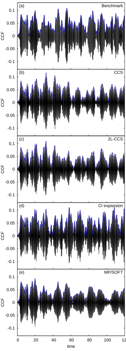
The quantity of interest is the cross-correlation func-tion (CCF) between the wavefuncfunc-tion at timetand mir-ror image of the initial state |Ψ(0)¯ i, i.e. the overlap hΨ(0)¯ |Ψ(t)i. The mirror state coordinates are ¯q(1)(0) =
+2.5 and ¯p(1)(0) = 0.0 with all bath modes coordinates
and momenta set to zero. Since the mirror state is lo-cated in an upper local energy minimum, non-zero values of the CCF are indicative of tunnelling. The power spec-tra, calculated by taking the Fourier transform of the CCF as
I(ω) =
Z T
0
Re[hΨ(0)¯ |Ψ(t)i]e−iωtdt (30)
will also be used for comparisons among the different methods, and is used as an indication of the long-term propagation accuracy. The total propagation timeT = 120 time units for all methods. The comparison of the results from various methods35,37,38 can be seen in Fig. 1 for the cross-correlation function and in Fig. 2 for the Fourier transforms. Both CCS and 2L-CCS cross-correlation functions compare well to the other methods and the benchmark at early time scales (t < 25−a.u.), and the Fourier spectra have peaks of the same frequen-cies and similar intensities. However, the splitting of the peaks in the spectra is not well reproduced by CCS and 2L-CCS, which may be explained by two reasons. Firstly, the basis does not effectively cover the high energy region, hence the high frequency peaks are not faithfully repro-duced. A similar effect was found with CCS when applied to the far infrared absorption spectrum of a water trimer in Ref. 39. Secondly, the splitting of the lower energy peak atω = 9.5 is not as large for CCS and 2L-CCS as it is for the benchmark because it does not begin to ap-pear until 50 a.u. into the benchmark calculation, and by this point Monte-Carlo noise has begun to affect the CCS and 2L-CCS calculations, reducing their accuracy.
The CCS and 2L-CCS calculations can both be con-verged by increasing the number of configurations N, whilst 2L-CCS has the additional flexibility of increas-ing the number of basis vectorsK per configuration for convergence. As 2L-CCS uses a random sampling of basis functions, like CCS it will be plagued by noise inherent to the method and propagation will be most accurate for short time scales, as mentioned above. Therefore for these short time scales we should expect the calculation to converge towards the benchmark result, which is what is shown in Figs. 3 and 4. It can be seen in Fig. 3 that the quality of short-term propagation is affected by the number of basis vectors per configuration: the larger the value of K for the same number of configurations, the better the result. This is illustrated qualitatively in panels (a)–(c) by the amplitude and phase of the 2L-CCS CCF more closely matching that of the benchmark for in-creasingK. In panel (d),χis defined at the integral over |Abs(hΨ(0)¯ |Ψ(t)i)bench−Abs(hΨ(0)¯ |Ψ(t)i)2L-CCS|in the
-0.1 -0.05 0 0.05 0.1
0 20 40 60 80 100 120
CCF
time
MP/SOFT (e)
-0.1 -0.05 0 0.05 0.1
CCF
CI expansion (d)
-0.1 -0.05 0 0.05 0.1
CCF
2L-CCS (c)
-0.1 -0.05 0 0.05 0.1
CCF
CCS (b)
-0.1 -0.05 0 0.05 0.1
CCF
[image:8.612.63.280.52.654.2]Benchmark (a)
FIG. 1: Comparison of cross-correlation functions: (a) Benchmark, (b) CCS (2000 confs), (c) 2L-CCS (4 CSs / 2000 confs), (d) CI expansion, (e) MP/SOFT
0 0.5 1 1.5
7 8 9 10 11 12 13 14
I(
ω
)
ω
MP/SOFT (e)
0 0.5 1 1.5
I(
ω
)
CI expansion (d)
0 0.5 1 1.5
I(
ω
)
2L-CCS (c)
0 0.5 1 1.5
I(
ω
)
CCS (b)
0 0.5 1 1.5
I(
ω
)
[image:8.612.324.543.53.652.2]Benchmark (a)
0 0.1 0.2 0.3 0.4
0 5 10 15 20 25
χ
time
(d) 2L-CCS (1 CS / 2000 confs) 2L-CCS (2 CSs / 2000 confs) 2L-CCS (4 CSs / 2000 confs) -0.1
-0.05 0 0.05 0.1
CCF
(c) Benchmark
2L-CCS (4 CSs / 2000 confs) -0.1
-0.05 0 0.05 0.1
CCF
(b) Benchmark
2L-CCS (2 CSs / 2000 confs) -0.1
-0.05 0 0.05 0.1
CCF
(a) Benchmark
[image:9.612.62.283.57.630.2]2L-CCS (1 CS / 2000 confs)
FIG. 3: Comparison of short-term CCF from benchmark and 2L-CCS: (a) 1 CS / 2000 confs, (b) 2 CSs / 2000 confs, (c) 4 CSs / 2000 confs. Panel (d) shows the cumulative errorχ, defined in the text, between the benchmark and 2L-CCS calculations.
0 0.1 0.2 0.3 0.4
0 5 10 15 20 25
χ
time
(d) 2L-CCS (4 CSs / 100 confs) 2L-CCS (4 CSs / 500 confs) 2L-CCS (4 CSs / 2000 confs) -0.1
-0.05 0 0.05 0.1
CCF
(c) Benchmark
2L-CCS (4 CSs / 2000 confs) -0.1
-0.05 0 0.05 0.1
CCF
(b) Benchmark
2L-CCS (4 CSs / 500 confs) -0.1
-0.05 0 0.05 0.1
CCF
(a) Benchmark
[image:9.612.326.543.59.631.2]2L-CCS (4 CSs / 100 confs)
FIG. 4: Comparison of short-term CCF from benchmark and 2L-CCS: (a) 4 CSs / 100 confs, (b) 4 CSs / 500 confs, (c) 4 CSs / 2000 confs. Panel (d)
0 0.5 1 1.5
7 8 9 10 11 12 13 14
I(
ω
)
ω
(4 CSs / 2000 confs)
(c) Benchmark
2L-CCS 0
0.5 1 1.5
I(
ω
)
(b)
(2 CSs / 2000 confs) Benchmark 2L-CCS 0
0.5 1 1.5
I(
ω
)
(a)
(1 CS / 2000 confs) Benchmark
[image:10.612.327.549.56.513.2]2L-CCS
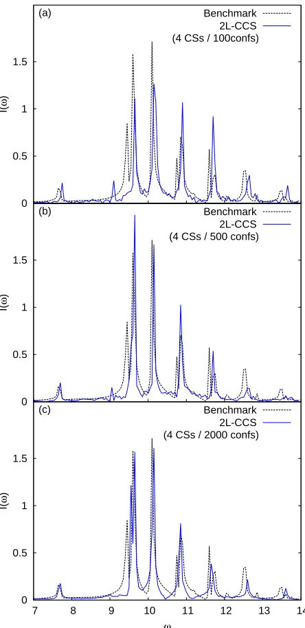
FIG. 5: Comparison of Fourier-transforms from benchmark and 2L-CCS: (a) 1 CS / 2000 confs, (b) 2 CSs / 2000 confs, (c) 4 CSs / 2000 confs
with increasingK.
The quality of short-term propagation also improves with increasing number of configurations, whilst keeping Kfixed, as can be seen in Fig.4. This is illustrated qual-itatively in panels (a)-(c) once more, with the amplitude and phase of the 2LCCS CCF more closely matching that of the benchmark for increasingN, and shown quantita-tively in panel (d) with decreasingχfor increasingN.
Whilst 2L-CCS will be most accurate for short time scales, it is of course worthwhile to check the long time propagation accuracy of the method, accessed via the Fourier-transform of the cross-correlation function after
0 0.5 1 1.5
7 8 9 10 11 12 13 14
I(
ω
)
ω
(4 CSs / 2000 confs)
(c) Benchmark
2L-CCS 0
0.5 1 1.5
I(
ω
)
(b)
(4 CSs / 500 confs) Benchmark 2L-CCS 0
0.5 1 1.5
I(
ω
)
(a)
(4 CSs / 100confs) Benchmark 2L-CCS
FIG. 6: Comparison of Fourier-transforms from benchmark and 2L-CCS: (a) 4 CSs / 100 confs, (b) 4 CSs / 500 confs, (c) 4 CSs / 2000 confs
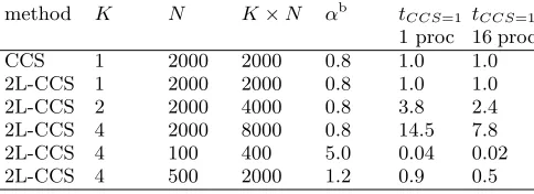
[image:10.612.64.290.58.511.2]method K N K×N αb tCCS=1 tCCS=1
1 proc 16 proc
CCS 1 2000 2000 0.8 1.0 1.0
[image:11.612.54.296.51.139.2]2L-CCS 1 2000 2000 0.8 1.0 1.0 2L-CCS 2 2000 4000 0.8 3.8 2.4 2L-CCS 4 2000 8000 0.8 14.5 7.8 2L-CCS 4 100 400 5.0 0.04 0.02 2L-CCS 4 500 2000 1.2 0.9 0.5
TABLE I: Sampling parameters for the simulations: number of basis vectors per configurationK, number of
configurationsN, compression for the two bath modes αb, execution timetfor one propagation step on 1 and
16 processors, where one CCS step is taken as unity.
improving the treatment of the bath via increasingN is more important for long-term accuracy than improving treatment of the system via increasing K. In Table I it can be seen that by raising the number of configura-tions, the bath compression αb can be reduced until a
stable propagation with good norm-conservation can be obtained. By decompressing the bath modes a greater dynamical region can be covered by the coherent states, precisely the effect that was discussed in Sec. III C.
Despite the fact that increasingN improved the long-term accuracy of this calculation more than increasing K, the fact that increasing both improved the quality of the calculation to some degree demonstrates the ad-ditional layer of flexibility that 2L-CCS presents. This property may be extremely useful for tackling other com-posite problems, especially those where the tunnelling mode may be more complex to represent.
E. Comparison of numerical performance of the 2L-CCS and the standard CCS methods
The time step of integration for both standard CCS and 2L-CCS was ∆t = 0.1 a.u., which gave good norm-conservation for both cases. Numerically the two-layer method scales with the number of basis vectorsKand the number of configurationsN, but its performance – simi-larly to CCS – does not depend explicitly on the number of degrees of freedom. This is due to the fact that neither the CCS Eqs. (13), (15) and (16,17) nor the Ehrenfest-equation (18) scale directly with the dimensionality.
For the standard CCS method withN configurations, an N ×N linear system (16) has to be solved at each time step. For 2L-CCS withK basis vectors per config-uration, (16) has to be solved N times (once per con-figuration) every time step, but the size of each linear system is K ×K. In addition, (19) has to be solved for amplitudeD, which involves a linear system of size N ×N. Solving N linear systems of size K×K and one linear system of size N ×N is more efficient than solving a single [K×N]×[K×N] linear system, as long as K and N are adequately balanced. This means that 2L-CCS will be numerically favourable to a CCS
calcu-lation that has K×N configurations. The comparison of the numerical performance of the two methods can be seen in TableI. The CCS calculation with 2000 configura-tions and the 2L-CCS calculation with 500 configuraconfigura-tions and 4 basis vectors per configuration illustrates the point made above. Although this 2L-CCS calculation is only twice as fast as the CCS calculation on 16 processors, for problems whereK and N can be more evenly balanced (such as real problems with more complicated tunnelling effects) this effect will be significantly enhanced.
The 2L-CCS calculation also benefits from paralleli-sation to a greater extent than CCS, partially demon-strated in TableIand more profoundly shown in Fig. 7. For both CCS and 2L-CCS, as the number of processors increases the bottleneck of the caclulation comes from solution of the system ofN linear equations, Eqs. (16) and (20) respectively. However, in 2L-CCS a propaga-tion step also involves the solupropaga-tion ofN lots of a system ofK linear equations, Eq. (16), which is much quicker. Therefore the rest of the 2L-CCS propagation step can be sped up around the solution of the system ofN linear equations, leading to greater parallel efficiency. It should be noted that this speedup does not take into account basis set generation, as the parallel speedup is based on a propagation step only, however basis set generation is rapid in comparison to propagation. Also, in Fig. 7the speedup of 2L-CCS (1 CS / 2000 conf) is slightly below that of CCS (2000 conf), despite being equivalent calcu-lations. The reason for this is that in 2L-CCS the time dependence of two amplitudes is calculated every prop-agation step (16) and (19), whereas in CCS only one is calculated (16).
The OpenMP shared memory construct was used to parallelise both CCS and 2L-CCS, requiring very little modification of the serial code. This did limit the num-ber of threads to a maximum of 16, as computational hardware with 16 processors was used for the calculations and the general rule of thumb of 1 processor per thread was obeyed. For larger and more complicated calcula-tions MPI parallelisation can be used, although this may require significant restructuring of the serial code. We leave this to further investigations.
IV. CONCLUSIONS
2 4 6 8 10 12 14 16
2 4 6 8 10 12 14 16
Speedup
Number of processors
[image:12.612.57.290.54.223.2]Perfect scaling CCS (2000 confs) 2L-CCS (1 CS / 2000 confs) 2L-CCS (2 CSs / 2000 confs) 2L-CCS (4 CSs / 2000 confs) 2L-CCS (4 CSs / 100 confs) 2L-CCS (4 CSs / 500 confs)
FIG. 7: Parallel speedup for the CCS and 2L-CCS calculations studied in this paper.
fest trajectories. The 2L-CCS method may therefore be seen as a version of MCE where Gaussian CSs are used as a basis for both “quantum” subsystem and “classical” bath.
The scheme was tested on a 20-dimensional asymmet-ric double well potential previously studied by the CCS36, MP/SOFT35and CI expansion37methods. The 2L-CCS method was found to compare favourably with previous results, and with a benchmark study on the potential.38 The scheme was found to converge in both the short and long time scales by increasing the number of “quantum” basis vectors per configuration, K, and the number of configurations,N. Both the short and long term propa-gation represented an improvement over standard CCS, although admittedly it was not significantly closer to the benchmark. However, the purpose of the test with Hamil-tonian (22) was to show the 2L-CCS method works, and converges appropriately. The aim of the scheme is to be implemented in the form of on-the-fly direct dynamics, for which the improved treatment of tunnelling that 2L-CCS offers over 2L-CCS will be extremely beneficial for more challenging real problems.
The 2L-CCS method can also represent an increase in numerical efficiency over the CCS method. For example, a given 2L-CCS calculation which uses K basis vectors andN configurations, will be more numerically efficient than an equivalent CCS calculation which uses K×N configurations. For calculations where K andN can be adequately balanced, this effect will be significant. Fur-thermore, 2L-CCS can benefit greatly from parallelisa-tion, leading to a greater speedup for a propagation step than CCS on the same number of processors.
The application of 2L-CCS to Hamiltonian (22) pro-vided a valid test of an interesting new propagation scheme, and illustrated the flexibility of the wavefunction representation. This can lead to further investigations on composite systems where the quantum and the classical modes can be separated. Furthermore, since the method
is particularly accurate for short-time scales it may be combined with a basis set reprojection technique, allow-ing accurate propagation for a short time period until the basis is required to be re-centered and propagated again for another short time period. Both these advantages of the 2L-CCS method may be utilised for problems such as the modelling of high-order harmonic generation40where the “principal” mode, the motion of an electron which is aligned in the direction of the field, is “quantum” and the other degrees of freedom are “classical”. Investigations are underway.
ACKNOWLEDGEMENTS
Appendix A: Deriving the working equations
In this Appendix the equations for the 2L-CCS method are derived. As mentioned in Sec. II, they do not fol-low from a full variational treatment of the complete wavefunction – where all parameters are optimised at once – but rather from a hierarchical optimisation pro-cedure, where the time-dependent variational principle (TDVP)41is applied to different subsets of parameters at a time. The dynamics of the first layer quantum modes z(q)kn is prescribed according to equations of motion that follow from the TDVP applied to a single CS. In turn, the dynamics of coefficientsaknand classical coordinates z(c)n follows from the TDVP applied to individual
config-urations|φni(and with thez(q)kn regarded as simple
time-dependent functions). The second layer amplitudes Dn
have their dynamics determined from the TDVP applied to the complete wavefunction (with the configurations |φniregarded as a guided basis set).
Let us briefly recall the basic concepts of the TDVP: suppose we are given a trial state |ψi, not necessar-ily normalised, parametrised by a set of n real param-eters (ξ1, ξ2, . . . , ξn)42; this is abbreviated as ψ =ψ(ξ).
The equations of motion for the time-dependent param-eters ξ are obtained by making the action functional S[ψ] = Rt2
t1 Ldt stationary under the boundary
condi-tions: δψ(t1) = δψ∗(t1) = 0 and δψ(t2) =δψ∗(t2) = 0;
here the LagrangianL is
L(ξ,ξ˙) = i 2
hψ|ψ˙i − hψ˙|ψi hψ|ψi −
hψ|Hˆ|ψi
hψ|ψi . (A1) The stationary condition δS = 0 leads directly to the Euler-Lagrange equations:
∂L
∂ξl − d dt
∂L
∂ξ˙l
= 0 for l= 1, . . . , n (A2)
provided all variations δξl can be performed
indepen-dently. From (A2) the equation of motion for each of theξl follows.
The variational solution ψ(t) = ψ(ξ(t)) obtained in this way represents the best achievable solution with the limited set of parametersξ. If there is a sufficient number of parameters (i.e. if the trial state proves to be flexible enough) this solution will converge to the exact solution of the Schr¨odinger equation for the particular system at hand, as long as normalisation is ensured and a proper phase factor, which is just the action S(ψ(t)) = S(ξ(t)) evaluated over the orbit ξ(t), is added to |ψi43. The resulting wavefunction|Ψ(t)irelates to|ψ(t)iin the fol-lowing way:
|Ψ(t)i= p |ψ(t)i
hψ(t)|ψ(t)ie
iS(ψ(t)). (A3)
The overall action phase is immaterial if |Ψ(t)i is to be regarded as the complete wavefunction of the sys-tem in question. However, the fundamental strategy of
the present method is to express the system’s complete wavefunction as a linear combination of such variation-ally optimised solutions, which then act as a guided ba-sis. In this scenario, the phase plays an important role in smoothing out oscillations thus allowing for a more accu-rate description of interference effects between the basis elements.
1. Single CS dynamics
The fundamental block in the standard CCS method and all its variants is the single coherent state: |ψi=|zi. When|zi is used as a trial state in Eq. (A1) we obtain the Lagrangian:
L= i 2(z
∗z˙
−z˙∗z)−Hord(z∗,z) (A4)
where the ordered HamiltonianHord is like in Eq. (12).
Taking z and z∗ as independent variables, the Euler-Lagrange equations (A2) translate to
∂L
∂z∗ − d dt
∂L
∂z˙∗ = 0 (A5)
plus an equivalent complex conjugate equation. The equation of motion forzfollows immediately:
˙
z=−i∂Hord(z ∗,z)
∂z∗ (A6)
which is just the familiar pair of Hamilton equations from classical mechanics, but written in complex notation. The optimised state in this case would be|z(t)ieiS(z(t)).
2. First layer (“quantum” modes)
The prototype system suitable for the method is anM -dimensional system composed of two sub-systems: the first contains a total of M(q) “quantum” DOF and the
second corresponds to the remaining “classical” DOF. The configurations|ϕniin Eq. (8) reads44:
|ϕni= "K
X
k=1
bkn|z(q)kni #
|z(c)mi (A7a)
=
K X
k=1
bkn|zkni (A7b)
where in the second line the primitive CS basis is abbrevi-ated as|zkni=|z(q)kni|z(c)mi. The parameters of each|ϕni
have to be optimised individually, so that later these con-figurations can be used as a guided basis when expressing the complete wavefunction.
coordinates z(q)kn, meanwhile, will have their dynamics prescribed according to the single CS result, Eq. (A6) [which in the present context translates to Eq. (13) of Sec. II]. This is done in order to avoid complicated equa-tions of motion for the coordinatesz(q)kn which would oth-erwise result from the variational procedure.
The first step would be to write down the Lagrangian L of Eq. (A1) taking |ψi = |ϕni. However, owing to
the non-orthogonality of the CSs used in Eq. (A7) this straightforward approach leads to somewhat cumbersome Euler-Lagrange equations.
Aiming at a simpler derivation, we proceed as fol-lows: using a sub-indexnto refer to quantities calculated within then-th configuration, and denoting the norm by
Nn=hϕn|ϕni= K X
kl=1
b∗ knhz
(q)
kn|z
(q)
ln ibln, (A8)
the Lagrangian
Ln= i 2
hϕn|ϕ˙ni − hϕ˙n|ϕni
hϕn|ϕni −
hϕn|Hˆ|ϕni
hϕn|ϕni
(A9)
may be expressed as
Ln= Ln Nn −
i 2
dlogNn
dt (A10)
where the implicitly definedLn, given by
Ln=ihϕn|ϕ˙ni − hϕn|Hˆ|ϕni (A11)
is exactlyLn(Nn= 1).
We wish to work withLn rather than withLn, but we
cannot simply make Nn = 1 in the action functional, as
this prevents us from performing independent variations of the amplitudes bkn, which is a necessary assumption
if the Euler-Lagrange equations are to be obtained. To overcome this, a Lagrange multiplierλn is introduced in
the action functional to take care of the constrainNn= 1;
thus the action can be rewritten as
Sn=S[λn, ϕn] = Z t2
t1
Ln Nn −
λn(Nn−1)
dt (A12)
where the surface terms that come from the derivative −i
2
dlogNn
dt of Eq. (A10) have been omitted for they
van-ish trivially upon variation ofSn.
Let us temporarily denote by{α∗
l, α}the set of
(com-plex) parameters of the trial state: |ϕni =|ϕn(α∗, α)i.
If we impose the conditionδSn = 0 and use the fact that
variations{δλ, δα∗
l, δαl}are now all independent, we find
that the following set of equations must hold:
1 Nn ∂L n ∂α∗ l − d dt ∂Ln ∂α˙∗ l
−
λn+ Ln N2 n ∂N n ∂α∗ l
= 0 (A13a)
1 Nn
∂Ln ∂αl −
d dt
∂Ln ∂α˙l
−
λn+ Ln N2 n ∂Nn ∂αl
= 0 (A13b)
Nn−1 = 0 (A13c)
We shall work with this alternative form of the Euler-Lagrange equations rather than the one in Eq. (A2).
Substituting the configuration ansatz of Eq. (A7), into the LagrangianLn of Eq. (A11), it reads:
Ln=i K X
kl=1
b∗ knhz
(q)
kn|z
(q)
lnib˙ln+b∗knhz
(q)
kn|z˙
(q)
lnibln
+ i 2(z
(c)∗
n z˙(c)n −z˙(nc)∗z(c)n )− hφn|Hˆ|φni. (A14)
Following this, the set of equations (A13) can be rewritten in terms of the different parameters of the trial state: for the classical mode coordinates, we get imme-diately from Eq. (A13a):
∂Ln
∂z(nc)∗
−dtd ∂Ln
∂z˙(nc)∗
= 0 (A15)
sinceNn does not depend upon these coordinates. This
leads at once to the Ehrenfest equation
˙
z(c)n =−i K X
kl=1
b∗
knbklhz(q)kn|z
(q)
lni
∂Hord(z∗kn,zkl) ∂z(nc)∗
, (A16)
which shows that the “classical” modesz(c)n experience a
potential averaged over all sets of quantum modes. On the other hand, for the amplitudesbkn Eqs. (A13)
reduce to
∂Ln ∂bkn −
d dt
∂Ln ∂b˙kn
−(λn+Ln) ∂Nn ∂bkn
= 0 (A17a)
∂Ln ∂b∗
kn
−(λn+Ln) ∂Nn ∂b∗
kn
= 0. (A17b)
These two equations are equivalent but, since ˙b∗
kn does
not appear in Ln, it is easier to work with the second
one. Moreover, becauseNn is linear in the amplitudes,
we can easily find λn by multiplying Eq. (A17b) with b∗
kn, summing over k and using the fact that Nn = 1;
this gives
λn+Ln= K X k=1 b∗ kn ∂Ln ∂b∗ kn
,≡υ˙n (A18)
where the quantity ˙υn is defined for convenience. Hence,
combining Eqs. (A18) and (A17b), it follows that
K X
l=1
hz(q)kn|z(q)lni(ib˙ln−υ˙nbln)
=
K X
l=1
hz(q)kn|z(q)lni
"
H(z∗kn,zln)−ih
z(q)kn|z˙(q)ln i hz(q)kn|z(q)ln i
#
bln.
(A19)
Finally, we introduce new amplitudes dnk according to
the following transformation:
bkn= (dkneiS (q)
kn)e−iυn= (akne−iθ
(c)
whereaknare identified as the coefficients in (8) andS
(q)
kn
is the quantity
Skn(q)=
Z t
0
i
2(z
(q)∗ kn z˙
(q)
kn −z˙
(q)∗
kn z
(q)
kn)−Hord(z∗kn,zkn)
dt′
(A21) which can be interpreted as the action of the quantum modes with the classical subsystem regarded as an exter-nal system.
The purpose of the change of variables in Eq. (A20) is threefold: first, it effectively cancels the ˙υn on the
left-hand side of Eq. (A 2); second, the derivative of the action ˙Sln(q), when combined with the remaining terms on the right-hand side of Eq. (A 2), gives the familiar CCS equation for the new amplitudesdkn – which is exactly
Eqs. (16-17) of Sec. II– and third: if the configuration |ϕni is rewritten together with its phase S(ϕn) [as it
appears in the full wavefunction ansatz; see Eq. (A23) below] in terms of the new amplitudes dkn, we recover
the optimised phase for the quantum basis functions:
|ϕnieiS(ϕn)= " K
X
k=1
dkn|z(q)knieiS (q)
kn
#
|z(c)n ieiθ(c)m (A22a)
=
K X
k=1
dkn|zknieiSkn , (A22b)
where in the last equationSknis the action defined in Eq.
(15) of Sec. II. Notice that when we write the configura-tion as in (A22a), explicitly separating the subsystems, we see that the “classical” modes |z(c)n i are left with a
geometric phaseθ(c)n =2i Rt
0(z (c)∗
n z˙(c)n −z˙n(c)∗z(c)n )dt′.
3. Second layer (“classical” modes)
As stated earlier, the basic idea in the two-layer formu-lation is to use the optimised configurations of Eq. (A22) as the basis functions for the complete wavefunction of the system|Φiwhich is
|Φi=
N X
n=1
An|ϕnieiS(ϕn). (A23)
We shall once again employ the TDVP, this time taking only the amplitudesAn as variational parameters, while
using the previously individually optimised dynamics for the configurations|ϕni; the implicit assumption is that
the single-configuration dynamics can be regarded as a good approximation for the dynamics that would result from a full variational approach.
As in the previous case, it is convenient to work with the LagrangianL, defined as:
L=ihΦ|Φ˙i − hΦ|Hˆ|Φi (A24)
and the alternative action functional in Eq. (A12), which includes a Lagrange multiplier to enforce normalisation. Here, the normN reads:
N=hΦ|Φi=
N X
mn=1
A∗
nAmhϕn|ϕmiei(S(ϕm)−S(ϕn)),
(A25) whileLis explicitly given by the expression:
L=
N X
nm=1
h
iA∗
nA˙mhϕn|ϕmi
+A∗ nAm
ihϕn|ϕ˙mi −S˙ϕmhϕn|ϕmi
−A∗
nAmhϕn|Hˆ|ϕmi i
ei(S(ϕm)−S(ϕn)). (A26)
The formalism developed earlier applies here in the exact same manner; in the present context, the Euler-Lagrange equation (A13b) translates to
∂L ∂A∗ n
−(λ+L)∂N ∂A∗ n
= 0 (A27)
sinceLof Eq. (A26) does not depend on ˙A∗
n. The value
of the multiplier can be obtained as before; this time, sinceA∗
n appears linearly in all the terms ofL, we find
λ=
N X
n=1
A∗ n
∂L ∂A∗
n
so that the equation forA reads:
N X
m=1
hϕn|ϕmi(iA˙m−LAm)ei(S(ϕm)−S(ϕn))
=
N X
m=1
h
hϕn|Hˆ|ϕmi −ihϕn|ϕ˙mi
+ ˙Smhϕn|ϕmi i
Amei(S(ϕm)−S(ϕn)). (A29)
Defining new amplitudesDmthrough the relation
Am=Dme−iS (A30)
we are directly led to Eq. (19) of Sec. II, from where the equations of motion (20-21) forDn follows.
Finally, we write down the phase-corrected complete wavefunction|Ψi=|ΦieiS:
|Ψi=
N X
n=1
Dn|ϕnieiS(ϕn) (A31a)
=
N X
n=1
Dn " K
X
k=1
dkn|z
(q)
knie iS(q)kn
#
|z(c)n ieiθm(c) (A31b)
=
N X
n=1
Dn K X
k=1
dkn|zknieiSkn (A31c)
which is exactly Eq. (9c) given in Section II [after sub-stituting akn for dkn in that equation, using Eq. (14)].
This completes the derivation of the working equations of the 2L-CCS method.
Appendix B: Benchmark calculations
The wavefunction is represented as a basis set expan-sion
|Ψ(t)i=
Nbth X
j=1
Nsys X
n=1
cjn(t)|ψjbi|ψnsi, (B1)
in whichcjn(t) are complex, time-dependent amplitudes,
|ψb
ji is a time-independent basis function for the bath
modes and|ψs
niis a time-independent basis function for
the system mode. The number of bath and system basis functions are given byNbth and Nsys respectively.
Sub-stitution into the time-dependent Schr¨odinger equation leads to an equation for the time-dependence of the am-plitudes
dcim(t)
dt =−i Nbth
X
j=1
Nsys X
n=1
Himjncjn(t), (B2)
whereHimjn is the Hamiltonian matrix
Himjn=hψibψsm|Hˆ|ψbjψnsi
=hψms|pˆ (1)2
2 −
ˆ q(1)2
2 +
ˆ q(1)4
16η|ψ
s
niδij
+hψib|Pˆ 2
2 + ˆ Q2
2 |ψ
b
jiδmn
+λ 2hψ
b
i|Qˆ2|ψjbihψms |qˆ(1)|ψnsi.
(B3)
The bath and system basis functions are orthonormal (see below), a fact that has been exploited in the above. The bath modes are nearly harmonic, therefore they can be represented by harmonic oscillator basis functions. A complete description of the bath would involve all ex-cited state configurations, however in practice we can simply add on configurations until a converged result is achieved. For an M −1 dimensional bath, an excited state is comprised of the product ofM−1 single particle harmonic oscillator functions,QM
l=2|χ(l)i, with different
benchmark result for Hamiltonian (22), then the bath basis functions are:
|ψ1bi= |0000. . .0000i
|ψ2bi= (|2000. . .0000i+· · ·+|0000. . .0002i) ×1/√M −1
|ψ3bi= (|4000. . .0000i+· · ·+|0000. . .0004i) ×1/√M −1
|ψ4bi= (|2200. . .0000i+· · ·+|0000. . .0022i) ×√2!/p(M −1)(M−2)
|ψb
5i= (|6000. . .0000i+· · ·+|0000. . .0006i) ×1/√M −1
|ψ6bi= (|4200. . .0000i+· · ·+|0000. . .0024i) ×1/p(M −1)(M−2)
|ψb
7i= (|2220. . .0000i+· · ·+|0000. . .0222i) ×√3!/p(M −1)(M−2)(M −3) |ψ8bi= (|8000. . .0000i+· · ·+|0000. . .0008i)
×1/√M −1 |ψb
9i= (|6200. . .0000i+· · ·+|0000. . .0026i) ×1/p(M −1)(M−2)
|ψ10bi= (|4400. . .0000i+· · ·+|0000. . .0044i) ×√2!/p(M −1)(M−2)
|ψ11bi= (|4220. . .0000i+· · ·+|0000. . .0224i) ×√2!/p(M −1)(M−2)(M −3) |ψ12bi= (|2222. . .0000i+· · ·+|0000. . .2222i)
×√4!/p(M −1)(M−2)(M −3)(M−4) (B4)
with relevant normalisation factors included. The square of the normalisation factors is simply equal to the number of configurations grouped; in this case there are 8855 bath configurations governed by only 12 distinct amplitudes.
The basis functions for the system are those of a rect-angular box
hq(1)|ψsni= r
2 Lsin
nπ
L (q
(1)
−qbox)
, (B5)
with L being the size of the box and qbox its left hand
coordinate. Values of L = 12 and qbox = −6 are used
to enable a large enough area of coordiante space to be covered.
Now the basis functions have been defined, the matrix elements of the Hamiltonian may be evaluated. Firstly,
the bath elements
hψib| ˆ P2
2 + ˆ Q2
2 |ψ
b
ji=δij
Ei+
M−1
2
(B6)
are simply the harmonic oscillator eigenvalues for the ex-cited states. The value ofEi is the sum of quanta in a
particular excited stateEi =PMl=2ǫ (l)
i , where ǫ
(l)
i is the
number of quanta in one mode. Secondly, the system elements
hψsm|pˆ (1)2
2 −
ˆ q(1)2
2 +
ˆ q(1)4
16η |ψ
s
ni=
n2π2
2L2 δmn +
2 L
qbox+L Z
qbox
sinmπ L (q
(1)
−qbox)
×sinnπ L (q
(1)−q box)
qˆ(1) 4
16η − ˆ q(1)2
2
!
dq(1),
(B7)
are the particle in a box energy levels, plus an additional potential term. Finally, the system-bath interaction ele-ments are given as
hψib|Qˆ2|ψbji=
= Aij 2 q
(ǫ(il)+ 2)(ǫ(il)+ 1) ifǫ(il)=ǫ(jl)−2 in only one mode and ǫ(il)=ǫ(jl)
in all other modes Aij
2
q
ǫ(il)(ǫ(il)−1) ifǫ(il)=ǫ(jl)+ 2 in only one mode and ǫ(il)=ǫ(jl)
in all other modes
M X
l=2
ǫ(il)+M−1
2 ifǫ
(l)
i =ǫ
(l)
j
in all modes
0 if states differ by more
than two quanta in one mode, or two quanta in more than one mode
(B8)
hψsm|qˆ(1)|ψsni=
2 L
qbox+L Z
qbox
sinmπ L (q
(1)
−qbox)
×sinnπ L (q
(1)−q box)
q(1)dq(1),
(B9)
whereAijis a constant that depends upon the
normalisa-tion factors and the number of configuranormalisa-tions that differ by only two quanta in one mode between states. For clar-ity, thehψb
i|Qˆ2|ψbjimatrix elements evaluated using the
|ψb
1i |ψb2i |ψb3i |ψ4bi |ψ5bi |ψb6i |ψ7bi |ψ8bi |ψ9bi |ψb10i |ψb11i |ψb12i hψb
1| M2−1 √2(
M−1)
2 0 0 0 0 0 0 0 0 0 0
hψb 2|
√ 2(M−1)
2 2 +
M−1 2
√
3 √M−2 0 0 0 0 0 0 0 0
hψb 3| 0
√
3 4 +M−1
2 0 12
√ 30
√ 2(M−2)
2 0 0 0 0 0 0
hψb 4| 0
√
M−2 0 4 +M−1
2 0
√ 6
√6(
M−3)
2 0 0 0 0 0
hψb
5| 0 0 12
√
30 0 6 +M−1
2 0 0
1 2 √
56
√2(M−2)
2 0 0 0
hψb
6| 0 0
√ 2(M−2)
2
√
6 0 6 +M−1
2 0 0
1 2 √ 30 1 2 √
24 √M−3 0
hψb
7| 0 0 0
√ 6(M−3)
2 0 0 6 +M2−1 0 0 0 12
√ 36 p
2(M−4) hψb
8| 0 0 0 0 12
√
56 0 0 8 +M−1
2 0 0 0 0
hψb
9| 0 0 0 0
√2(
M−2) 2
1 2 √
30 0 0 8 +M−1
2 0 0 0
hψb
10| 0 0 0 0 0 12
√
24 0 0 0 8 +M−1
2 0 0
hψb
11| 0 0 0 0 0
√
M−3 1
2 √
36 0 0 0 8 +M−1
2 0
hψb
12| 0 0 0 0 0 0
p
2(M−4) 0 0 0 0 8 +M−1
2 (B10)
The initial amplitudes are calculated via projection onto the initial wavepacket, with all modes in the ground vi-brational level att= 0
cim(0) =hψbiψms |Ψ(0)i=δ1mhψsm|Ψ(0)i
=
r
2 L
qbox+L Z
qbox
sinmπ L (q
(1)
−qbox)
× 1 π 14 exp −1 2
q(1)−q(1)(0)2
dq(1).
(B11)
The CCF is calculated via the overlap between the wave-function and the mirror image of the initial state,
CCF(t) =hΨ(0)¯ |Ψ(t)i
= Nbth X i,j=1 Nsys X m,n=1 ¯ c∗
im(0)cjn(t)hψibψsm|ψjbψsni
= Nbth X i,j=1 Nsys X m,n=1 ¯ c∗
im(0)cjn(t)δijδmn
= Nbth X j=1 Nsys X n=1 ¯ c∗
jn(0)cjn(t).
(B12)
where the mirror image of the initial state has been ex-pressed as the basis set expansion with coefficients ¯cjn,
and the orthogonality of the basis functions has been utilised.
The benchmark is converged with respect toNbth and
Nsys, with fully converged values ofNbth= 12 (number
of basis functions to give even harmonic oscillator excited states up to a quanta of 8) andNsys= 50.
REFERENCES
1H.-D. Meyer, U. Manthe, and L. S. Cederbaum,Chem. Phys.
Lett.165, 73 (1990).
2C. Lubich,From Quantum to Classical Molecular Dynamics: Re-duced Models and Numerical Analysis, Zurich Lectures in Ad-vanced Mathematics (European Mathematical Society (EMS), 2008).
3H. Wang and M. Thoss,J. Chem. Phys.119, 1289 (2003). 4U. Manthe,J. Chem. Phys.128, 22 (2008).
5O. Vendrell and H.-D. Meyer,J. Chem. Phys.134, 044135 (2011). 6S. R¨omer, M. Ruckenbauer, and I. Burghardt,J. Chem. Phys.
138, 064106 (2013).
7E. J. Heller,J. Chem. Phys.75, 2923 (1981).
8D. V. Shalashilin and M. S. Child,J. Chem. Phys.113, 10028
(2000).
9M. F. Herman and E. Kluk,Chem. Phys.91, 27 (1984). 10E. Kluk, M. F. Herman, and H. L. Davis, J. Chem. Phys.84,
326 (1986).
11K. G. Kay,Chem. Phys.322, 3 (2006).
12T. J. Martinez, M. Ben-Nun, and G. Ashkenazi,J. Chem. Phys. 104, 2847 (1996).
13M. Ben-Nun and T. J. Mart´ınez,Adv. in Chem. Phys.121, 439
(2002).
14D. V. Shalashilin and M. S. Child, J. Chem. Phys. 115, 5367
(2001).
15D. V. Shalashilin and M. S. Child,Chem. Phys.304, 103 (2004). 16D. V. Shalashilin and M. S. Child,J. Chem. Phys.128, 054102
(2008).
17G. A. Worth and I. Burghardt, Chem. Phys. Lett. 368, 502
(2003).
18D. V. Shalashilin and I. Burghardt,J. Chem. Phys.129, 084104
(2008).
19D. V. Shalashilin,J. Chem. Phys.130, 244101 (2009). 20D. V. Shalashilin,J. Chem. Phys.132, 244111 (2010). 21D. V. Shalashilin,Faraday Discuss.153, 105 (2011).
22S.-Y. Ye, D. Shalashilin, and A. Serafini, Phys. Rev. A 86,
032312 (2012).
23I. Burghardt, H.-D. Meyer, and L. S. Cederbaum, J. Chem.
Phys.111, 2927 (1999).
24S. K. Reed, M. L. Gonz´alez-Mart´ınez, J. Rubayo-Soneira, and D. V. Shalashilin,J. Chem. Phys.134, 054110 (2011).
25K. Saita and D. V. Shalashilin, J. Chem. Phys.137, 22A506
(2012).
26K. Saita, M. G. D. Nix, and D. V. Shalashilin, Phys. Chem.
Chem. Phys.15, 16227 (2013).
27D. V. Makhov, W. J. Glover, T. J. Martinez, and D. V. Sha-lashilin,J. Chem. Phys.141, 054110 (2014).
28D. V. Makhov, K. Saita, T. J. Martinez, and D. V. Shalashilin,
29G. D. Billing,J. Chem. Phys.65, 1 (1976). 30G. D. Billing,Chem. Phys. Lett.100, 535 (1983).
31G. D. Billing,The Quantum Classical Theory(Oxford University Press, Oxford, NY, 2003).
32J. R. Klauder and B. S. Skagerstam,Coherent States: Appli-cations in Physics and Mathematical Physics(World Scientific, Singapore, 1985).
33S. R¨omer and I. Burghardt,Mol. Phys.111, 3618 (2013). 34M. Ronto and D. V. Shalashilin,J. Phys. Chem. A 117, 6948
(2013).
35Y. Wu and V. S. Batista,J. Chem. Phys.121, 1676 (2004). 36P. A. Sherratt, D. V. Shalashillin, and M. S. Child,Chem. Phys.
322, 127 (2006).
37S. Habershon,J. Chem. Phys.136, 054109 (2012).
38J. A. Green and D. V. Shalashilin,Chem. Phys. Lett.641, 173
(2015).
39D. V. Shalashilin, M. S. Child, and D. C. Clary,J. Chem. Phys. 120, 5608 (2004).
40C. Symonds, J. Wu, M. Ronto, C. Zagoya, C. Figueira de Moris-son Faria, and D. V. Shalashilin,Phys. Rev. A91, 023427 (2015). 41P. Kramer and M. Saraceno,Geometry of the Time-Dependent Variational Principle in Quantum Mechanics, Lecture Notes in Physics, Vol. 140 (Springer, Berlin, Heidelberg, 1981).
42We assume real parameters for simplicity, but, of course, this also accounts for complex parametrisations: one can always work sep-arately with real and imaginary parts or, alternatively, treat the parameters and their complex conjugates as independent vari-ables – both approaches are equivalent.
43In order to come to this conclusion one must consider the case of unrestricted variations and work out the Euler-Lagrange equations of motion; the resulting equation coincides with the Schr¨odinger equation except for a time-dependent phase; both normalisation factor and action phase are introduced precisely to cancel this factor.