This is a repository copy of Redistricting decisions for local government rationalization: Models and applications.
White Rose Research Online URL for this paper: http://eprints.whiterose.ac.uk/105181/
Version: Accepted Version
Article:
Bruno, G., Genovese, A. orcid.org/0000-0002-5652-4634 and Piccolo, C. (2016) Redistricting decisions for local government rationalization: Models and applications. Socio-Economic Planning Sciences. ISSN 1873-6041
https://doi.org/10.1016/j.seps.2016.09.006
eprints@whiterose.ac.uk https://eprints.whiterose.ac.uk/
Reuse
This article is distributed under the terms of the Creative Commons Attribution-NonCommercial-NoDerivs (CC BY-NC-ND) licence. This licence only allows you to download this work and share it with others as long as you credit the authors, but you can’t change the article in any way or use it commercially. More
information and the full terms of the licence here: https://creativecommons.org/licenses/
Takedown
If you consider content in White Rose Research Online to be in breach of UK law, please notify us by
Territorial Amalgamation Decisions in Local Government: Models and a Case Study from Italy
Giuseppe Bruno1, Andrea Genovese2, Carmela Piccolo1
1 Department of Industrial Engineering, University of Naples Federico II,
Piazzale Tecchio, 80 – 80125 Naples, Italy giuseppe.bruno@unina.it, carmela.piccolo@unina.it
2 Management School, University of Sheffield,
Conduit Road, S10 1FL, Sheffield, UK a.genovese@shef.ac.uk
Abstract
In the context of general welfare reforms in western economies, a recent trend has concerned the rationalization of administrative structures of local authorities, including a reduction in the number of administrative levels and units (through mergers and amalgamation processes) and the subsequent rearrangement of their boundaries. In this paper, we develop mathematical models to analyze amalgamation and redistricting policy decisions implemented in Italy. Results provided by such models can provide valuable support to stakeholders and policy makers.
1. Introduction
difficulty of combining the need for more efficient territorial configurations and the safeguard of public services accessibility in local communities.
As stated by Meligrana (2005) and Allers and Geertsema (2016), while local government organization is under significant pressure for reform, there is a historical lack of methods and tools that could help officials in making these decisions. As an effect, such decisions are often performed by using ad-hoc procedures.
In this work, the problem of reorganizing Italian administrative subdivisions has been formulated in terms of a redistricting problem. In such a problem, an initial district map is already available; more precisely, territorial units (municipalities and/or local communities) of a given region are already grouped in districts (provinces). Within each district, a local authority is responsible for providing many essential services through some facilities (generally located in the chief-town). Specifically, Italian provinces provide the following services to the local populations: highways design, maintenance and upgrades; education planning (staff and resource planning, provision of vocational qualification courses, design, maintenance and upgrades of school facilities); public transport provision; environmental protection (waste, water and energy management and planning, disaster relief services); welfare and social security. Since the aim is to reduce the number of active districts, resulting new local authorities will need to serve wider areas, with some potential effects on the population that should be carefully assessed.
Considering this specific problem, some novel mathematical programming formulations (adaptable to analyze similar problems in different contexts) will be proposed in this paper; also, results provided by these models will be compared to the amalgamation proposals by the Italian government.
The remainder of the paper is organized as follows: the next section is devoted to the description of the Italian administrative system and of the current subdivision of the territory in provinces. Then, an overview of the literature background is provided; subsequently, some mathematical models are introduced to address the specific Italian redistricting problem. Results provided by the application of the different models to a real case study are analyzed and compared. Finally, conclusions are drawn, along with future research directions.
2. The Italian provinces
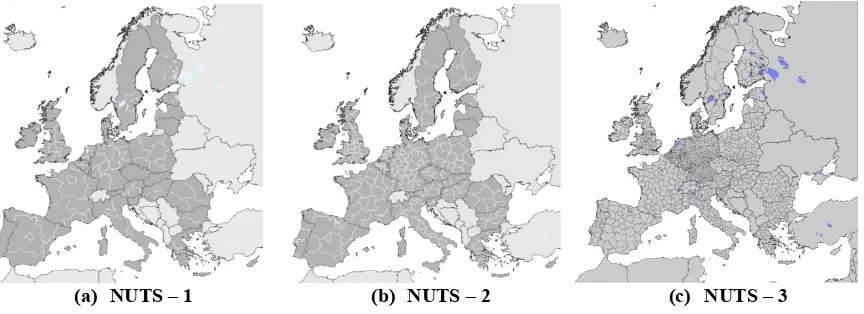
countries. However, if compared with more similar countries, Italian provinces (NUTS 3) are the smaller and less populated ones.
(a) NUTS – 1 (b) NUTS – 2 (c) NUTS – 3
Figure 1 – Subdivision of UE countries according to EUROSTAT (2002) Nomenclature of Units for Territorial Statistics (NUTS)
COUNTRY NUTS 1 NUTS 2 NUTS 3
Inhabitants (A)
Area
(B) # (A1) (B1) # (A2) (B2) # (A3) (B3)
France 65.447.374 543.965 9 7.271.930 60.440 26 2.517.207 20.921 100 654.474 5.439
Germany 83.000.000 357.023 16 5.187.500 22.313 39 2.128.205 9.154 429 193.473 832
Italy 60.626.442 301.340 5 12.125.288 60.268 21 2.886.973 14.349 110 551.149 2.739
Poland 38.626.349 313.893 6 6.437.725 52.315 16 2.414.147 19.618 66 585.248 4.755
Spain 43.967.766 504.614 7 6.281.109 72.087 19 2.314.093 26.558 59 745.216 8.552
[image:4.595.88.520.119.276.2]UK 63.181.775 244.820 9 7.020.197 27.202 30 2.106.059 8.160 93 679.374 2.632
Table 1 – Number and size of NUTS 1,2,3 in the main EU countries
Due to the general political and economic context, the current partition of the Italian territory in provinces is considered unsustainable. Hence, the central government has promoted several reform projects aimed at reducing the number of provinces. After several consultations, the implementation of such projects has been articulated in two subsequent steps: (i) the identification of provinces to be suppressed; (ii) the re-aggregation, at a regional level, of suppressed provinces to the remaining ones.
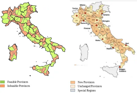
The first step was performed through the definition of some feasibility requirements
(Gazzetta Ufficiale, 2012); in particular, it was established that provinces with an area lower than 2500 km2 or a population of less than 350,000 inhabitants should have been deactivated.
Feasible Provinces Infeasible Provinces
New Provinces Unchanged Provinces Special Regions
Figure 2 – Feasible and Infeasible provinces Figure 3 – Government Proposal
3. Literature background
The debate about the optimal configuration of local government, in terms of administrative levels and size of jurisdictions is not new. Oates’ (1972) decentralization theorem suggests that smaller administrative districts could provide a better solution for accommodating local needs of cost-effective provision of public services (especially in heterogeneous territorial contexts). However, recent cuts to public expenditure impose the design of jurisdictions that are sufficiently large, by implementing amalgamation processes (often promoted through top-down reform processes). Starting from a reduction in the number of Local Authorities (obtained through merging and boundary alteration processes), these processes seek to rationalize systems providing public services (such as healthcare, education, public administration and justice at a territorial level), with the ultimate aim of taking advantage of economies of size (Allers and Geertsema, 2016).
Amalgamation decisions generally involve an element of territorial design; existing jurisdictions should be merged or undergo a process of boundary alteration in order to create a new territorial design meeting certain conditions.
In the extant literature, the process of creating regions, starting from elementary units is referred to by wide range of names, including region-building (Byfuglien and Nordgard, 1973), regional clustering (Maravalle and Simeone, 1995), regionalization (Wise et al., 1997), territorial districting, with the latter being, by far, the most prolific literature stream, as testified by surveys appeared in the last decades (Duque et al., 2007; Kalcsics, 2015).
[image:5.595.73.519.70.374.2]units, each of them associated with a set of attributes (e.g., population, area), that have to be grouped in districts in such a way that constraints on their dimension and topology are satisfied. Constraints on the dimensions typically involve limitations on maximum and/or minimum population and/or area to be assigned to each district. Topological properties may involve the contiguity of districts (i.e., districts should not be divided into two or more geographically separate entities) and their compactness (i.e., the extent to which the shape of a district is spread out from its center and the regularity of its boundaries). Other conditions may include the respect of natural borders or of pre-existing administrative partitions, as well as aspects concerned with socio-economical homogeneity. Territorial districting problems are suitable to describe a wide variety of decision-making issues; hence, a variety of models and algorithms have been proposed in order to deal with applications in the fields of public and private services. In this case, the goal is to design sub-areas for which facilities are responsible for service provision. In this context, many authors dealt with the problem of the school districting, i.e., the problem of identifying the groups of children attending each school (see e.g. Ferland and Guénette, 1990; Schoepfle and Church, 1991); others addressed the problem of organizing the solid waste disposal service, i.e. the partitioning of the streets in which waste need to be collected into sectors that have to be visited by single garbage trucks (Hanafi et al.,1999). In these cases, contiguity and compactness properties are utilized as a proxy for the accessibility of the services provided at district centers.
Another application is related to the design of political districts, i.e., electoral constituencies. In such context, the goal is to partition the territory under consideration in such a way that no political party should be able to take advantage from the territorial subdivision (see e.g. Hess et al., 1965; Williams, 1995; Hojati, 1996; George et al., 1997; Mehrotra et al., 1998; Bozkaya et al., 2003, Ricca and Simeone, 2008; Ricca et al., 2011). In this specific case, constraints about contiguity and compactness have the main aim of ensuring that resulting districts will have regular shapes, as a way to guarantee the impartiality of the map.
Within the political districting body of literature, significant attention has been devoted to
redistricting problems. Indeed, due to demographic changes, the partition of an area into electoral districts must be constantly reviewed and modified (Williams, 1995, Kalcsics, 2015). As such, redistricting approaches are mainly concerned with the use of local search techniques and/or metaheuristics in the design of an improved district map, by gradually modifying the initial one, for example by swapping units between neighboring districts (Browdy, 1990; D’Amico et al., 2002; Bozkaya et al., 2003).
In this work, we want to address a similar problem in which an amalgamation process of local authorities needs to be conducted, due to economic reasons that impose to reduce the number of facilities providing services and, hence, active districts. In such process, the damage on the population in terms of accessibility to the services must be minimized. Coherently to discussed service-oriented territorial districting problems, contiguity and compactness properties will be utilized as a proxy for district centers accessibility.
The following section will propose some mathematical models to deal with the described problem.
4. Optimization models for the reorder of the Italian provinces
In the current Italian local government structure, each region is composed of a certain number of municipalities grouped in provinces. Moreover, within each province, a specific municipality (named chief town) hosts facilities providing a set of services to the local population. In order to reduce the total management costs, the Italian central government promoted a reorganization of the current administrative structure, by reducing the number of provinces, and, therefore, chief towns. In order to guide such process, some requirements were defined (Corriere della Sera, 2013), in terms of minimum population (300000 inhabitants) and area (2500 km2) of the provinces. In the following, we will indicate as:
- Feasible, a district meeting the defined requirements; - Infeasible, a district not meeting the defined requirements.
The proposed models will have to deal with two different type of decisions:
closure decisions, i.e. the identification of the subset of chief towns to be closed;
reallocation decisions, i.e. the reassignment of territorial units to active chief towns. Closure decisions will be strongly influenced by the definition of governmental requirements. However, two different approaches were formulated in order to take such requirements into account in the models:
a prescriptive approach, for which all districts not meeting the requirements in the current configuration have to be closed (this is the one adopted by the Italian government in the formulation of its proposal);
an optimal approach, for which the model may decide the administrative chief towns to be closed, provided that in the final configuration all districts meet the given requirements.
In practice, the number of districts in the solution provided by the prescriptive approach is given a priori, by the number of feasible districts.
Similarly, also for the reallocation decisions, two different strategies were defined:
Merging existing districts, i.e. reallocating entire closed districts to one of the active chief towns (this is the approach adopted by the Italian government in the formulation of its proposal);
Reassigning territorial units, i.e. performing a reallocation process of single municipalities to active chief towns.
number of active districts, as discussed in Andrews and Boyne (2012) and Allers and Geertsema (2016).
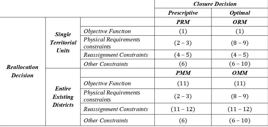
By combining these approaches, four classes of redistricting models can be introduced (Table 2). Closure Decision Prescriptive Optimal Single Territorial Units Prescriptive Reassigning Model (PRM) Optimal Reassigning Model (ORM) Reallocation Decision Entire Existing Districts Prescriptive Merging Model (PMM) Optimal Merging Model (OMM)
Table 2 – Classes of redistricting problems
Despite the specific adopted approach, a common structure can be traced in the four models, composed by the following main components:
objective function, defined in terms of compactness of the resulting districts. Such objective, usually employed in the districting models, is particularly appropriate as it represents a proxy of users’ accessibility;
constraints on physical requirements, in order to take into account the conditions imposed by the decision-maker (for instance, constraints on the minimum and maximum districts’ size);
reassignment constraints, to rule the reassignment of territorial units to active districts and chief towns;
other constraints, including further aspects of the problem, such as the contiguity of resulting districts, the respect of pre-existing boundaries, the presence of special districts.
Moreover, a common notation can be introduced:
index associated with the generic territorial unit ( );
� � ∈ �= {1…�}
index associated with the generic existing district ( );
� � ∈ �= {1…�}
set of special districts ( );
�∗ ⊂ �
|
�∗|
=�chief town of district j, i.e. unit in which the facility providing services
��∈ �
is located;
centroid of district j, corresponding to the solution of a weighted
��∈ � 1‒
median problem within the district j;
binary label equal to 1 if unit is initially allocated to district , 0
��� � �
otherwise;
distance between units and .
Furthermore, the following sets of decision variables have to be defined:
binary variable equal to 1 if and only if the chief town of district gets
�� �
closed;
binary variable equal to 1 if and only if unit i is assigned to the chief
���
town of district .�
Formulations are presented assuming that requirements are defined in terms of minimum population and area per each district; therefore, the further notation below has to be considered:
population of unit ;
�� �
area of unit ;
�� �
total population of district ;
��=∑� ∈ ������ �
total area of district ;
��=∑� ∈ ������ �
minimum required population per district;
����
minimum required area per district.
����
In the following, the mathematical formulations of the proposed models are introduced. In particular, for the sake of clarity, we opted for introducing first the class of Reassigning models and then the Merging ones, describing within each class the Prescriptive and the Optimal approaches. In fact, the merging strategy may be viewed as a particular case of the reassigning strategy and, hence, the related models may be formulated by properly adapting reassigning models.
4.1 Reassigning Models (Prescriptive vs Optimal)
The Prescriptive Reassigning Model (PRM) considers the shut-down of chief towns that do not meet the requirement and the subsequent reassignment of the related territorial units (previously part of this suppressed district) to the ones that have been kept active. The PRM
can be formulated as follows:
min�=
∑
� ∈ �∑
� ∈ ����2
������ (1)
����(1‒ ��)≤ �� ∀� ∈ � ‒ �∗ (2)
����(1‒ ��)≤ �� ∀� ∈ � ‒ �∗ (3)
(
1‒ ��)
���≤ ���≤1‒ �� ∀� ∈ �,∀� ∈ � (4)∑
� ∈ ����= 1 ∀� ∈ � (5)��= 0 ∀� ∈ �∗ (6)
The objective function (1) is one of the classical measures of compactness, defined as the weighted sum of the square of the distances among each unit and the chief town of its � assigned district .�
Constraints (2-3) represent governmental requirements. In particular, they impose that only districts having an area larger than ���� and a population larger than���� can be kept open.
Expressions (4-5) deal with reassignment constraints, which rule the reallocation mechanism of territorial units to districts that have been kept active. In particular, constraints (4) impose that only units belonging to closed districts can be affected by reallocation decisions, being redistributed across active districts, while constraints (5) ensure the allocation of each territorial unit to one (and only one) district. Equations (6) represent an example of additional constraints, indicating the presence of a set of special districts that cannot be closed. Finally, constraints (7) define the nature of the decision variables being introduced in the model.
The Optimal Reassigning Model (ORM) differs from the PRM for the criterion used to select districts to be closed. In this case, every district, apart from the special ones, represents a candidate for the closure. Then, the model is aimed at determining how many and which chief towns have to be closed, in such a way that the reassignment process will produce new feasible districts. Among all the solutions, the model selects the most efficient one in terms of objective function, minimizing the average distance between each territorial unit and its own chief town (1). In this case, in the formulation, it is sufficient to replace the groups of constraints (2-3) with the following ones:
∑
� ∈ ������≥ ����(1‒ ��) ∀� ∈ � ‒ �∗ (8)∑
� ∈ ������≥ ����(1‒ ��) ∀� ∈ � ‒ �∗ (9)Constraints (8) assure that the population of a district which is kept active
(
��= 0)
is at leastequal to ����, while constraints (9) impose similar conditions on the area.
The ORM identifies the minimum number �∗ of chief towns to be closed in order to produce feasible districts. However, it is also possible to include in the model an additional constraint about the desired number of chief-towns to be closed:�
∑
� ∈ �
��=� (10)
Of course, in order to find feasible solutions, must be larger or equal than � �∗.
Both the versions of the model may also include an explicit formulation of the contiguity condition.
4.2 Merging Models (Prescriptive vs Optimal)
In this class of models, the strategy consists of aggregating entire existing districts. With this aim, each current district � can be considered as a single territorial unit (�=�), with the total population �� and area concentrated in correspondence of its �� centroid��. Then, here, the
current configuration, each centroid ��is assigned to the related chief town ; therefore, ��
{
���}
is an identity matrix of order . When a certain � ��gets closed, the related district, as a whole,
has to be assigned to another active chief town and, hence, to be merged with another district. In particular, the Prescriptive Merging Model (PMM) closes the chief towns that do not meet the requirements (2-3) and reassigns the related entire districts to the ones that have been kept active.
On the other hand, the Optimal Merging Model (OMM) determines the chief town to be closed in such a way that the reassignment of the related districts will produce new feasible districts.
Compared with the mathematical formulations of the PRM and ORM, the corresponding merging models require the following modifications:
the objective function (1) has to be modified in order to consider the distance between the centroid of each district � ∈ � and its assigned chief town, weighted by the total population of the district itself:
�=∑�,� ∈ ��������2 ��� (11)
the reassignment constraints (4-5) have to be adapted by considering that each district represents a single territorial unit (�=�):
(
1‒ ��)
���≤ ���≤1‒ �� ∀�,� ∈ � (12)∑
� ∈ ����= 1 ∀� ∈ � (13)
[image:11.595.80.516.483.690.2]Also in this case, both the versions of the model may include an explicit formulation of the contiguity condition, which should be now related to entire districts and not to single territorial units.
Table 3 summarizes the characteristics of the introduced formulations.
Closure Decision
Prescriptive Optimal
PRM ORM
Objective Function (1) (1)
Physical Requirements
constraints (2‒3) (8‒9)
Reassignment Constraints (4‒5) (4‒5)
Single Territorial
Units
Other Constraints (6) (6‒10)
PMM OMM
Objective Function (11) (11)
Physical Requirements
constraints (2‒3) (8‒9)
Reassignment Constraints (11‒12) (11‒12) Reallocation
Decision
Entire Existing Districts
Other Constraints (6) (6‒10)
5. The case study
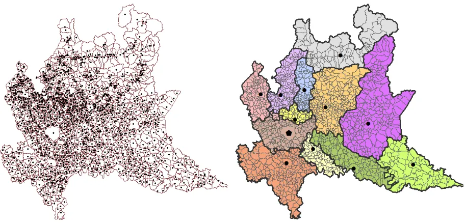
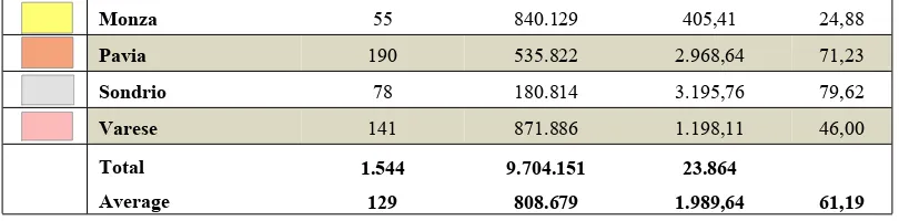
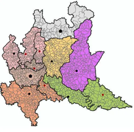
The proposed models were tested on a case study concerning the largest Italian region. Lombardia is the most populated region in Italy (almost 10 million inhabitants), characterized by a remarkable number of municipalities (1544 territorial units) currently grouped in 12 provinces (districts) (see Figures 3 and 4). The region is involved in the general reorganization process described in Section 2; Table 4 provides a description of the current configuration, reporting, for each province , the number of territorial units, the total � population, the area and the radius ��� (i.e. the distance between the province chief town and the farthest municipality assigned to it).
Population data for each unit comes from the most recent census figures (ISTAT, 2011), while distances among municipalities have been calculated as shortest routes (in km) on the road network (considering motorways, national and regional roads).
[image:12.595.75.532.344.564.2]Considering the current configuration (Table 4), only three provinces (Bergamo, Brescia and Pavia) satisfy both the feasibility requirements imposed by the government (i.e. minimum area of 2500 km2 and minimum population of 350.000 inhabitants). Therefore, a reduction in the total number of districts might produce a more efficient solution.
Figure 3 – Municipalities of Lombardia region Figure 4 –Provinces (and related municipalities) of Lombardia region
Districts (Provinces)
Territorial units
(Municipalities) Population
Area (km2)
Rmj (km)
Provinc
B Bergamo 244 1.086.277 2.745,94 65,63
B Brescia 206 1.238.044 4.785,62 114,68
C Como 160 586.735 1.279,04 63,12
C Cremona 115 357.623 1.770,46 65,13
LeLecco 90 336.310 814,58 41,84
nte L Lodi 61 223.755 782,99 43,33
nte
MMantova 70 408.336 2.341,44 59,64
[image:12.595.96.500.606.762.2]MMonza 55 840.129 405,41 24,88
P Pavia 190 535.822 2.968,64 71,23
SSondrio 78 180.814 3.195,76 79,62
V Varese 141 871.886 1.198,11 46,00
Total 1.544 9.704.151 23.864
Average 129 808.679 1.989,64 61,19
[image:13.595.96.501.73.173.2]* Regional Chief Town
Table 4 – Characteristics of the case study of Lombardia region
5.1 Models Results
The described case study was utilized as a test problem, in order to analyze the solutions provided by the four proposed models, also comparing these to both the current configuration and the governmental proposal. It must be noted that, in all models, Milano was labeled as “special district”, due to its role of regional chief town, along with Sondrio, due to the physical characteristics of its territory (mainly composed of Alpine areas and therefore not suitable for mergers with other areas of the region).
Each model has been optimally solved using IBM ILOG Cplex 12.2 on an Intel Core i7 with 1.86 GHz and 4 GB of RAM. Each provided solution has been represented on a map through a linkage with a GIS. All models have been applied without the inclusion of explicit contiguity constraints. Hence, contiguity conditions have been assessed a posteriori, through the support of the GIS; and solutions have been heuristically modified in presence of non-contiguities.
In the following, the results provided by each model are examined and discussed. In particular, we first consider the solutions obtained by the prescriptive models and then those by the optimal ones. Finally, solutions are compared among themselves and to the one proposed by the government.
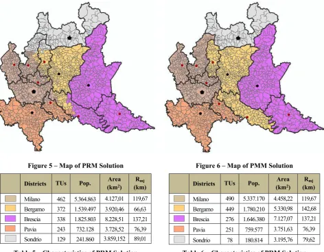
Prescriptive Models
Figure 5 – Map of PRM Solution Figure 6 – Map of PMM Solution
Districts TUs Pop. Area (km2)
Rmj (km)
V Milano 462 5.364.863 4.127,01 119,67 T Bergamo 372 1.539.497 3.920,46 66,63
B Brescia 338 1.825.803 8.228,51 137,21 A Pavia 243 732.128 3.728,52 76,39 S Sondrio 129 241.860 3.859,152 89,01
Districts TUs Pop. Area (km2)
Rmj (km)
V Milano 490 5.337.170 4.458,22 119,67 T Bergamo 449 1.780.210 5.330,98 142,68
B Brescia 276 1.646.380 7.127,07 137,21
A Pavia 251 759.577 3.751,63 76,39
S Sondrio 78 180.814 3.195,76 79,62
Table 5 – Characteristics of PRM Solution Table 6 – Characteristics of PRM Solution
The two solutions are characterized by a very limited number of provinces covering very wide areas. In particular, the resulting Bergamo and Brescia districts account for wide areas and a very large Rmj value.
Optimal Models
[image:14.595.64.537.70.438.2]Figure 7 – Map of ORM solution (k=kmin=5) Figure 8 – Map of OMM solution (k=kmin=5)
Districts TUs Pop. Area (km2)
Rmj (km)
V Milano 210 3.930.781 2.229,94 62,26 T Bergamo
344 1.427.265 3.657,61 65,63 Br Brescia 238 1.366.144 5.378,33 114,68 A Pavia 242 729.441 3.718,09 76,39
nte
M Mantova 100 459.659 2.850,18 64,48 S Sondrio 106 212.596 3.521,77 79,62
V Varese
304 1.578.265 2.507,74 85,42
Districts TUs Pop. Area (km2)
Rmj (km)
V Milano 189 3.878.549 1.981,07 59,23 T Bergamo 244 1.086.277 2.745,94 65,63
Br Brescia 206 1.238.044 4.785,62 114,68 A Pavia 251 759.577 3.751,63 76,39 C Cremona 185 765.959 4.111,90 123,81 S Sondrio 78 180.814 3.195,76 79,61
V Varese 391 1.794.931 3.291,73 97,01
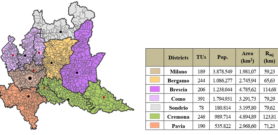
[image:15.595.56.291.75.300.2] [image:15.595.309.542.82.312.2] Comparison with the governmental proposal
As shown in Figure 3, Italian Government proposed a reorganization of the districts for each single region. Starting from the principle that infeasible provinces should be suppressed (apart the ones labeled as “special districts”), new provinces have been obtained by merging the current ones. This proposal has been obtained by performing, for each region, ad hoc considerations, also taking into account local political factors.
[image:16.595.78.527.230.448.2]Figure 9 shows the governmental proposal for Lombardia. The following mergers are performed: Milano with Monza; Varese with Como and Lecco; Cremona with Mantova and Lodi. Sondrio, Bergamo, Brescia and Pavia remain unchanged.
Figure 9 – Government Proposal (k= 5)
Districts TUs Pop. Area (km2)
Rmj (km)
V Milano 189 3.878.549 1.981,07 59,23 T
Bergamo 244 1.086.277 2.745,94 65,63 B Brescia 206 1.238.044 4.785,62 114,68 C Como 391 1.794.931 3.291,73 79,29
S Sondrio 78 180.814 3.195,80 79,62 C Cremona 246 989.714 4.894,89 123,81 A Pavia 190 535.822 2.968,60 71,23
Table 9 – Government Proposal (k= 5)
Comparing this solution to the ones provided by optimal models (Figures 7 and 8), many similarities can be noticed, especially with the one provided by the OMM. In this case, the main differences consist in the assignment of the province of Lodi (merged with Pavia instead of Mantova and Cremona) and in the choice of the chief town for the new province of Varese-Como-Lecco (located in Varese instead of Como). The choices of the model seem to be reasonable and produce more compact districts. Indeed, the centroid of the province of Lodi is closer to the chief town of Pavia than to the one of Cremona; moreover, the choice of Varese as chief town for the new Varese-Como-Lecco province guarantees a more compact solution in term of weighted distance.
On the other hand, the solution of the ORM (with �= 5) is the best one in terms of compactness (due to the possibility of reassigning single territorial units).
Decision making implications
The proposed models can be used as useful decision support tool for policy makers, as they allow producing multiple scenarios (by varying calibration parameters) that may be compared across appropriate indicators.
An example of this possible usage of the models is shown in the following, where a scenario analysis is performed by varying the number of districts to be suppressed. Results are � compared across the following indicators:
average, minimum and maximum values for Area, Population, Number of Territorial Units and Radius per district;
the Population (Area) Variance Index VARpop (VARsup,), i.e. the mean square deviation of
the population (area) of the new provinces from the average population (area) value. This index can be assumed as a proxy of the uniformity of the population (area) distribution across resulting provinces.
the Compactness index (Ic), defined as the weighted average distance between a single
user/citizen and its assigned chief town:
�� =
∑
� ∈ �� ∈ �
∑
���������∑
� ∈ ��� the Hoover Index (IH), defined as half of the sum of the differences between the
percentages of population and area of each province:
�� = 1
2∙
∑
j∈J
|
Pj
� -
Sj
S
|
* 100where and are the total population and area of the region. This index is generally used � � to evaluate population distribution across a set of districts (Long and Nucci, 1997); the population is considered to be fairly distributed if provinces account for similar shares of population and areas (for instance, a province accounting for 10% of the regional population should also account for 10% of the area). This way, gets closer to 0; on the I
H
contrary, gets closer to 100 as unbalances in population distribution grow. IH
Tables 10a and 10b report the values of the indicators provided by the proposed models, by varying the number of provinces to be closed (from the minimum feasible value � �= 5 to
, i.e. the number of districts closed by the prescriptive models).
�= 7
Population(inhabitants) 103 Area(km2) Active
Districts Avg Min Max
VARpop (106)
Avg Min Max
VARarea (103)
Current Configuration 12 808 180 3.038 0,78 1.988 405 4.785 1,27
Governmental Proposal 7 1.386. 180 3.878 1,21 3409 1.981 4.894 1,07
ORM (k=5) 7 1.386 212 3.930 1,24 3.409 2.229 5.378 1,05
OMM (k=5) 7 1.386 180 3.878 1,21 3.409 1.981 4.785 0,92
ORM (k=6) 6 1.617 214 4.649 1,59 3.977 2.500 5.792 1,35
OMM (k=6) 6 1.617. 180 4.638 1,57 3.977 2.745 5.732 1,13
ORM (k=7) 5 1.940 241 6.080 2,38 4.772 2.850 7.704 1,88
PRM (k=7) 5 1.940. 241 5.364 2,02 4.772 3.728 8.228 1,94
OMM (k=7) 5 1.940 180 4.638 1,64 4.772 3.195 7.127 1,67
PMM (k=7) 5 1.940 180 5.337 2,01 4.772 3.195 7.127 1,54
Number of territorial units Radius (km) Active
Districts Avg Min Max
Average Distance ��
(km) Avg Min Max
Hoover Index ��
Current Configuration 12 129 55 244 17,28 61 24 114 36,37
Governmental Proposal 7 221 78 391 24,34 84 59 123 36,37
ORM (k=5) 7 221 100 344 21,67 78 62 114 36,9
OMM (k=5) 7 221 78 391 23,93 88 59 123 36,4
ORM (k=6) 6 257 100 444 23,28 85 64 114 29,5
OMM (k=6) 6 257 78 440 25,46 98 65 123 28,5
ORM (k=7) 5 309 100 695 26,48 90 64 119 30,4
PRM (k=7) 5 309 129 462 27,73 97 66 137 38,0
OMM (k=7) 5 309 78 440 27,80 113 79 142 28,5
PMM (k=7) 5 309 78 490 28,86 111 76 142 36,3
Tables 10a (top) and 10b (bottom) – Comparison of the solutions provided by the models
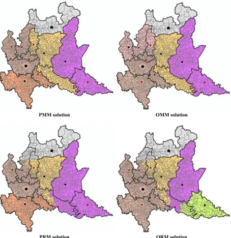
As an example, scenarios with five active districts are discussed (see the last rows of Tables 10 - corresponding to �= 7 - and Figure 10) in order to compare results provided by the model.
In this case, solutions are characterized by large districts with an average population of almost 2 millions of inhabitants and an average area of about 5000 km2. As expected, the
PMM solution OMM solution
[image:19.595.75.530.70.539.2]PRM solution ORM solution
Figure 10 – Comparison of solutions provided by the models for k=7
6. Conclusions
In recent years, mainly due to austerity measures, central and local authorities in many countries have been involved in the rationalization and reorganization of systems providing essential public services. Consequently, due to the territorial organization of such services, many actions concerning the restructuring of local government administrative units have been undertaken, with the objective of reducing associated costs. Specifically, in Italy there have been several reform proposals aimed at merging and rearranging current territorial administrative units, such as provinces.
how models provide solutions with different characteristics and performances. In particular, by appropriately combining calibration parameters, models can provide a wide set of alternative territorial configurations to be analyzed and considered. Also, such configurations have been compared to governmental proposals, through the introduction of a set of appropriate indicators, highlighting how models can produce significantly better outcomes for the amalgamation process. Choices provided by the models are reasonable and produce more compact districts.
Further researches will be addressed at enhancing the models formulations in order to take into account further characteristics (such as balancing or political constraints) that may help in producing further attractive solutions for policy makers.
References
Allers, M.A., Geertsema, J.B (2016). The effects of local government amalgamation on public spending, taxation and service levels: evidence from 15 years of municipal consolidation. Journal of Regional Science, forthcoming.
Andrews, R., Boyne, G. (2012). Structural change and public service performance: The impact of the reorganization process in English local government. Public Administration, 90(2), 297-312.
Bolgherini, S. (2014) Can austerity lead to recentralisation? Italian local government during the economic crisis. South European Society and Politics 19(2), 193-214.
Boyne, G. A., Cole, M. (1998). Revolution, evolution and local government structure: an empirical analysis of London. Urban Studies, 35(4), 751-768.
Bozkaya, B., Erkut, E., Laporte, G. (2003). A Tabu Search heuristic and adaptive memory procedure for political districting. European Journal of Operational Research, 144, 12–26.
Browdy, M. H. (1990). Simulated annealing: an improved computer model for political redistricting. Yale Law & Policy Review, 163-179.
Byfuglien, J., Nordgard, A. (1973). Region-building: A comparison of methods. Norwegian Journal of Geography, 27:127–151.
Corriere della Sera (2013). Government tries again to abolish provinces. Available online at: http://www.corriere.it/International/english/articoli/2013/07/05/government.shtml?ref resh_ce-cp [Last accessed on 24th May 2016]
D'Amico, S. J., Wang, S. J., Batta, R., Rump, C. M. (2002). A simulated annealing approach to police district design. Computers & Operations Research, 29(6), 667-684.
Denhardt, R., Denhardt, J., Blanc, T. (2013). Public administration: An action orientation. Cengage Learning.
Duque, J. C., Ramos, R., Suriñach, J. (2007). Supervised regionalization methods: A survey. International Regional Science Review, 30(3), 195-220.
EUROSTAT (2002). European Regional Statistics. Changes in the NUTS Classifications,
1981-1999. Available online at:
http://ec.europa.eu/eurostat/documents/345175/629341/NUTS+1981-1999. [Accessed on 30 July 2013].
Gazzetta Ufficiale (2012). Determinazione dei criteri per il riordino delle province. Available online at: http://www.gazzettaufficiale.it/eli/id/2012/11/06/012G0210/sg (in Italian). Gazzetta Ufficiale (2014). Disposizioni sulle citta' metropolitane, sulle province, sulle unioni
e fusioni di comuni. Serie Generale. Available online at: http://www.gazzettaufficiale.it/eli/id/2014/4/7/14G00069/sg (in Italian).
George, J.A., Lamar, B.W., Wallace, C.A. (1997). Political district determination using large-scale network optimization. Socio-Economic Planning Sciences, 31(1):11-28.
Hanafi, S., Freville, A., Vaca, P. (1999). Municipal solid waste collection: An effective data structure for solving the sectorization problem with local search methods. INFOR J.,
37(3), 236-254.
Hess, S.W., Weaver, J.B., Siegfeldt, H.J., Whelan, J.N., Zitlau, P.A (1965). Nonpartisan Political Redistricting by Computer. Operations Research, 13(6), 998-1006.
Hojati, M. (1996). Optimal political districting. Computers & Operations Research, 23(12), 1147-1161.
Kalcsics, J. (2015). Districting Problems. In: Laporte, G., Nickel, S., Saldanha da Gama, F. (Eds.) Location Science (pp. 595-622). Springer International Publishing.
ISTAT (2011). Dati del Censimento Generale della Popolazione Italiana (National Census Data). Available online at: http://censimentopopolazione.istat.it/default.html, last accessed on 30August 2013.
Jakobsen, M., Kjaer, U. (2016) Political Representation and Geographical Bias in Amalgamated Local Governments, Local Government Studies, 42:2, 208-227.
Leach, S. (2009). Reorganisation, Reorganisation, Reorganisation: A Critical Analysis of the Sequence of Local Government Reorganisation Initiatives, 1979–2008. Local Government Studies, 35(1), 61-74.
Long, L., Nucci, A. (1997). The Hoover index of population concentration: A correction and update. The Professional Geographer, 49(4), 431-440.
Maravalle, M., Simeone, B. (1995). A spanning tree heuristic for regional clustering. Communications in Statistics-Theory and Methods, 24:625– 639.
Mehrotra, A., Johnson, E.L., Nemhauser, G.L. (1998). An optimization based heuristic for political districting. Management Science, 44(8):1100-1114.
Meligrana, J. (Ed.). (2005). Redrawing local government boundaries: an international study of politics, procedures, and decisions. UBC Press
Oates, W.E. (1972). Fiscal Federalism. New York: Harcourt, Brace and Jovanovich.
Ricca, F., Simeone, B. (2008). Local search algorithms for political districting. European Journal of Operational Research, 189(3), 1409-1426.
Ricca, F., Scozzari, A., Simeone, B., (2011). Political districting: from classical models to recent approaches. 4OR, 9, 223-254.
Schoepfle, O.B., Church, R.L (1991). A new network representation of a classic school districting problem. Socio-Economic Planning Sciences, 25(3):189-197.
Teles, F. (2016). In Search of Efficiency in Local Governance: Size and Alternatives. In Local Governance and Inter-municipal Cooperation, 32-49. Palgrave Macmillan UK.
Wise, S., Haining, R., Ma., J. (1997). Recent developments in spatial analysis: Spatial statistics, behavioural modelling, and computational intelligence, chapter Regionalisation tools for exploratory spatial analysis of health data. Edited by Manfred M. Fischer and Arthur Getis, pages 83–100. Springer, New York.
Warner, M.E. (2010). The Future of Local Government: Twenty-First-Century Challenges.
Public Administration Review, 70, 145-147.
Williams, J.C. (1995). Political redistricting: a review. Papers in Regional Science, 74(1), 13-40.
Giuseppe Bruno
Giuseppe Bruno is Associate Professor in Operational Research and Decision Science
Methodologies at University of Naples “Federico II”. He holds a PhD in Computer Science and Robotics (University of Naples Federico II, 1994). He is a Member of the Italian Association of Operational Research (AIRO), of the European Working Group on Locational Analysis, and of the European Working Group on Transportation. His main research interests are in the fields of Locational analysis, Logistics, Transportation, Multi-Criteria Decision-Making Analysis. His research has appeared on prestigious international journals.
Andrea Genovese
Andrea Genovese holds a PhD in Science and Technology Management from the University of Naples ‘Federico II’ (Italy) and a MBA from Whittemore School of Business and Economics at University of New Hampshire (USA). Since 2010, he has been working at the University of Sheffield Management School (UK), where he is currently a Senior Lecturer in Logistics and Supply Chain Management. His research interests include the development of Decision Support Models for Supply Chain and Logistics Problems (with emphasis on Green and Sustainability issues) along with Multi-Criteria Decision-Making problems. His research has appeared on prestigious international journals.
Carmela Piccolo
Carmela Piccolo is a research fellow at University of Naples Federico II (Italy). She received her PhD in the area of Operational Research, at University of Naples "Federico II". Her research interests focus on the field of optimization models in the context of the territorial organization of services (districting and facility location problems) and of the multi-criteria decision-making processes. She has significant expertise in GIS and location theory.