https://doi.org/10.5194/esd-8-617-2017
© Author(s) 2017. This work is distributed under the Creative Commons Attribution 3.0 License.
Flexible parameter-sparse global temperature time
profiles that stabilise at 1.5 and 2.0
◦
C
Chris Huntingford1, Hui Yang2,1, Anna Harper3, Peter M. Cox3, Nicola Gedney4, Eleanor J. Burke5, Jason A. Lowe5, Garry Hayman1, William J. Collins6, Stephen M. Smith7, and Edward Comyn-Platt1
1Centre for Ecology and Hydrology, Benson Lane, Wallingford, Oxfordshire, OX10 8BB, UK
2Department of Ecology, School of Urban and Environmental Sciences, Peking University, Beijing, 100871,
P.R. China
3College of Engineering and Environmental Science, Laver Building, University of Exeter, North Park Road,
Exeter, EX4 4QF, UK
4Met Office Hadley Centre, Joint Centre for Hydrometeorological Research, Maclean Building, Wallingford,
OX10 8BB, UK
5Met Office, FitzRoy Road, Exeter, Devon, EX1 3PB, UK
6Department of Meteorology, University of Reading, Earley Gate, P.O. Box 243, Reading, RG6 6BB, UK
7Committee on Climate Change, 7 Holbein Place, London, SW1W 8NR, UK
Correspondence to:Chris Huntingford ([email protected])
Received: 24 February 2017 – Discussion started: 2 March 2017 Accepted: 29 May 2017 – Published: 14 July 2017
Abstract. The meeting of the United Nations Framework Convention on Climate Change (UNFCCC) in
1 Introduction
The conventional approach to understand climate change for possible futures is to force Earth system models (ESMs) with either emissions scenarios (e.g. Cox et al., 2000) or prescribed future atmospheric greenhouse gas (GHG) con-centrations (e.g. Meinshausen et al., 2011). However, recent UNFCCC meetings have placed a focus on prescribed tem-perature thresholds. This has mainly focused on how to avoid crossing 2.0◦C of global warming since pre-industrial times. Furthermore, the December 2015 Paris Conference of the Parties (COP21) meeting suggested an additional aspiration of remaining below a 1.5◦C warming threshold. To achieve the latter could in particular involve major changes in energy demand or production (Rogelj et al., 2013) and extensive re-liance on artificial carbon removal (Fuss et al., 2014) such as biofuels combined with carbon capture and storage. Equi-librium temperatures associated with even current GHG con-centrations may already correspond to warming levels near 1.5◦C (Huntingford and Mercado, 2016). Therefore, given the likely difficulty of fulfilling the 1.5◦C target, there is a focus on understanding what is to be gained climatically from achieving that lower threshold and the impacts of any temporary overshoot beforehand. There is a related need to calculate the amount of flexibility between different mixtures of greenhouse gas emissions that will achieve the same even-tual stabilisation levels. Forward modelling by prescription of emissions or GHG concentrations cannot answer these questions directly, as there is no guarantee that a particular simulation will asymptote precisely to an increase of 1.5 or 2.0◦C. Instead, climate modelling needs to develop inversion methods that follow predefined future warming profiles. Ex-isting ESM projections (e.g. from the CMIP5 database; Tay-lor et al., 2012) can be scaled to these, for instance by pattern scaling (e.g. Huntingford and Cox, 2000). Here we move towards that by presenting families of temperature profiles that eventually stabilise. The use of common future warming trajectories may lead to easier discussion and comparison be-tween projects designed to assess a range of implications of either the 1.5 or 2.0◦C target.
2 Temperature profiles that asymptote to prescribed
temperature limits
2.1 One-parameter profiles
Derived are profiles of global warming above pre-industrial levels,1T(t) (◦C), dependent on timet (yr) and witht=0 as year 2015. Three boundary conditions are satisfied, with two related to present-day warming. One is an estimate of warming between pre-industrial times and the year 2015, 1T0 (◦C). The second is an estimate of the current rate
of global warming, β=d1T /dt|t=0 (◦C yr−1). The values of these two parameters are derived from the HadCRUT4 dataset (Morice et al., 2012). We use the median from the
100 HadCRUT4 decadally-smoothed realisations of global temperature rise estimates (see Data Availability below; Had-CRUT4 smoothing is with a 21-point binomial filter applied to annual values). Values in that dataset normalise against the period 1961–1990; we renormalise to the period 1850–1900 as a proxy for pre-industrial times, giving1T0=0.89◦C.
For further discussion of this value, see Hawkins et al. (2017). The recent gradient in warming is from regression fitting of the last 21 years (1995–2015 inclusive), giving β=0.0128◦C yr−1. We note, though, that when using Had-CRUT4 as our observationally based starting point, it is nec-essary to be aware of its non-global spatial extent. Addition-ally, it is compiled from a mix of air and sea surface tempera-tures, as described in Cowtan et al. (2015). The third bound-ary condition is the final prescribed warming level1TLim
(◦C), i.e. 1.5 or 2.0◦C. This is an eventual stabilisation level that our profiles1T approach asymptotically. The specifica-tion of the temperature thresholds in the COP21 statements could have other interpretations, including eventual stabilisa-tion at even lower warming levels or long-term temperature fluctuations, but which remain below prescribed limits. We do however allow the possibility of a near-term temporary overshoot of1TLim, as described below.
We search for a parameter-sparse family of curves and consider a path that moves away from a linear temperature rise (via parameterγ) and towards a stabilisation level. Char-acterising different curves with an adaptation parameter µ (yr−1) leads to
1T =1T0+γ t− 1−e−µt γ t−(1TLim−1T0). (1)
A larger (positive) value forµrepresents greater societal ca-pability to adjust the temperature pathway towards a stable temperature state. The value of 1/µ(yr) is an approximatee -folding time in moving from a non-zero positive gradient (in time) of global warming and towards levelling off at1TLim.
Taking the time derivative of Eq. (1) (Appendix, Eq. A2) and matching to the historical record at yeart=0 gives
γ=β−µ(1TLim−1T0). (2)
Hence, γ is not the current rate of warming, i.e. γ6=β. From Eq. (A4) and for 0< µ <2β/(1TLim−1T0), this
gives d21T /dt2|t=0<0.0, corresponding to no acceleration of the warming rate in the immediate future. Solutions re-quireµ >0 for convergence.
Profiles for different µ values and for 1TLim values of
0 50 100 150 200 250 300
Years since 2015 (yr)
0.6 0.8 1.0 1.2 1.4 1.6 1.8 2.0 2.2
Gl
ob
al
wa
rm
ing
si
nc
e p
re
-in
du
str
ial
(
◦C)
µ=0.05 yr−1
µ=0.03 yr−1
µ=0.0074 yr−1
Historical trend
Pathways to 2.0◦C
0 50 100 150 200 250 300
Years since 2015 (yr)
0.6 0.8 1.0 1.2 1.4 1.6 1.8 2.0 2.2
µ=0.05 yr−1
µ=0.03 yr−1
µ=0.0074 yr−1
Historical trend
[image:3.612.116.482.64.223.2]Pathways to 1.5◦C
Figure 1.The effect of changingµin the single-parameter temperature profiles, designed to asymptote to either 2.0◦C (left panel) or 1.5◦C (right panel). Values ofµas given in the legend.
0 50 100 150 200 250 300
Years since 2015 (yr)
0.6 0.8 1.0 1.2 1.4 1.6 1.8 2.0 2.2
Gl
ob
al
wa
rm
ing
si
nc
e p
re
-in
du
str
ial
(
◦C)
µ0=0.05 yr−1, µ1=0.0004 yr−2
µ0=0.03 yr−1, µ1=0.0 yr−2
µ0=0.0012 yr−1, µ1=0.0001 yr−2
Historical trend
Pathways to 2.0◦C
0 50 100 150 200 250 300
Years since 2015 (yr)
0.6 0.8 1.0 1.2 1.4 1.6 1.8 2.0 2.2
µ0=0.05 yr−1, µ1=0.0004 yr−2
µ0=0.03 yr−1, µ1=0.0 yr−2
µ0=0.0012 yr−1, µ1=0.0001 yr−2
Historical trend
Pathways to 1.5◦C
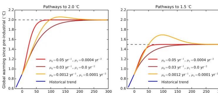
Figure 2.The effect of changingµ0andµ1in the two-parameter temperature profiles, designed to asymptote to either 2.0◦C (left panel) or
1.5◦C (right panel). Values ofµ0andµ1as given in the legend.
2.2 Two-parameter profiles
Whilst aiming to create profiles that are simple and math-ematically tractable, allowing just one parameter may be overly restrictive. For example, society might be much more able to reduce emissions (corresponding to high µ values) further in the future, but may be less able to in the near future. To capture differences in generational approaches to fossil fuel usage, one additional degree of freedom is introduced, settingµ(t) as a function of time:
µ(t)=µ0+µ1t. (3)
Matching the first derivative (Appendix, Eq. A6) at yeart= 0 gives
γ =β−µ0(1TLim−1T0). (4)
Profiles for different µ0 (yr−1) andµ1 (yr−2) values are
presented in Fig. 2. Curves can approach the warming tar-get rapidly, then quickly asymptote to it through an increas-ingly large value in time ofµ(e.g. red curve, 2.0◦C target).
Similarly, increasingµvalues offer the opportunity to have overshoot occurrences followed by rapid convergence to the desired warming level (e.g yellow curve, 1.5◦C target).
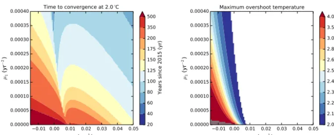
The left-hand panel in Fig. 3 presents the time from the year 2015 to achieve stabilisation, defined as within 0.01◦C of the target temperature threshold of 2.0◦C. The right-hand panel shows the maximum additional overshoot tempera-ture should1TLimbe crossed. Figure 4 shows the same for 1TLim=1.5◦C. These look-up charts enable the selection
of a balance between general action on moving away from a business-as-usual approach to emissions (via parameterµ0)
and leaving more change to future generations (via parame-terµ1). Lowerµ0andµ1values take longer to reach
[image:3.612.114.485.271.430.2]0.01 0.00 0.01 0.02 0.03 0.04 0.05 µ0 (yr−1)
0.00000 0.00005 0.00010 0.00015 0.00020 0.00025 0.00030 0.00035 0.00040 µ1 (y r − 2)
Time to convergence at 2.0◦C
20 40 60 80 100 125 150 175 200 350 500
Years since 2015 (yr)
0.01 0.00 0.01 0.02 0.03 0.04 0.05 µ0 (yr−1)
0.00000 0.00005 0.00010 0.00015 0.00020 0.00025 0.00030 0.00035 0.00040 µ1 (y r − 2)
Maximum overshoot temperature
2.0 2.1 2.2 2.3 2.4 2.5 2.6 2.8 3.0 3.5 4.0
Maximum temperature where overshoot
[image:4.612.131.468.64.200.2]of 2 .0 ◦C oc cu rs ( ◦C)
Figure 3.The dependence of the time to stabilisation and any overshoot magnitude (where present, white space otherwise) on the parameters µ0andµ1in the temperature profiles, with1TLim=2.0◦C. The scale of the colour bar is nonlinear. The grey region in the bottom left
corner of the right-hand panel is where temperatures become higher than the target of 2.0◦C and increase throughout the 500 years; thus, peak warming is not attained in that time.
0.01 0.00 0.01 0.02 0.03 0.04 0.05 µ0 (yr−1)
0.00000 0.00005 0.00010 0.00015 0.00020 0.00025 0.00030 0.00035 0.00040 µ1 (y r − 2)
Time to convergence at 1.5◦C
20 40 60 80 100 125 150 175 200 350 500
Years since 2015 (yr)
0.01 0.00 0.01 0.02 0.03 0.04 0.05 µ0 (yr−1)
0.00000 0.00005 0.00010 0.00015 0.00020 0.00025 0.00030 0.00035 0.00040 µ1 (y r − 2)
Maximum overshoot temperature
1.5 1.6 1.7 1.8 1.9 2.0 2.1 2.3 2.5 3.0 3.5
Maximum temperature where overshoot
[image:4.612.130.469.269.404.2]of 1 .5 ◦C oc cu rs ( ◦C)
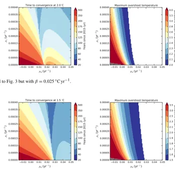
Figure 4.The dependence of the time to stabilisation and any overshoot magnitude (where present, white space otherwise) on the parameters µ0andµ1in the temperature profiles, with1TLim=1.5◦C. The scale of the colour bar is nonlinear. The grey region in the bottom left
corner of the right-hand panel is where temperatures become higher than the target of 1.5◦C and increase throughout the 500 years; thus, peak warming is not attained in that time.
target level. By definition, solutions ofµ0<0.0 andµ1=0
never converge.
One potential evolution of global temperature could be a rapid rise to 2.0◦C of global warming, followed by strong efforts to quickly reduce and stabilise at 1.5◦C. To achieve this on a single-century timescale, with the curve structure of Eqs. (1) and (3) and1TLim=1.5◦C,µ0must be slightly
negative, combined with high values ofµ1. This influences
the selection of the ranges ofµ0andµ1in Fig. 4.
2.3 Fitting to existing ESM simulations
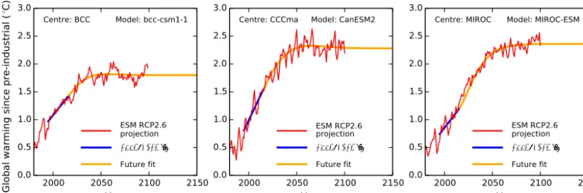
Equations (1), (3) and (4) generate a range of future tem-perature pathways towards prescribed warming limits. For these, the related changes in atmospheric gas concentrations and emissions can be determined. However, many ESMs have been operated in forward mode, forced with scenar-ios of atmospheric GHG concentrations that correspond to heavy mitigation of fossil fuel burning. The RCP2.6 scenario (Meinshausen et al., 2011) gives ESM-based estimates of the
stabilisation of global warming around 2.0◦C warming since pre-industrial times. We fit our model to these ESM pro-jections of the RCP2.6 scenario. Parametersβ and1T0are
tuned to their projections of temperature for the years 1995– 2015, whilst1TLim,µ0andµ1are fitted to the years 2016–
2000 2050 2100 2150
Year
0.0 0.5 1.0 1.5 2.0 2.5 3.0
Gl
ob
al
wa
rm
ing
si
nc
e p
re
-in
du
str
ial
(
◦
C)
Centre: BCC Model: bcc-csm1-1
Future fit
1995–2015 fit
ESM RCP2.6
projection
2000 2050 2100 2150
Year
0.0 0.5 1.0 1.5 2.0 2.5 3.0
Centre: CCCma Model: CanESM2
Future fit
1995–2015 fit
projection
2000 2050 2100 2150
Year
0.0 0.5 1.0 1.5 2.0 2.5 3.0
Centre: MIROC Model: MIROC-ESM
Future fit 1995–2015 fit projection
[image:5.612.87.512.68.209.2]ESM RCP2.6 ESM RCP2.6
Figure 5.Fit of Eq. (1) (oranges curves) for the years after 2015 and for three representative ESM simulations (red curves) that correspond to the RCP2.6 scenario of atmospheric gas changes. The blue curve is the linear fit to the ESM for the period 1995–2015. Annotated in each panel is the modelling centre and the ESM name. The fit to all the RCP2.6 simulations is given in Fig. B1.
We additionally fit our curves to pathways in which the emissions are generated using integrated assessment models (IAMs) and the related global temperature profiles are cre-ated using a simple climate model. This has been done for warming profiles from the IPCC scenario database (https: //tntcat.iiasa.ac.at/AR5DB/) and for the marker scenarios of the more recent shared socioeconomic pathways (SSPs) database (https://tntcat.iiasa.ac.at/SspDb). We demonstrate that the functional forms used here can also represent these IAM-based scenarios to a good level of accuracy (see the Supplement).
2.4 Accounting for uncertainty in warming rates
The relatively low rate of warming increase since the year 1998 has been the subject of debate and is sometimes re-ferred to as the “warming hiatus”. The possibility of such a warming hiatus occurring has been assessed in detail (e.g. Roberts et al., 2015). If a natural decadal-timescale fluctu-ation has temporarily suppressed the background warming trend, then our HadCRUT-based warming rateβcould be too small. The MAGICC climate impacts model, parameterised against a range of ESMs, typically projects the recent warm-ing as around β=0.025◦C yr−1. As a sensitivity study, we
reproduce Figs. 3 and 4 using that higher warming rate as Figs. B2 and B3, respectively.
2.5 Applications
Our profiles enable a common framework for the discussion of warming trajectories that stabilise to predefined tempera-ture limits. Regional climate change corresponding to these global temperatures can be estimated from interpolation of ESM projections (e.g. by pattern scaling; Huntingford and Cox, 2000). Such scaling techniques can be linked to im-pact models (e.g. Huntingford et al., 2010). In the com-prehensive review of methods for identifying regional dif-ferences associated with alternative global warming targets,
James et al. (2017) note pattern scaling as a key technique. The accuracy of this interpolation system has been recently reviewed in detail by Tebaldi and Arblaster (2014) and with enhancements proposed by Herger et al. (2015). In the other approaches of James et al. (2017), the central issue of how to interpret existing simulations, which even for identical forc-ings, project a range of different future final warming levels, remains.
Emissions profiles can be calculated to fulfil the ESM-dependent radiative forcings associated with any prescribed global temperature stabilisation profile. These can include different mixtures of individual GHG emissions, whilst ac-counting for any perturbed land–atmosphere and ocean– atmosphere gas exchanges. The sum of the radiation changes for altered individual atmospheric greenhouse gas combina-tions must equal the ESM-dependent radiative forcing. Al-though our analytical forms are generic and can be calcu-lated for any prescribed final stabilised temperature1TLim,
the emphasis here is placed on the 1.5 or 2.0◦C targets. This is due to their strong current discussion in policy circles re-garding clean energy (e.g. Obama, 2017).
3 Conclusions
Presented in this work are parameter-sparse algebraic curves that match contemporary levels and the rate of change of global mean temperature and that asymptote to prescribed warming thresholds. These represent a smooth transition from current rates of warming through to stabilised tempera-ture levels. They can include an initial overshoot of temper-atures above any desired final warming level. Their relative simplicity makes them transparent and open to discussion. If common temperature scenarios are adopted by a range of studies (by selection ofµ0,µ1and1TLimvalues), this may
allow easier comparison of either the impacts of or emissions to achieve 1.5 or 2.0◦C warming stabilisation. At this stage, we do not associate any particular parameter combinations (or ranges) with their feasibility of fulfilment by society.
The curves have five parameters, with three of these con-strained by the current warming level1T0, the current rate of
warming changeβand the final stabilised state1TLim. The
remaining two parametersµ0andµ1, offering two degrees of
freedom, give flexibility to the pathway shape before asymp-toting to the temperature 1TLim. Our curves allow for the
possibility of temporary overshoot. This enables the charac-terisation of the illustrative scenarios proposed in Schneider and Mastrandrea (2005, Fig. 4), and their metric of dangerous anthropogenic interference (DAI) defined as the integrated time and magnitude spent overshooting a safe upper limit. Where an impact study is for a period ahead that is much less than the time to stabilisation, then these curves allow for the possibility of gradually rising or declining temperatures through any analysis period.
Some very specific pathways may require further versa-tility. For instance, defining a pathway asymptoting to 1.5◦C and allowing warming overshoot to 2.0◦C constrains one de-gree of freedom. If the difference between the speed of ap-proaching 2.0◦C is specified as either much quicker or much slower than the time from that peak to 1.5◦C, then two more degrees of freedom are required, giving three in total. To sat-isfy situations such as this, further curve forms could, for in-stance, include specification ofµas a quadratic function of time.
Code availability. The Python scripts leading to any of
the diagrams are available on request to Chris Huntingford ([email protected]).
Data availability. The global warming amount to the present
Appendix A: First and second derivatives
Here we present the first and second derivatives for the one-and two-parameter profiles.
A1 One-parameter profiles The first derivative of Eq. (1) satisfies
d1T
dt =γ− 1−e
−µt γ
−−e−µt·(−µ)
·γ t−(1TLim−1T0), (A1)
which, att=0, gives
d1T
dt |t=0=β=γ+µ 1TLim−1T0
. (A2)
The second derivative of Eq. (1) is found by differentiating Eq. (A1) with respect tot, giving
d21T
dt2 = −(−e
−µt· −µ) γ
−−e−µt· −µ γ
−−e−µt·(−µ)·(−µ)·γ t−(1TLim−1T0)
= −2µγ e−µt+µ2e−µt
γ t−(1TLim−1T0),
which, at timet=0, gives
d21T
dt2 |t=0= −2µγ−µ 2(1T
Lim−1T0). (A3)
Substitution of condition (2) into Eq. (A3) gives
d21T
dt2 |t=0= −2µβ+µ 2(1T
Lim−1T0). (A4)
A2 Two-parameter profiles
The first derivative of Eq. (1) with time-dependentµas given in Eq. (3) satisfies
d1T
dt =γ−
1−e−[µ0+µ1t]t γ
−h−e−[µ0+µ1t]t·(−µ
0−2µ1t) i
γ t−(1TLim−1T0), (A5)
which, att=0, gives
d1T
dt |t=0=β=γ+µ0(1TLim−1T0). (A6)
The second derivative is found by differentiating Eq. (A5) with respect tot, giving
d21T
dt2 = − −e
−[µ0+µ1t]t·[−µ
0−2µ1t] γ
−−e−[µ0+µ1t]t·[−µ
0−2µ1t] γ
−−e−[µ0+µ1t]t·(−µ
0−2µ1t)·(−µ0−2µ1t)
−e−[µ0+µ1t]t· −2µ
1·γ t−(1TLim−1T0)
=−2 [µ0+2µ1]γ+
h
(−µ0−2µ1t)2−2µ1 i
γ t−(1TLim−1T0)·e−[µ0+µ1t]t.
At timet=0, this gives
d21T
dt2 |t=0= −2µ0γ− [µ 2
0−2µ1](1TLim−1T0). (A7)
Appendix B: Additional figures
Figure B1 repeats Fig. 5, but showing the fit of curves and related parameters (1TLim, µ0, µ1, β and 1T0) for
25 ESM simulations of the RCP2.6 scenario. For these fu-ture fits, there is some interplay between parameter val-ues that can achieve a good fit. The valval-ues fitted were constrained such that in all cases, 0.0≤1TLim≤4.0◦C, −0.02≤µ0≤0.08 yr−1 and 0.0≤µ1≤0.0006 yr−2. A
vi-sual scan suggests a generally good fit for all ESMs except the GFDL_CM3 model.
Figure B2 shows the dependence of time to convergence and any overshoot amount onµ0andµ1, whilst converging
0.0 0.51.0 1.5 2.0 2.5
3.0 Centre: BCC
Model: bcc-csm1-1
∆TLim=1.8
µ0=0.021 µ1=0.0008
∆T0=1.40 β=0.0217
Centre: BCC Model: bcc-csm1-1-m
∆TLim=1.72
µ0=0.025 µ1=0.000192
∆T0=1.68 β=0.0301
Centre: BNU Model: BNU-ESM
∆TLim=2.2
µ0=0.024 µ1=0.0008
∆T0=1.72 β=0.0312
Centre: CCCma Model: CanESM2
∆TLim=2.28
µ0=0.019 µ1=0.000432
∆T0=1.53 β=0.0363
Centre: CNRM-CERFACS Model: CNRM-CM5
∆TLim=0.28
µ0=0.007 µ1=3.2e-05
∆T0=1.11 β=0.0222
0.0 0.51.0 1.5 2.0 2.5
3.0 Centre: CSIRO-QCCCE
Model: CSIRO-Mk3-6-0
∆TLim=2.0 µ0=0.05 µ1=0
∆T0=1.03 β=0.0264
Centre: IPSL Model: IPSL-CM5A-LR
∆TLim=2.24
µ0=0.08 µ1=0.0008
∆T0=1.62 β=0.0211
Centre: IPSL Model: IPSL-CM5A-MR
∆TLim=2.0 µ0=0.08 µ1=0
∆T0=1.57 β=0.0360
Centre: MIROC Model: MIROC5
∆TLim=1.52
µ0=0.074 µ1=0
∆T0=1.08 β=0.0325
Centre: MIROC Model: MIROC-ESM
∆TLim=2.36
µ0=0.08 µ1=0.000216
∆T0=1.19 β=0.0226
0.0 0.51.0 1.5 2.0 2.5 3.0 Gl ob al wa rm ing si nc e p re -in du str ial ( ◦C) Centre: MIROC Model: MIROC-ESM-CHEM
∆TLim=2.36
µ0=0.03 µ1=0.000472
∆T0=1.40 β=0.0432
Centre: MOHC Model: HadGEM2-ES
∆TLim=1.76
µ0=0.011 µ1=0.000472
∆T0=1.12 β=0.0371
Centre: MPI-M Model: MPI-ESM-LR
∆TLim=1.6
µ0=0.02 µ1=0.00036
∆T0=1.36 β=0.0273
Centre: MPI-M Model: MPI-ESM-MR
∆TLim=1.64
µ0=0.056 µ1=0
∆T0=1.42 β=0.0275
Centre: MRI Model: MRI-CGCM3
∆TLim=1.36
µ0=0.068 µ1=0
∆T0=0.70 β=0.0147
0.0 0.51.0 1.5 2.0 2.5
3.0 Centre: NASA-GISS
Model: GISS-E2-H
∆TLim=1.36
µ0=0.026 µ1=0
∆T0=1.35 β=0.0237
Centre: NASA-GISS Model: GISS-E2-R
∆TLim=0.96
µ0=0.041 µ1=0
∆T0=1.09 β=0.0247
Centre: NCAR Model: CCSM4
∆TLim=1.84
µ0=0.064 µ1=0
∆T0=1.56 β=0.0317
Centre: NCC Model: NorESM1-M
∆TLim=1.4
µ0=0.041 µ1=0
∆T0=1.02 β=0.0258
Centre: NCC Model: NorESM1-ME
∆TLim=1.48
µ0=0.061 µ1=0
∆T0=1.02 β=0.0280
2000 2050 2100 2150 Year 0.0 0.51.0 1.5 2.0 2.5
3.0 Centre: NOAA-GFDL
Model: GFDL-CM3
∆TLim=2.24
µ0=0.061 µ1=0
∆T0=1.36 β=0.0533
Future fit
1995–2015 fit
ESM RCP2.6 projection
2000 2050 2100 2150 Year
Centre: NOAA-GFDL Model: GFDL-ESM2G
∆TLim=0.84
µ0=0.05 µ1=7.2e-05
∆T0=1.13 β=0.0209
2000 2050 2100 2150 Year
Centre: NOAA-GFDL Model: GFDL-ESM2M
∆TLim=1.32
µ0=0.061 µ1=0
∆T0=1.07 β=0.0188
2000 2050 2100 2150 Year
Centre: NSF-DOE-NCAR Model: CESM1-CAM5
∆TLim=2.04
µ0=0.068 µ1=2.4e-05
∆T0=1.10 β=0.0302
2000 2050 2100 2150 Year
Centre: NSF-DOE-NCAR Model: CESM1-WACCM
∆TLim=1.56
µ0=-0.008 µ1=0.0008
[image:8.612.51.539.177.575.2]∆T0=1.30 β=0.0151
0.01 0.00 0.01 0.02 0.03 0.04 0.05 µ0 (yr−1)
0.00000 0.00005 0.00010 0.00015 0.00020 0.00025 0.00030 0.00035 0.00040
µ1
(y
r
−
2)
Time to convergence at 2.0◦C
20 40 60 80 100 125 150 175 200 350 500
Years since 2015 (yr)
0.01 0.00 0.01 0.02 0.03 0.04 0.05 µ0 (yr−1)
0.00000 0.00005 0.00010 0.00015 0.00020 0.00025 0.00030 0.00035 0.00040
µ1
(y
r
−
2)
Maximum overshoot temperature
2.0 2.1 2.2 2.3 2.4 2.5 2.6 2.8 3.0 3.5 4.0
Maximum temperature where overshoot
of
2
.0
◦C
oc
cu
rs
(
[image:9.612.124.472.61.398.2]◦C)
Figure B2.Identical to Fig. 3 but withβ=0.025◦C yr−1.
0.01 0.00 0.01 0.02 0.03 0.04 0.05 µ0 (yr−1)
0.00000 0.00005 0.00010 0.00015 0.00020 0.00025 0.00030 0.00035 0.00040
µ1
(y
r
−
2)
Time to convergence at 1.5◦C
20 40 60 80 100 125 150 175 200 350 500
Years since 2015 (yr)
0.01 0.00 0.01 0.02 0.03 0.04 0.05 µ0 (yr−1)
0.00000 0.00005 0.00010 0.00015 0.00020 0.00025 0.00030 0.00035 0.00040
µ1
(y
r
−
2)
Maximum overshoot temperature
1.5 1.6 1.7 1.8 1.9 2.0 2.1 2.3 2.5 3.0 3.5
Maximum temperature where overshoot
of
1
.5
◦C
oc
cu
rs
(
[image:9.612.132.284.67.198.2]◦C)
The Supplement related to this article is available online at https://doi.org/10.5194/esd-8-617-2017-supplement.
Author contributions. CH created the mathematical profiles and
designed the paper. All authors helped discuss the expected require-ments of the curves for research into differences between achieving the 1.5 and 2.0◦C targets. All authors made suggestions as to dia-gram format and aided in writing the paper.
Competing interests. The authors declare that they have no
con-flict of interest.
Acknowledgements. Chris Huntingford acknowledges the
NERC national capability fund. All authors (except SMS) received support from the UK Natural Environmental Research Council pro-gram “Understanding the Pathways to and Impacts of a 1.5◦C Rise in Global Temperature”, through specific projects NE/P014909/1, NE/P014941/1 and NE/P015050/1. We acknowledge the World Climate Research Programme’s Working Group on Coupled Modelling, which is responsible for CMIP, and we thank the climate modelling groups for producing and making available their model output.
Edited by: Axel Kleidon
Reviewed by: two anonymous referees
References
Braganza, K., Karoly, D., Hirst, A., Mann, M., Stott, P., Stouffer, R., and Tett, S.: Simple indices of global climate variability and change: Part I – variability and correlation structure, Clim. Dy-nam., 20, 491–502, https://doi.org/10.1007/s00382-002-0286-0, 2003.
Cowtan, K., Hausfather, Z., Hawkins, E., Jacobs, P., Mann, M. E., Miller, S. K., Steinman, B. A., Stolpe, M. B., and Way, R. G.: Robust comparison of climate models with observations using blended land air and ocean sea surface temperatures, Geophys. Res. Lett., 42, 6526–6534, https://doi.org/10.1002/2015GL064888, 2015.
Cox, P., Betts, R., Jones, C., Spall, S., and Totterdell, I.: Acceleration of global warming due to carbon-cycle feed-backs in a coupled climate model, Nature, 408, 184–187, https://doi.org/10.1038/35041539, 2000.
Fuss, S., Canadell, J. G., Peters, G. P., Tavoni, M., Andrew, R. M., Ciais, P., Jackson, R. B., Jones, C. D., Kraxner, F., Nakicen-ovic, N., Le Quere, C., Raupach, M. R., Sharifi, A., Smith, P., and Yamagata, Y.: Betting on negative emissions, Nature Cli-mate Change, 4, 850–853, https://doi.org/10.1038/ncliCli-mate2392, 2014.
Hawkins, E., Ortega, P., Suckling, E., Schurer, A., Hegerl, G., Jones, P., Joshi, M., Osborn, T., Masson-Delmotte, V., Mignot, J., Thorne, P., and van Oldenborgh, G.: Estimating changes in global temperature since the pre-industrial period, B. Am. Mete-orol. Soc., https://doi.org/10.1175/BAMS-D-16-0007.1, 2017.
Herger, N., Sanderson, B. M., and Knutti, R.: Improved pattern scaling approaches for the use in climate im-pact studies, Geophys. Res. Lett., 42, 3486–3494, https://doi.org/10.1002/2015GL063569, 2015.
Huntingford, C. and Cox, P.: An analogue model to de-rive additional climate change scenarios from exist-ing GCM simulations, Clim. Dynam., 16, 575–586, https://doi.org/10.1007/s003820000067, 2000.
Huntingford, C. and Mercado, L. M.: High chance that current atmospheric greenhouse concentrations commit to warmings greater than 1.5◦C over land, Scientific Reports, 6, 30294, https://doi.org/10.1038/srep30294, 2016.
Huntingford, C., Booth, B. B. B., Sitch, S., Gedney, N., Lowe, J. A., Liddicoat, S. K., Mercado, L. M., Best, M. J., Wee-don, G. P., Fisher, R. A., Lomas, M. R., Good, P., Zelazowski, P., Everitt, A. C., Spessa, A. C., and Jones, C. D.: IMOGEN: an intermediate complexity model to evaluate terrestrial im-pacts of a changing climate, Geosci. Model Dev., 3, 679–687, https://doi.org/10.5194/gmd-3-679-2010, 2010.
James, R., Washington, R., Schleussner, C.-F., Rogelj, J., and Conway, D.: Characterizing half-a-degree difference: a re-view of methods for identifying regional climate responses to global warming targets, WIREs Clim Change, 8, e457, https://doi.org/10.1002/wcc.457, 2017.
Meinshausen, M., Smith, S. J., Calvin, K., Daniel, J. S., Kainuma, M. L. T., Lamarque, J.-F., Matsumoto, K., Montzka, S. A., Raper, S. C. B., Riahi, K., Thomson, A., Velders, G. J. M., and van Vu-uren, D. P. P.: The RCP greenhouse gas concentrations and their extensions from 1765 to 2300, Climatic Change, 109, 213–241, https://doi.org/10.1007/s10584-011-0156-z, 2011.
Morice, C. P., Kennedy, J. J., Rayner, N. A., and Jones, P. D.: Quantifying uncertainties in global and regional tempera-ture change using an ensemble of observational estimates: The HadCRUT4 data set, J. Geophys. Res., 117, D08101, https://doi.org/10.1029/2011JD017187, 2012.
Obama, B.: The irreversible momentum of clean energy, Science, 355, 126–129, https://doi.org/10.1126/science.aam6284, 2017. Roberts, C. D., Palmer, M. D., McNeall, D., and Collins, M.:
Quan-tifying the likelihood of a continued hiatus in global warming, Nature Climate Change, 5, 337–342, 2015.
Rogelj, J., McCollum, D. L., O’Neill, B. C., and Ri-ahi, K.: 2020 emissions levels required to limit warm-ing to below 2◦C, Nature Climate Change, 3, 405–412, https://doi.org/10.1038/NCLIMATE1758, 2013.
Schneider, S. and Mastrandrea, M.: Probabilistic assess-ment “dangerous” climate change and emissions path-ways, P. Natl. Acad. Sci. USA, 102, 15728–15735, https://doi.org/10.1073/pnas.0506356102, 2005.
Taylor, K. E., Stouffer, R. J., and Meehl, G. A.: An overview of CMIP5 and the experiment design, B. Am. Meteorol. Soc., 93, 485–498, https://doi.org/10.1175/BAMS-D-11-00094.1, 2012. Tebaldi, C. and Arblaster, J. M.: Pattern scaling: Its strengths and