Computational geometry for modeling neural
populations: From visualization to simulation
Marc de KampsID1
*, Mikkel LepperødID2, Yi Ming LaiID1,3
1 Institute for Artificial and Biological Intelligence, University of Leeds, Leeds, West Yorkshire, United Kingdom, 2 Institute of Basic Medical Sciences, and Center for Integrative Neuroplasticity, University of Oslo, Oslo, Norway, 3 Currently at the School of Mathematical Sciences, University of Nottingham, Nottingham, United Kingdom
Abstract
The importance of a mesoscopic description level of the brain has now been well estab-lished. Rate based models are widely used, but have limitations. Recently, several
extremely efficient population-level methods have been proposed that go beyond the char-acterization of a population in terms of a single variable. Here, we present a method for sim-ulating neural populations based on two dimensional (2D) point spiking neuron models that defines the state of the population in terms of a density function over the neural state space. Our method differs in that we do not make the diffusion approximation, nor do we reduce the state space to a single dimension (1D). We do not hard code the neural model, but read in a grid describing its state space in the relevant simulation region. Novel models can be studied without even recompiling the code. The method is highly modular: variations of the deter-ministic neural dynamics and the stochastic process can be investigated independently. Currently, there is a trend to reduce complex high dimensional neuron models to 2D ones as they offer a rich dynamical repertoire that is not available in 1D, such as limit cycles. We will demonstrate that our method is ideally suited to investigate noise in such systems, replicat-ing results obtained in the diffusion limit and generalizreplicat-ing them to a regime of large jumps. The joint probability density function is much more informative than 1D marginals, and we will argue that the study of 2D systems subject to noise is important complementary to 1D systems.
Author summary
A group of slow, noisy and unreliable cells collectively implement our mental faculties, and how they do this is still one of the big scientific questions of our time. Mechanistic explanations of our cognitive skills, be it locomotion, object handling, language compre-hension or thinking in general—whatever that may be—is still far off. A few years ago the following question was posed: Imagine that aliens would provide us with a brain-sized clump of matter, with complete freedom to sculpt realistic neuronal networks with arbi-trary precision. Would we be able to build a brain? The answer appears to be no, because this technology is actually materializing, not in the form of an alien kick-start, but through a1111111111 a1111111111 a1111111111 a1111111111 a1111111111 OPEN ACCESS
Citation: de Kamps M, Lepperød M, Lai YM (2019) Computational geometry for modeling neural populations: From visualization to simulation. PLoS Comput Biol 15(3): e1006729.https://doi.org/ 10.1371/journal.pcbi.1006729
Editor: Boris S. Gutkin, E´cole Normale Supe´rieure, College de France, CNRS, FRANCE
Received: April 24, 2018
Accepted: November 26, 2018
Published: March 4, 2019
Copyright:©2019 de Kamps et al. This is an open access article distributed under the terms of the
Creative Commons Attribution License, which permits unrestricted use, distribution, and reproduction in any medium, provided the original author and source are credited.
Data Availability Statement: All relevant data are within the paper and its Supporting Information files.
steady progress in computing power, simulation methods and the emergence of databases on connectivity, neural cell types, complete with gene expression, etc. A number of groups have created brain-scale simulations, others like the Blue Brain project may not have sim-ulated a full brain, but they included almost every single detail known about the neurons they modelled. And yet, we do not know how we reach for a glass of milk.
Mechanistic, large-scale models require simulations that bridge multiple scales. Here we present a method that allows the study of two dimensional dynamical systems subject to noise, with very little restrictions on the dynamical system or the nature of the noise process. Given that high dimensional realistic models of neurons have been reduced suc-cessfully to two dimensional dynamical systems, while retaining all essential dynamical features, we expect that this method will contribute to our understanding of the dynamics of larger brain networks without requiring the level of detail that make brute force large-scale simulations so unwieldy.
This is aPLOS Computational BiologyMethods paper.
Introduction
The population or mesoscopic level is now recognised as a very important description level for brain dynamics. Traditionally rate based models [1] have been used: models that characterize the state of a population by a single variable. There are inherent limitations to this approach, for example a poor replication of transient dynamics that is observed in simulations of spiking neu-rons, and various groups have proposed a population density approach. Density methods start from individual point model neurons, consider their state space, and define a density function over this space. The density function characterizes how individual neurons of a population are distributed over state space. These methods have been used successfully for one dimensional point model neurons, i.e. models characterized by a single state variable, usually membrane potential. Such models, e.g. based on leaky- (LIF) or quadratic-integrate-and-fire (QIF), expo-nential-integrate-and-fire neurons, have a long-standing tradition in neuroscience [2–6]. Related approaches consider densities of quantities such as the time since last spike [7,8], but here too a single variable is considered to be too coarse grained to represent the state of a population.
Recently, increased computing power and more sophisticated algorithms, e.g. [5,9–12], have made the numerical solution of time dependent density equations become tractable for one dimensional neural models. In parallel, dimensional reductions of the density have been developed, usually by expressing the density in terms of a limited set of basis functions. By studying the evolution as a time-dependent weighting of this basis the dimensionality is reduced, often resulting in sets of first order non-linear differential equations, which some-times are interpreted as ‘rate based’ models [13–15].
The one dimensional density is very tractable: membrane potential distributions and firing rates have been shown to match spiking neuron simulations accurately, particularly in the limit of infinitely large populations, at much lower computational cost than direct spiking sim-ulations: Cainet al. [16] report a speedup of two orders of magnitude compared to a direct (Monte Carlo) simulation. The problem of such one dimensional models is that they leave out details that may affect the population, such as synaptic dynamics and adaptation. Competing interests: The authors have declared
Mathematically, the inclusion of variables other than just the membrane potential is no prob-lem, but this increases the dimensionality of the state space, which negates most—but not all— computational advantages that density functions have over Monte Carlo simulation. This problem has led to considerable efforts to produce effective one dimensional methods that allow the inclusion of more realistic features of neural dynamics. Cainet al. have included the effects of conductances by making synaptic effects potential dependent in an otherwise stan-dard one dimensional paradigm. Schwalgeret al. [17] consider the distribution over the last spike times of neurons. Under a quasi-renewal approximation that the probability of a neuron firing is only dependent on the last spike time and recent population activity, they are able to model the evolution of the last spike time distribution and the population activity resulting in a system of one dimensional distributions. Both groups have modeled a large-scale spiking neuron model of a cortical column, achieving impressive agreement between Monte Carlo and density methods. Another attempt to reduce the dimensionality of the problem are moment-closure methods [18], which we will not consider here. Recently, Augustinet alhave presented a method to include adaptation into a one-dimensional density approach [15].
There have been a number of studies of two dimensional densities [19–21]. They have made clear that analyzing the evolution of the joint probability density provides valuable insight in population dynamics, but they are not generic: it is not explicit that the method can be extended to other neural models without recoding the algorithm.
Here, we present a generic method for simulating two dimensional densities. Unlike the vast majority of studies so far, it does not start from a Fokker-Planck assumption but starts from the master equation of a point process (usually, but not necessarily) Poisson, and models the joint density distribution without dimensional reduction. We believe the method is impor-tant given the trend in theoretical neuroscience to reduce complex realistic biophysical models to effective two dimensional model neurons. Adaptive-exponential-integrate-and-fire
(AdExp), Fitzhugh-Nagumo and Izhikevich neurons are examples of two dimensional model neurons that have been introduced as realistic reductions of more complex conductance based models. It is important to study these systems when subjected to noise.
The method is extremely flexible: upon the creation of a novel neural model (2D) we will be able to simulate a population subjected to synaptic input without writing a single line of new code. We require the user to present a visualization of the model in the form of the streamlines of its vector field, presented in a certain file format. Since these files can be exchanged, model exchange does not require recoding. As long as this vector field behaves reasonably—the quali-fication of what constitutes reasonable is a main topic of this paper—the method will be able to take it as input, and can be guaranteed to deliver sensible simulation results. The method is highly visual: it starts off with a user or stock provided visualization of a neural model, and uses computational geometry to calculate the transition matrices involved in modeling synap-tic input, which is represented as a stochassynap-tic process. We will argue that with a visualization in hand one can often predict how noise will drive the system, and run a simulation to confirm these predictions. We will also show that the visualization gives a good overview of possible shapes of dynamics.
This work captures most one dimensional population density techniques, as they are a spe-cial case of two dimensional models, in particular the method by Cainet al., and we also repli-cate results obtained in the diffusion limit as numerical solutions of Fokker-Planck equations with high precision. Although we have not tried this, theory suggests that the method should work just as well when escape noise is used [7]. With the ability to exchange neural model files, without having to recode, it is easy to check how different neural models generate dynamics in similar circuits. A software implementation of this method is available athttp://miind.sf.net
with a mirror repository on githubhttps://github.com/dekamps/miind.
Since this is a methods paper, the Material and Methods section contains the main result, and we will present this first so that the reader may form an understanding of how the simulation results are produced. In the results section, we will show that our method works for a number of very different neural models. We will also show that strong tran-sients, which occur in some models as a consequence of rapidly changing input, but not in others, can be understood in geometrical terms when considering the state space of the neu-ral model.
Materials and methods
We will consider point model neurons with a two dimensional state space. In general such models are described by a vector field~F, which is defined on an open subset ofR2
. The equa-tions of motion of an individual neuron are given by:
td~v
dt ¼~Fð~vÞ ð1Þ
whereτis the membrane time constant of the neuron. We will adapt the convention that the first coordinate of~valways represents a neuron’s membrane potentialvand will refer to the second coordinate of~vasw, as is conventional for the adaptation variable in the AdExp model and the recovery variable in the Fitzhugh-Nagumo model (although not in the conductance-based model). Usually boundary conditions are imposed. When a threshold potentialVthis present, part of@M, the edge ofM, overlaps withV=Vth. This part of@M
is called the threshold. When a neuron state approaches the threshold from below, the state is reset, sometimes after a refractive time intervalτrefduring which its state is effectively
undefined. The reset results in coordinatevbeing set to a reset potentialVreset, whilst the
second coordinate remains unaffected if no refractive interval or period is considered. If there is a refractive period, there are variations: sometimes the second coordinate is kept constant, sometimes further evolution according toEq (1) for a period ofτrefis considered
and the reset value of the second coordinate is taken to be the resulting value ofw(tspike+
τref), wheretspikeis the time when the neuron hits threshold. The neuron itself emits a spike
upon hitting the threshold. This description fits many neuron models: e.g. adaptive-inte-grate-and-fire; conductance-based leaky-inteadaptive-inte-grate-and-fire; Izhikevich [22], and many others.
Chapman-Kolmogorov equation:
@r
@tþ
@ @~v�
~Fr t ! ¼ Z M d~v0n
Wð~vj~v0
Þrð~v0Þ Wð~v0
j~vÞrð~vÞ
o
; ð2Þ
where~Fandτare from the neuron model as stated inEq (1).
Input spikes will cause instantaneous responses in the state space of neurons. For delta syn-apses, for example, an input spike will cause a transition from membrane potentialVto mem-brane potentialV+h, wherehis the synaptic efficacy, which may be drawn from a probability distributionp(h). In current based models the jump may be in the input current, and in con-ductance based models, studied below, the jump is in concon-ductance, rather than membrane potential. Nonetheless, in all of these cases the input spikes cause instantaneous transitions from one point in state space to another. The right-hand side ofEq 2expresses that the loss of neurons in one part of state space is balanced by their reappearance in another after the jump. As a concrete example, consider input spikes generated by a Poisson point process with delta synapses:
Wðv0 jvÞ ¼ndðv0 v hÞ ndðv v0Þ;
whereνis the rate of the Poisson process andhis the synaptic efficacy, which for simplicity we will consider here as a single fixed value.Eq 2reduces to:
@r
@tþ
@ @~v� ð
~ Fr
tÞ ¼nðrðv h;v1;� � �;vN 1Þ rðv;v1;� � �vN 1ÞÞ; ð3Þ
where theviare the components of~v.
At this stage, often a Taylor expansion is made for the right-hand side of the equation up to second order, which leads to a Fokker-Planck equation. We will not pursue this approach, instead we will point out, as observed by de Kamps [10,12] and Iyeret al. [11] that the method of characteristics can be used to bringEq 3into a different form. Consider a line segmentlin state space, and pick a pointx2l;x�v~0att= 0. The system of ordinary differential equations Eq 1defines a curve that describes the evolution of pointv~0through state space. This curve is
an integral curve of the vector field~Fð~vÞand can be found by integration. Writing this curve asvð~t; ~v0Þ, we can introduce a new coordinate system:
v!v0 ¼vð~t; ~v 0Þ
t!t0 ¼t ð4Þ
In this new coordinate systemEq 2becomes:
drð~v0;tÞ
dt ¼nðrðv
0
h0
;v0 1;� � �;v
0
N 1Þ rðv
0
;v0 1;� � �v
0
N 1ÞÞ; ð5Þ
which has the form of a Poisson master equation. This implies that rather than solving the par-tial integro-differenpar-tial equationEq 2, we have to solve the system of ordinary differential equationsEq 5. This system describes mass transport from bin to bin and no longer has a dependency on the gradient of the density profile: the drift term inEq 2has been transformed away.Eq 5describes mass transport from one position to another. The distance between these positions is now immaterial and this means that arbitrarily large synaptic efficacies can be handled.
ofEq 5—representing the master equation of a Poisson process—can be replaced by more gen-eral forms without affecting the left-hand side of the equation that allows use of the method of characteristics. Indeed, recently we have considered a generalization to spike trains generated by non-Markov processes [23]. This generalizes the right-hand side ofEq 2, but leaves the left-hand side unchanged, and in [23] we show explicitly that for one dimensional densities the method discussed here extends to non-Markov renewal processes. The generalization ofEq 2
requires a convolution over the recent history of the density, using a kernel whose shape is dependent on the renewal process.
Consider a two dimensional state space with coordinatesvandw. The coordinate transfor-mation just described defines a mapping from pointxon a line segment of initial points to a point in state space:
M:ðx;tÞ ! ðv;wÞ ð6Þ
This has two implications: first, the evolution of the initial line segmentlover a given fixed period of time defines a region of state space. The state space relevant to a simulation may have to be built from several such regions. Second, the mapping is time-dependent:Eq 4must be solved in a coordinate system that itself is subject to dynamics: that of the deterministic neu-ron. This suggests a solution consisting of two interleaved steps: one accounting for determin-istic movement of neurons, and one whereEq 5is solved numerically. We will now describe this process in detail.
State space models of neuronal populations
As an example, we consider a conductance based model with first order synaptic kinetics fol-lowing [20]. It is given by:
tdV
dt ¼ glðV ElÞ geðtÞðV EeÞ ð7Þ
tedge
dt ¼ geþIsynðtÞ ð8Þ
Numerical values are taken from [20], and given inTable 1.Isyn(t) represents the influence of
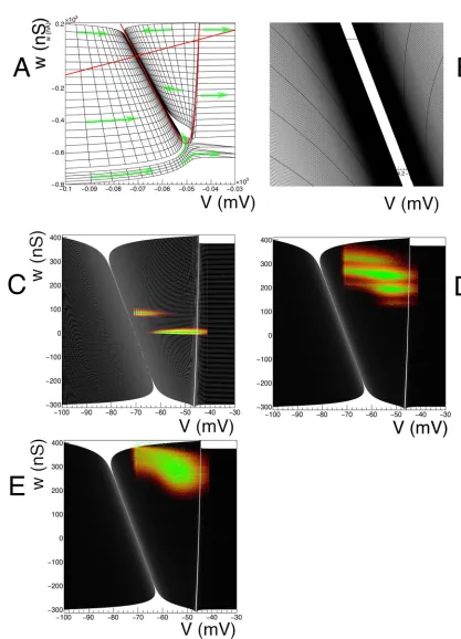
incoming spikes on the neurons. A conventional representation of such a model is given by a vector field, seeFig 1.
• A number of initial points are taken:
I¼ fV¼Vmin;i¼0;� � �ng;g¼iDgj ðV;gÞg;
for given fixedVmin,ng,Δg
Table 1. Constants taken from Apfaltrer et al. (2006), Appendix B.
membrane time constant τm 20 ms
reset potential Er -65 mV
reversal potential Erev -65 mV
equilibrium potentiale Ee 0 V
synaptic time constante τs 5 mV
threshold potential Vth -55 mV
Fig 1. A: Vector field for a conductance based model, along with a few integral curves. At very low conductance, there is a
Consider a two dimensional dynamical system defined by a vector field. A point in state space will be represented by a two dimensional vector~v. A grid is constructed from strips. As mentioned previously, usually one dimension is a membrane potential, and we will denote coordinates in this dimension by a small letterv. The second dimension can be used to repre-sent parameters such as adaptation, conductance, and will be reprerepre-sented byw. A strip is con-structed by choosing two neighbouring points in state space, e.g.v~0ðt¼0Þ; ~v1ðt¼0Þ, and
integrating the vector field for a timeTthat is assumed to be an integer multiple of a period of timeΔt, which we assume to be a defining characteristic of the grid. LetT=nΔt, then two dis-cretized neighbouring characteristics
S¼ fv~0ðt¼0Þ;� � �; ~v0ðt¼nDtÞ;v~1ðt¼0Þ;� � �; ~v1ðt¼nDtÞg
define a strip. Within a strip, the set of points
Ci ¼ f~v0ðt¼iDtÞ; ~v0ðt¼ ðiþ1ÞDtÞ; ~v1ðt¼ ðiþ1ÞDtÞ; ~v1ðt¼iDtÞg
defines a cell, which is quadrilateral in shape. The quadrilateral should besimple, but not nec-essarilyconvex(Fig 2A). We reject cells with less than a certain area. As we will see in concrete examples, boundaries in state space are approached through areas of vanishing measure. The area cut tends to remove complex cells, and we will reject them in general. An example of a grid generated by this procedure is given inFig 3.
Strip numbers are arbitrary, as long as they are unique, but it is convenient to number them in order of creation. In the remainder of the paper, we will assume that strip numbers created by the integration procedure start at 1, and are consecutive, so that the numbersi2{1,� � �,
Nstrip} withNstripthe number of strips, each identify a unique strip. Strip no. 0 is reserved for
stationary points. There may be 0 or more cells in strip 0. The number of cells in stripiis denoted byncell(i). We refer to the tuple (i,j), withithe strip number andjthe cell number, as
thecoordinatesof the bin in the grid.Ncellsis the total number of cells in the grid.
For all stripsi(i>0 by construction), cell numbers within a strip are ordered by the dynamics: neurons that are in cell numberjof stripiat timetare in cell numberj+ 1 modnj
of stripjat timet+Δt, wherenjis the number of cells in that strip.
Neurons that are in a cell in strip no. 0 are assumed to be stationary and do not move through the strip. Examples of cells in this strip are reversal bins. The handling of stationary bins will be discussed below.
Representing a density profile
A simulation progresses in multiple steps ofΔt, so the current simulation timetsimis specified
by an integerk, defined by:
tsim¼kDt; k¼0;1;2;� � �
The density profile can be represented in an arrayMof lengthNcells. Each element of this
array is associated with the grid as follows. Letccell(0)�0 and for 0<i�Nstripletccell(i)� ccell(i−1) +ncell(i−1), soccell(i) represents the total number of cells in all strips up to stripi.
numbers are arbitrary, as long as they are unique, but it is convenient to number them in order of creation. By construction, cell numbers within a strip are ordered by the dynamics: neurons that are in cell numberjof stripiat timetare in cell numberj+ 1 modnjof stripjat timet+Δt, wherenjis the number of cells in that strip.
Now define the index functionI:
i¼0 Iði;j;kÞ ¼j
i>0 Iði;j;kÞ ¼ccellði 1Þ þ ðj kÞmodncellðjÞ
(
ð9Þ
This is a time dependent mapping: its effect is a forward motion of probability mass with each forward time step. We will refer to the updating of the mapping by incrementingkas amass
[image:9.612.50.574.75.504.2]rotationas probability mass that reaches the end of a strip, will reappear at the beginning of
Fig 2. A: As a result of the integration procedure simple quadrilaterals (left, middle) should emerge, which are usually convex (left), except near stationary points or
limit cycles where concave quadrilaterals (middle) can be formed. Complex, i.e. self-intersecting, quadrilaterals can occur around strong non linearities, for example the crossing of nullclines. These definitions hold for any polygon. B: The problem of defining the Master equation: we can easily calculate how much mass per unit time leaves a given bin (i,j). This mass will reappear at a positionhaway from the original bin, wherehis the synaptic efficacy. In the figure bin (13,7) is translated along vector (0, 0.1). This corresponds to neurons that have received an input spike, and therefore are experiencing a jump in conductance. Most neurons that are in bin (13,7), will end up in bin (13, 5) and (14,4), with some in bin (13,6) and (14,6). SoC(0.,0.1)(13, 7) = {(13, 5), (14, 5), (13, 6), (14, 6)}. C: Some events will end up
outside of the grid after translation. D: Fiducial quadrilaterals can be used to test where they have gone missing, and where is the best place to reassign them to the grid.
the strip at the next time step. This effect is almost always undesirable as it would effect a jump wise displacement of probability mass. In most models this can be prevented by removing the probability mass from the beginning of each strip and setting the content of this bin to 0, and adding the removed mass to a another bin. A typical example arises in the case of integrate-and-fire models. Here, there is usually a reversal point. Such a point can be emulated by creat-ing a small quadrilateral, and makcreat-ing this cell number 0 in strip number 0.
[image:10.612.297.466.274.437.2]The procedure of mapping probability mass from the beginning of a strip to special bins in state space is called areversal mapping. It consists of a list of coordinate pairs. The first coordi-nate labels the bin where probability will be removed, the second coordicoordi-nate labels the bin where the probability will reappear. The concept of reversal mapping extends to other neural models—we will consider adaptive-exponential-integrate-and-fire (AdExp), Fitzhugh-Nagumo, and quadratic-integrate-and-fire neurons. All of these models need a prescription for what happens with the probability mass after reaching the end of a strip, and we will refer to this as the reversal mapping, even if the model does not really have a reversal bin, to contrast
Fig 3. Probability mass is maintained in a mass array. In general, mass does not move, except when the mass has
moved beyond the end of a strip. The relationship between the mass array and the mesh is updated with each time step, resulting in the apparent motion of probability mass through the mesh (top left and top right). At the end of each simulation step, probability mass is removed from each first bin of the strip, and added to a special quadrilateral (bottom): the reversal bin. Mass does not move from here, and only synaptic input can cause mass to leave this bin.
it from thethreshold mapping. Although handling a threshold is similar, interaction with syn-aptic input means that the mapping requires extra precautions. We will discuss this in the sec-tion below.
The whole process of advancing probability through a grid by means of updating a relation-ship with a grid is illustrated inFig 3. Up to this point we have only referred to probability mass. If a density representation is desired, one can calculate the density by:
rði;jÞ ¼Mði;j;kÞ
Aði;jÞ ; ð10Þ
whereAði;jÞis the area of quadrilateral (i,j), andMði;j;kÞis the probability mass present in the quadrilateral (i,j) at simulation timekΔt. We note that this procedure implements a com-plete numerical solution for the advective part ofEq 2.
Handling synaptic input
We will assume that individual neurons will receive Poisson spike trains with a known rate for a known synaptic distribution of the post synaptic population. Without loss of generality we will limit the exposition to a single fixed synaptic efficacy; continuous distributions can be sampled by generating several matrices, one for each synaptic efficacy, and adding them together. Adding the individual matrices, which are band matrices, and very sparse, results in another band matrix, still sparse, albeit with a slightly broader band. Overall run times are hardly affected unless really broad synaptic distributions are sampled.
A connection between two populations will be defined by the tuple (Ncon,h,τdelay). Here Nconis the number of connections from presynaptic neurons onto a representative neuron in
the receiving population,τdelaythe delay in the transmission of presynaptic spikes andhthe
synaptic efficacy. The firing rateνis either given, or inferred from the state of the presynaptic population, but in both cases assumed to be known. For the population these assumptions lead to a Master equation:
Z
V
d~vdrð~v;tÞ
dt ¼n
Z
Vh
d~v0rð~v0;tÞ Z
V
d~vrð~v;tÞ
� �
; ð11Þ
whereVis an area of state space andVhthe same area, translated by an amounthin dimension i. It is dependent on the neuronal model in which variable the jump takes place. In AdExp the jump is in membrane potential, in conductance based models it is in the conductance variable. Here, we will discuss the problem using conductance based neurons as an example, but the methodology applies to any model.
Eq (11)determines the right hand side ofEq (2), and the stage is set for numerical solution. The left hand side ofEq (2)describes the advective part, and is purely determined by the neu-ron model, which ultimately determines the grid. We already have described the movement of probability mass due to advection during a time stepΔt, and need to complete this by imple-menting a numerical solution forEq (11).
Eq (11)describes the transfer of probability mass from one region of state space to another. We will assume that the grid we use for the model of advection is sufficiently fine, so that the density within a single bin can be considered to be constant, and choose areaVinEq (11)to coincide with our grid bins. We approximate (11) by:
dMði;j;kÞ
dt ¼n
X
ðp;qÞ2Chði;jÞ
ap;qMðp;q;kÞ Mði;j;kÞ
( )
The bin (i,j) translated by a distancehwill cover a number of other bins of the grid. Let (p,q) be a bin partly covered by the translated bin (i,j) and letαp,qbe the fraction of the surface area
of the translated bin that covers bin (p,q). (By construction 0<αp,q�1.) The setCh(i,j) is
defined as the set of tuples (p,q), for all such bins, i.e. those bins that are covered by translated bin (i,j) (and no others). We will refer toCh(i,j) as thedisplacement set. Usually, the
displace-ment is in one dimension only, where this is not the case we will writeC~hði;jÞ. The problem of determiningCh(i,j) is one of computational geometry that can be solved before simulation
starts. It is illustrated inFig 2B, where the grid of the conductance based model is shown. This problem is easily stated but hard to solve efficiently. Conceptually, a Monte Carlo approach is simplest, and since the computation can be done offline—before simulation starts—this approach is preferable. It is straightforward for a given bin of the grid (i,j) to gen-erate random points that are contained within its quadrilateral. Assume these points are trans-lated by a vector~h. It is now a matter of determining in which bin a translated point falls. In order to achieve this the grid is stored as a list of cells. Each cell, being a quadrilateral, is repre-sented by a list of four coordinates. During construction of the grid, vertices of a cell are stored in counter clockwise order.
When a quadrilateral is convex, and the vertices are stored in counter clockwise order, the×operator defined by:
� v1
v2 !
� v2
v1 !
results in an “inward” pointing normal~n. If the position vector of a point has a positive scalar product with the ‘inward’ normal of all four line segments that define the quadrilateral the point is inside, otherwise it is outside. These half line tests are cheap and easy to implement. If the quadrilateral is not convex, but simple, it can be split into two triangles which are convex.
We perform linear search to find a grid cell that contains the translated point, or to con-clude there is no such cell. Better efficiency can be obtained with k-d trees, but we have found the generation of translation matrices not to be a bottleneck in our workflow, and linear search allows straightforward brute force parallelization. At most one cell will contain the translated point. For now, we will assume that the translated point will be inside a given bin (p,q). Later, for concrete neuron models we will discuss specific ways of handling transitions falling outside the grid. If bin (p,q) is not represented inC~hði;jÞ, an entry for it will be added to it. The process is then repeated, in totalNpointtimes. For each cell (p,q) represented inCh~ði;jÞa countn(p,q)is
maintained andαp,qis estimated by:
ap;q¼ nðp;qÞ
Npoint
ð13Þ
Eq 12is of the form
dM
dt ¼T �M;
whereT is called the transition matrix. The displacement set determines the transition matrix. Here, we have described a Monte Carlo strategy that uses serial search to determine the set
C~hði;jÞand consequently the constantsαp,qfor bins (p,q) in that set. With these constants
determined, it is a straightforward matter to solveEq 12numerically.
The main algorithm now consists of three steps: updating the index relationshipEq 9, which constitutes the movement of probability mass through the grid during a time interval
matters. Implementing the reversal bin after the master equation may lead to removing proba-bility mass from the beginning of the strip that should have been mapped to a reversal bin.
Handling a threshold
Many neuron models incorporate a threshold of some sort. For example, in the original con-ductance based model by [20], a threshold of -55 mV is applied. This corresponds to a vertical boundary in the (V,g) plane (seeFig 1). Neurons that hit this threshold from lower potentials generate a spike and are taken out of the system. After a periodτref, they are reintroduced at
(Vreset,g(tspike+τref)), wheretspikeis the time when the neuron hits the threshold, andg(tspike)
is the conductance value the neuron had at the time of hitting the threshold. In this model, fol-lowing [20], it is assumed that the conductance variable continues to evolve according toEq 8, without being affected by the spike.
We handle this as follows. For each strip it is determined which cells contain the threshold boundary, i.e. at least one vertex lies below the threshold potential and at least one lies on or above the threshold potential. The set of all such cells is called thethreshold set. In a similar way aresetset is constructed, the set of cells that contain the reset potential. In the simplest case, for each cell in the threshold set the cell in the reset set is identified that is closest inwto that of a threshold cell. The threshold cell is then mapped to the corresponding reset cell and the set of all such mappings is called the reset mapping.
Sometimes, the value ofwis adapted after a neuron spikes. In the AdExp model, for exam-ple,w!w+bafter a spike. In this case, we translate each cell in the reset set in direction (0,
w), and calculate its displacement set, just as we did for the transition matrix. The reset map-ping is then not implemented between the threshold cell and the original reset cell, but to the displacement set of that reset cell. We do this for all threshold cells and thus arrive at a slightly more complex reset mapping.
Due to the irregularity of the grid, it may happen that some transitions of the Master equa-tion are into cells that are above the threshold potential. This will lead to stray probability above threshold, if not corrected. We correct for this during the generation of the transition matrix. If during event generation a point ends up above threshold after translation, we look for the closest threshold cell for this point. The event is then attributed to that threshold cell, and not the stray cell above threshold. In this way transitions from below or on threshold to cells above threshold are explicitly ruled out.
The reset mapping must be carried out immediately after the solution of the master equa-tion, before the next update of the index function.
Gaps in state space
All grids are finite. For that reason alone the Monte Carlo procedure described above will result in translated points that cannot be attributed to any cell. Those events are lost and will lead to unbalanced transitions: mass will flow out of bins near the edge, but will not reappear anywhere else in the system and there is a possibility that mass evaporates from the system. This problem does not occur just at the edges, but also in the vicinity of stationary points. We will see that some dynamical systems display strong non linearities that will make it impossible to cover state space densely. The ability to deal with such gaps in state space is the most impor-tant technical challenge for this method.
straightforward to maintain a list of grid cells that have at least one vertex in the fiducial bin. We assign the event to the grid cell that is closest along the projection in the jump direction.
Fig 2Dshows the total number of events lost in the generation of transition matrix corre-sponding to a jump of 5 mV, thereby revealing gaps in state space. The orange quadrilaterals are the fiducial bins. After reassignments all events fall inside the grid and probability will be balanced.
Marginal distributions
It is straightforward to calculate marginal distributions. Again, we use Monte Carlo simulation to generate points inside a given quadrilateral (p,q). We then histogram these points invand
w. For each biniin thevhistogram, we can now estimate a matrix elementα(p,q),iby dividing
the number of points in biniby the total number of points that were generated. For a given distribution, one can now multiply the total mass in bin (p,q) byα(p,q),ito find how much of
this mass should be allocated to bini. If one does this for every cell (p,q) in the grid, one will find the distribution of mass over the marginal histogram, and can calculate the marginal den-sity from this.
Results/Discussion
We present a succession of population simulations of four neuronal models. A neuron with a single excitatory conductance has a simple state space, and its simulation provides few prob-lems. It is a familiar model and therefore a good one to introduce and demonstrate the formal-ism. We then move to one dimensional results and replicate some familiar results for LIF and QIF neurons: density profiles, transient firing rates and gain curves. This allows us to quantita-tively examine some of the strengths and weaknesses of the method. We then discuss two mod-els that show a progression of difficulty in covering state space: AdExp and Fitzhugh-Nagumo. Although a methods paper, we feel that nonetheless we can infer a number of general princi-ples that run as a common thread through our use cases, and we present them here.
• We obtain a general method for simulating populations of spiking point model neurons with a one or two dimensional state space, subject to Poisson spike trains. When restricted to one dimension, the method is equivalent to that published by de Kamps (2013) and Iyer
et al. (2013) and is very efficient, as the work of Cainet al. demonstrates. The method is able to replicate earlier work on 2D models, but is more general, as first, it is able to accept novel models in the form of a grid file and therefore does not require source code changes when a new model is considered, and second, does not rely on the diffusion approximation, but allows a variety of stochastic processes to be considered. The method is most efficient for synaptic efficacies and firing rates commensurate with what is found in the brain, but can be pushed to reproduce diffusion results, although dedicated numerical strategies for solving the ensuing 2D Fokker-Planck equations will be more efficient. Nonetheless, the possibility to study the diffusion limit as a special case is a useful property of the method.
• The method is insensitive to the gradient density, and will accurately model delta synapses and handle discontinuities of the density profile, and is able to model populations that are in partial synchrony, allowing the modelling of the decorrelation process itself.
the nullclines the system approaches a stable equilibrium or a limit cycle. The system does not contain enough information in one of the two dimensions and the grid cannot be mean-ingfully continued. We find that the motion of probability mass inside such a region can be inferred from the dynamics around it. A limit cycle, for example can be inferred from the grid closing onto it, even when we cannot extrapolate the grid directly to the limit cycle. In a similar way we can capture the motion of mass towards a stable equilibrium: when motion has stopped in one direction, but still continues in the other, we find that placing neurons that are deposited into accessible regions by synaptic input in nearby parts of state space accurately captures the overall motion of mass around these regions. Similar considerations apply around unstable regions of state space, and because we can time invert the dynamical system when constructing the grid, we find that these problems can be handled in much the same way.
• Transient responses can be understood in geometrical terms. If a boundary, either a reflect-ing or an absorbreflect-ing one, is present in state space, the population will exhibit a strong oscil-latory response (“ringing”) when the input is strong enough to push neurons towards the boundary and noise is too weak to disperse neurons before reaching it. The converse is also true: if despite the presence of a boundary, state space allows neurons a way around it, strong transients will be absent. Rate based models based on first order differential equations on using a gain function will model these transients incorrectly, or not at all.
• The method can describe the version of Tsodyks-Makram synapses used by Vasilaki and Giugliano [24] in a model of network formation.
• By far the most challenging grid to make was that of a Fitzhugh-Nagumo neuron, because the approach to the limit cycle in part also implies an approach to the nullcines of the system, leading to a loss of information in one dimension. Where the nullclines cross this problem is exacerbated. We find that we have to imply the limit cycle: we define the grid in the approach to the limit cycle and infer the deterministic dynamics in an area around the limit cycle from the surrounding grid cells.
Conductance based neurons
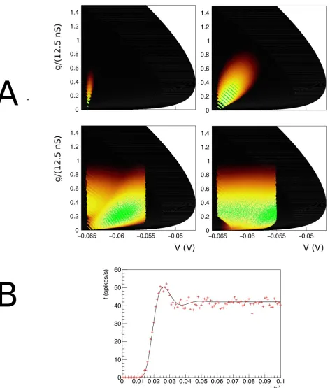
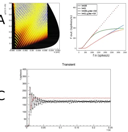
Fig 4. A: The evolution of the joint probability density function at four different points in time (1, 5, 15, 28 ms) in (V,g) space (Vmembrane potential,gconductance) for synaptic efficacyJ= 0.05, Poisson generated input spike train with rateν= 1000 spikes per second. B: The resulting population firing rate, calculated from the fraction of mass crossing threshold per unit time as a solid black line. Spiking neuron simulation results shown by red markers. Onset and resulting firing rates are in agreement throughout. Unlike one dimensional neural models, conductance based models produce almost no overshoot.
state at a given time as points in state space. The cloud of points clearly tracks the white areas of the density. The shot noise structure is clearly visible in the band structure early in the simu-lation where neurons are present at multiples of the synaptic efficacy, reflecting that some neu-rons have sustained multiple hits by incoming spike trains.
As neurons are moving through threshold, they themselves emit a spike and contribute to the response firing rate of the population, defined as the fraction of the population that spikes per time interval, divided by that time interval. We can therefore calculate the response firing rate from the amount of mass moving through threshold per unit time. We show the jump response of the population as a plot of populating firing rate as a function of time inFig 4B. The firing rate calculated from the density matches that calculated from the Monte Carlo sim-ulation very well. Interestingly, there is almost no overshoot in the firing rate, as also noted by Richardson (2004), who studied this system using Fokker-Planck equations. Although we study shot noise, in the absence of a fundamental scale in thegdirection, the central limit theo-rem ensures that the marginal distribution ingis Gaussian within a few milliseconds. It is clear that the population disperse in thegdirection and drifts towards the threshold relatively slowly. The absence of a barrier allows the dispersal of the population before it hits threshold, greatly reducing any overshoot in the firing rate, which is quite unlike one dimensional neural models, as we shall see in Sec. Results: One Dimension.
Let us contrast this with a simulation where we introduce a maximum conductancegmax=
0.8, which for simplicity we assume to be voltage independent. This then introduces a reflect-ing boundary atg=gmax, and therefore introduces a scale by which an efficacy can judged to
be small or large. As expected, probability mass is squashed against this boundary (Fig 5A) and has nowhere to go but laterally, in the direction of the threshold. Interestingly, the mass has not dispersed and clear groupings of mass huddled against the boundary can be observed. The traversal of the threshold by these groupings produces clear oscillations in the firing rate: a “ringing” effect. The firing rate jump response reflects the effect of the presence of a maximum conductance in state space.
We run two simulations: one with and one without maximum conductance, but otherwise identical, and repeat this experiment for two different synaptic efficacies:J= 1 and 3 mV. Both simulations use an input rate of 3 kHz. In the case of no maximum conductance, proba-bility mass can disperse in thegdirection and mostly does so before arriving at the threshold. InFig 5one sees that the introduction of a maximum conductance leads to a reduced response firing rate for high inputs. This can be interpreted as the population unable to respond to an increase of input once the majority of its ion channels are already open.Fig 5
shows that the firing rates of Monte Carlo simulations and our method agree over the entire range of input.
Even when the effects on the response firing rate are moderate, the transient dynamics can be radically different. For an efficacyJ= 1 mV and and input rateνin= 3 kHz, the firing
One dimension: Leaky- and quadratic-integrate-and-fire neurons and size
effects on the transition matrix
[image:18.612.73.508.71.520.2]Although these model neurons are characterized by a single dimension—the membrane potential—they can be viewed as a two dimensional model that is realized in a single strip, and where transitions take place between one bin in potential space to another. This is completely equivalent—in implementation and concept—to the geometric binning method introduced independently by de Kamps [12] and Iyeret al. [11], with one exception: the generation of transition matrices by Monte Carlo. In one dimension it is not necessary to use Monte Carlo
Fig 5. A: The density att= 15 ms. Events are reflected against a reflecting conductance boundary. B: Gain curves for different input rates and synaptic efficacies. The maximum conductance clearly affects the shape of the gain curves, although at input rate 3 kHz forJ= 1 mV the effect is moderate. C: The transient looks very different in the case where a maximum conductance is present (red): the “ringing effect” is much stronger, compared to the case without maximum (black), while the overall firing rates do not differ greatly. The cause can be seen in A: neurons have not had time to disperse before they are forced across threshold; clear groupings can be seen at the maximum conductance.
generation: the transition matrix elements can be calculated to an arbitrary precision because in one dimension the geometrical problem outlined in Sec. Materials and Methods: Handling Synaptic Input is much simpler and can be solved by linear search. It is clear that unlike the 2D case, it is straightforward to find the exact areas covered by translated bins, and hence no Monte Carlo generation process is required.
Nevertheless, it is interesting to use this method. The transition matrix generation for the 2D case is relatively expensive, and as precision scales with the square root of the number of events it is interesting to see how few we can use in practice without distorting our results. The answer is: surprisingly few. As benchmark we set up a population of LIF neurons with mem-brane constantτ= 50 ms, following [5], and assume that each neuron receives Poisson distrib-uted spike trains with a rateν= 800 Hz. We assume delta synapses, i.e. an instantaneous jump in the postsynaptic potential by a magnitudeh= 0.03, with the membrane potentialV2[−1, 1), i.e. we use a rescaled threshold potentialV= 1. The grid is generated with a time step
Δt= 0.1 ms, and is shown inFig 6B.
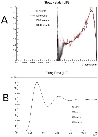
The simulation results are shown inFig 7and replicates earlier work [5,12]. The use of a finite number of points in the Monte Carlo process used for the generation of transition matrices generates random fluctuations with respect to the true values. The effect of these fluctuations is clearly visible in the shape of the density profile, and only forNpoint= 10000
the profile is as smooth as in earlier results where we calculated the transition matrix analyti-cally. How bad is this? To put these fluctuations into perspective, we used a direct simulation of 10000 spiking neurons and histogrammed their membrane potential at a simulation time well aftert= 0.3 s, so that they can be assumed to sample the steady state distribution. In the figure, they have been indicated by red markers. Comparing the results we see that the fluctu-ations forNpoint= 10 are comparable to those of a Monte Carlo simulation using a sizeable
population of 10000 neurons. Moreover, in the population firing rates the finite size effects are almost invisible. This is somewhat surprising, but a consideration of the underlying pro-cess that generates the firing rate explains this. Neurons are introduced at equilibrium and will undergo several jumps before they reach threshold. The finite size effects of the Monte Carlo process induce variations in those jumps in different regions of state space, but these fluctuations are unbiased and will average out over a number of jumps. So neurons will expe-rience variability in the time they reach threshold, but this variability does not come in the main from fluctuations in the transition matrix elements. It should be emphasized that the transition matrices are a quenched source of randomness, because transition matrices are fixed before the simulation starts. So although ultimately caused by finite size effects, their contribution is different compared to the unquenched finite size effects that can be seen in the population of 10000 neurons.
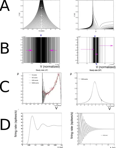
It is instructive to look at some examples because it highlights strengths and weaknesses of the method in terms of familiar results. InFig 6A, the characteristics of both neural models are given. InFig 6Bthe state space of LIF (left) and QIF neurons (right) are shown, at lower resolu-tion than used in simularesolu-tion to elucidate the dynamics. Rather than with numbers which would be unreadable at this scale, we indicate the direction in which cell numbers increase, and therefore the direction in which neural mass will move, by arrows. One can see that the LIF neuron is comprised of two strips, and the QIF neuron of three, where the arrows indicate in which direction the cell numbers are increasing. In the LIF grid, there is one stationary bin, in the QIF there are two. They are represented as separate stationary cells, covering the space between the strips, indicated by the blue downward pointing arrows.
InFig 6Cwe consider the steady state of LIF (left) and QIF neurons (right) after being sub-jected to a jump response of Poisson distributed spike trains starting att= 0 (LIF:νin= 800
and therefore of the grid clearly reflect their influence on the steady state density distribution. The output firing rate (Fig 6D) shows the clear “ringing” in the transient firing rate that is mostly absent in conductance based neurons. Again, this can be interpreted geometrically: the stochastic process pushes neurons in the direction of a threshold, but they reach it without having had the opportunity to disperse. Decorrelation only happens after most neurons have
Fig 6. A: Characteristics for leaky- (left) and quadratic-integrate-and-fire (right) neurons. B: The resulting grids for both
neuron types. C: Typical steady state densities, strongly influenced by the shape of the grid, and ultimately the neural dynamics. D: a typical jump response of the firing rate. For comparable output frequencies, QIF neurons “ring” for longer, which we attribute to a closer grouping of probability mass.
Fig 7. A: The steady state density as a function of membrane potential. B: The firing rate as a function of time, for transition
matrices that were generated for different values ofNpoint, the number of events used in the Monte Carlo generation of
transition matrices.
gone through threshold at least once. It is also interesting to see that for comparable firing rates the ringing is much stronger for QIF than for LIF neurons. We also interpret this as a geometrical effect: the effective threshold for QIF neurons isV= 3 (normalized units), not 10, as neurons with a membrane potential above 3 will spike. It is clear fromFig 6Dthat compared to LIF neurons, QIF neuron bulk up close to the threshold and are constrained more than their LIF counterparts, thereby making it harder to decorrelate before passing threshold.
For reference, inFig 8we show that the method accurately reproduces results from the dif-fusion limit, as well as generalizes correctly beyond it. If one uses a single Poisson spike train to emulate a Gaussian white noise input, employing the relationship:
m ¼ninJt
s2 ¼n
inJ
2t; ð14Þ
one can use our method to predict the steady state firing rates as a function ofJ, the synaptic efficacy andνinthe rate of the Poisson process for given membrane constantτ. Organizing the
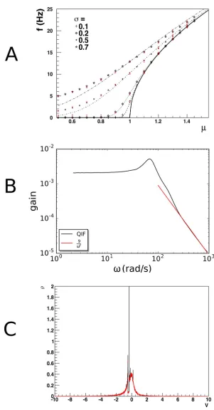
results in terms ofμandσ, as given byEq 14, one expects a close correspondence for lowσ, sinceEq 14leads to small values ofJcompared to threshold. One expects deviations at highσ, whereJdoes not come out small.Fig 8shows that this is indeed the case when firing rates are compared to analytic results obtained in the diffusion approximation. Our method produces the correct deviations from the diffusion approximation results, and agrees with Monte Carlo simulation. Elsewhere [12], we have shown that diffusion results can be accurately modeled using two Poisson rates for highσ.
InFig 8Bwe replicate the gain spectrum for QIF neurons and show that the high frequency dependence falls off as 1
o2as predicted by Fourcaud-Trocme´et al. [25]. These results reaffirm that our method accurately predicts results within and beyond the diffusion limit, and that a substantial body of existing literature can be seen to be a special case of our method.
Fig 8Cshows a population of QIF neurons that fire in synchrony att= 0, undergoing a slow decorrelation by low rate Poisson input spike trains. The neurons have all been prepared in the same state, and therefore are at the same position in state space. We useF(V) =V2+ 1, so these neurons are bursting, as the current parameter is larger than 0, and there are no fixed points. Neurons that receive an input spike leave the peak and travel on their own through state space. This results in a very complex density profile, where the initial density peak is still visible after 1s. Such a peak would have diffused away rapidly in a diffusion limit approxima-tion. Monte Carlo events in red markers show that the density profile is not a numerical arte-fact, but reflects the complexity of the density profile.
Adaptive-exponential-integrate-and-fire neurons
We consider the AdExp model as presented by Brette and Gerstner [26], which describes indi-vidual neurons by the following equations:
Cm
dV
dt ¼ glðV ElÞ þglDTe
ðV VTÞ
DT wþI
twdw
dt ¼aðV ElÞ w
ð15Þ
Upon spiking, the neuron is reset to potentialVresetand increases its adaptivity value:w!w+
b. HereCmis the membrane capacity andglthe passive conductance.VTis the value at which a
neuron starts to spike; the spike dynamics is controlled byΔT. The numerical values of the
Fig 8. A: Gain curve for quadratic-integrate-and-fire neurons. Population density techniques handle deviations from
the diffusion approximation correctly: when one tries to emulate Gaussian white noise with a single Poisson spike train input, deviations are expected at high values ofσas synaptic efficacies are forced to be large. The dashed lines give the diffusion approximation, black markers the prediction by our method and red bars Monte Carlo results, which agree with each other, but deviate from the diffusion prediction. B: The frequency spectrum shows the expected1
o2
An overview of the state space is given inFig 9A. Atw= 0 the dynamics is as expected, a drive towards the equilibrium potential that suddenly reverses into a spike onset at higher val-ues ofV, essentially producing an exponential-integrate-and-fire neuron. At highwtwo effects conspire to make the neuron less excitable: the equilibrium potential is lower and the drive towards this equilibrium is stronger for a given value ofV. At lowwvalues, the opposite hap-pens: the equilibrium value is higher, closer to threshold, and below equilibrium there is a stronger depolarizing trend making the neuron more excitable. Interestingly, at hyperpolariza-tion the system does not only respond by driving the membrane potential back towards equi-librium potential, but also downwards.
There are two critical points, the equilibrium point (El, 0) and a saddle point in the top
right. They are at the crossing of two nullclines: thew-nullcline is a straight line, whereas the
V-nullcline follows a strongly curved trajectory, which is close to the stable manifold of the saddle point in a substantial part of state space. Below (to the right) the stable manifold neu-rons spike, regardless of where they are initially, while above (to the left) of the stable manifold neurons converge to the equilibrium, but how, and how long this takes is strongly dependent on the initial conditions. This model is the first to require a judicial treatment of the grid boundaries.
Let us examine the the equilibrium point first. The exponential build-up of cells observed in one dimensional models occurs here as well, but here it is not a good idea to introduce a fidu-cial cut and cover the remaining part of state space with a cell. The inset ofFig 9Bshows that equilibrium is reached much faster in theVdirection, than in thewdirection. This is a direct consequence of the adaptation time constantτwbeing an order of magnitude larger than the
membrane time constantτ�Cm/gl. For highw, mass will move downwards along the
[image:24.612.200.575.89.205.2]diago-nal, until low values ofware reached, as is demonstrated by the left inset ofFig 9. A long, but very narrow region separates different parts of the grid. What to do? First, we observe that the offending region is essentially forbidden for neurons: for most neurons starting from a ran-dom position in state space it would take a long time (of the order of 100 ms) to approach this no man’s land. At the input firing rates we will be considering, neurons will experience an input spike well before running off the strip, so essentially only noise can place neurons there. If we forbid this, by allocating events that are translated into the cleft between the two grid parts to the cells in the grid that are closest to it along the projection of the jump, we guarantee that no probability mass will leak out of the grid. Mass that reaches the end of the strips will be placed in a reversal bin, like the one dimensional case. Mass on the left of the side of the cleft will move in the same direction as that on the right side of the cleft. By using Euclidean dis-tance projected along the jump direction, we minimize the bias due to this procedure, although we may artificially introduce a small extra source of variability.
Table 2. Parameters for the AdExp model as given in [26].
Quantity Value
Cm 281 pF
gl 30 nS
El -70.6 mV
VT -50.4 mV
ΔT 2 mV
τw 144 ms
a 4 nS
b 0.0805 nA
Fig 9. A: Overview of state space for the adaptive-exponential-integrate-and-fire neuron. B: a detail of a realistic mesh near the
equilibrium potential. C-E: evolution of the probability density att= 0.01, 0.1, 0.4s. The input (switched on att= 0) is a Poisson distributed spike train of 3000 spikes/s, delta synapses with efficacyJ= 1 mV.
On the right hand side, the stable manifold almost coincides with theVnullcline, resulting in a very narrow region of dynamics in the vertical direction. Immediately outside neurons rapidly move away laterally. This part of the grid is created by reversing the time direction, integrating towards the stable manifold. The grid strongly deforms here: cell area decreases rapidly and even small numerical inaccuracies will lead to cells that are degenerate. We use cell area as a stopping criterion. The last cells before breaking off are extremely elongated. The spike region is also created by reversing the time direction. Again, we conclude that the cleft is a forbidden area: a small fluctuation in the state variable will cause a neuron to move away rap-idly. Our main concern, again, is neurons that are placed into this cleft by the noise process. Again, we move neurons to the closest cell next to the cleft in the jump direction. This is rea-sonable, since natural fluctuations would put them there soon anyway. Effectively we have broadened the separatrix a little bit, but we still capture the upwards (for highw—past the sad-dle point: downwards) movement close to the stable manifold.
InFig 9C–9Ethe evolution of a population in (V,w) space is shown at three different points in time:t= 0.05, 0.1 and 0.4 s.Fig 9Cshows the input spikes pushing the state towards thresh-old, and a small number of neurons have spiked. They re-emerge at the reset potential, but with much higherw, due to spike adaptation. This is determined by thebparameter of the AdExp model. Close to the reset potential the banded shot noise structure, due to the use of a delta-peaked synaptic efficacy, is visible. The steady state is reached after approximately 400 ms. The population stabilizes at highwvalues, and the bulk of the population is clearly well below threshold, due to stronger leak behavior at these values ofw. In sub figure E there is a minute deformation of the density, due to the limits of the grid, and density heaps up here, but the fraction of probability mass affected is negligible. Monte Carlo events, indicated by the dots, are not restricted to the grid and some fall outside the grid.
The firing rate response corresponding to the population experiencing an excitatory input (Fig 9C–9E) is given inFig 10A. Again, agreement with Monte Carlo simulation is excellent, we are able to study the relative contributions of current- and spike-based adaptation to the firing rate. We can easily simulate neurons with current- but not spike-based adaptation by not incor-porating the jump inwafter reset; while ignoring all forms of adaptation can be done by simply using a 1D grid and ignoring values ofw6¼0. The vast difference between adaptive neurons and non-adaptive neurons is also reflected in the gain spectrum.Fig 10Bshows the gain spectrum of a (non-adaptive) exponential-integrate-and-fire neuron and a neuron that has a constant rate of adaptation due to the background rate upon which the small sinusoidal modulation has been imposed. The difference between the adaptive and non-adaptive neuron is considerable. Both neurons show a1
odependence in the high frequency limit, as is expected for exponential neurons
[25]. (Fig 10Ashows that the shape of the spike, which is reflected in the large cells on the right of the grid is independent ofw.) It is clear that a meaningful time-independent gain function cannot be chosen, so that it is not possible to develop linear response theory.
It is interesting to observe the marginal distributions—inFig 11we show the marginal dis-tributions, together with the joint distribution. The distribution inVlooks remarkably like that of an LIF neuron, except near the threshold, where the spike region, which is not present for LIF, flattens the density. Thewdistribution suggests a much stronger overlap than the joint distribution, which shows a clear separation. It is clear that, had the three density blobs been oriented more diagonally, the marginalwdistribution would have shown a single cluster.
Frequency-dependent short-term synaptic dynamics
Fig 10. A: compares the response for three cases: no adaptation; only current adaptation; and both current- as well as
spike-based adaptation is included. B: The gain for a small sinusoidal input modulated on a background input as function of frequency, for no adaptation and AdExp with current- and spike-based adaptation. Both spectra show the1
odependency expected of an
exponential-integrate-and-fire neuron, as the spike shape, represented by the grid at highVvalues is independent ofw. However, the numerical difference between the cases is vast.
simulations they considered both spike-timing dependent long-term plasticity, and frequency-dependent short-term dynamics, where they use a version of the Tsodyks-Markram synapse [27]. The short-term dynamics is of interest because it introduces something we have not con-sidered before: the magnitude of the jump being dependent on the position of where the jump originates. Following [24], ifGijdefines the amplitude of the postsynaptic contribution from
Fig 11. Comparison of the joint distribution function of the AdExp neuron with the marginals inVandw. The marginalwdistribution still reveals four clusters, but the joint distribution reveals them as being far better resolved than one would judge from the marginals.
presynaptic neuronjto postsynaptic neuroni, then this is considered to be proportional to the amount of resources used for neurontransmissionuijrijand to their maximal availabilityAij, so
Gij¼Aijuijrij; ð16Þ
whererrelates to the recovery anduto the facilitation of synapses, and the time constantsτrec
andτfacilare different for facilitating and depressing synapses. They describe
frequency-depen-dent short-term synaptic dynamics by:
drij
dt ¼ ð1 rijÞ=trec uijrij
X1
kj
dðt tkjÞ ð17Þ
duij
dt ¼ uij=tfacilþUð1 uijÞ
X1
kj
dðt tk
jÞ ð18Þ
From now on, we will drop the indicesijand just refer to a single connection. In the simula-tion below we will useτrec= 0.1 s andτfacil= 0.9 s and study a population of facilitating
synap-ses (Vasilaki and Giugliano usedτrec= 0.9s,τfacil= 0.1 s for depressing synapses.)Uis a fixed
constant, for facilitating (depressing) synapsesU= 0.1(0.8).Eq 17expresses that an individual synapse is subject to deterministic dynamics, and that upon the arrival of a spike at timetk
bothuandrundergo a finite jump, whose magnitude is dependent on the current value ofu
andr.Eq 2describes this situation, when the following transition probabilities are introduced:
Wðr0;u0jr;uÞ ¼ndðr0 rþurÞdðu0 u Uð1 uÞÞ ndðr0 rÞdðu0 uÞ ð19Þ
We have to modify the process of generating our transition matrices: now for each quadrilat-eral cell (p,q), we determine the centroid (u(p,q),r(p,q)) and we determine the covering set by
defining
~h¼ uðp;qÞrðp;qÞ Uð1 uðp;qÞÞ 0
@
1
A ð20Þ
and determining the cover set as before. The jump now becomes cell dependent.
It is easy to cover almost the entire state space. InFig 12Awe show the grid. InFig 12B, we show the sample path of three synapses, assuming that the presynaptic firing rateν= 5 Hz. In C-F we show the evolution of a population of synapses. The influence of the step size which increases in ther(horizontal) direction withuandr, but decreases in theu(vertical) direction withu. There is good agreement with Monte Carlo simulation throughout. With the joint dis-tribution available, it is possible to useEq 16and calculate the distribution ofGijor its
expecta-tion value.
Fitzhugh-Nagumo neurons
We consider the well-known Fitzhugh-Nagumo neuron model [28], which is given by:
dV
dt ¼V
V3
3 WþI
dW
dt ¼0:08ðVþ0:7 0:8WÞ

![Table 2. Parameters for the AdExp model as given in [26].](https://thumb-us.123doks.com/thumbv2/123dok_us/1827380.138584/24.612.200.575.89.205/table-parameters-adexp-model-given.webp)