Robotic manipulation for granular materials

(1)

R o b o tic M a n ip u la tio n fo r

G r a n u la r M a te r ia ls

Kegen Yu

B.Sc. Changchun (China)

Graduate Diploma

Shandong (China)

October 1998

A thesis submitted for the degree of M aster of Engineering

of The Australian National University

Department of Engineering

(2)

D e c la r a tio n

T his thesis contains no m aterial which has been previously accepted for th e aw ard of any o th er degree or diplom a a t any university, in stitu te or college, an d contains no m aterial previously published or w ritte n by an o th er person, except where due reference

is m ade.

C an b erra, O ctober 1998.

C o n fe r e n c e P ap er:

[Cl] Kegen Yu an d Jo n Kieffer, ” R obotic force/velocity control for following unknow n contours of g ranular m aterials,” su b m itte d to th e 1999 IE E E In te rn atio n a l Conference on R obotics and A u to m atio n (D etro it, M ichigan, USA, May 1999).

[C2] Kegen Yu and Jo n Kieffer, ” R obotic force control for following unknow n contours

of gran ular m aterials,” Proceedings o f the IA S T E D Intern atio na l Conference on Control

and A pplications, Honolulu, Hawaii, USA, A ugust 12-14, 1998.

[C3] Jo n Kieffer, Kegen Yu, Junm ei Cao and K. Maw, “Toward blind grouping: an

approach to m an ip u latio n in unknow n sensor-hostile environm ents,” Proceedings o f the

Kegen Yu D ep artm en t of E ngineering Faculty of Engineering and Inform ation Technology T he A u stralian N ational U niversity C a n b e rra A C T 0200, AU STRA LIA .

(3)

International Conference on Field and Service Robotics, pp.449-455, Canberra, Decem

(4)

A b s t r a c t

In th is thesis, we deal w ith th re e m ain problem s: proposing and verifying a m odel ch aracterising force interactions betw een th e spherical tool and th e pile of gran ular m aterials; developing a control algorithm to realize tool m ovem ent over th e contour of th e pile of gravel; and proposing an indirect adaptive control to tackle th e u n certain ties in th e m odel p aram eters.

By analysing th e experim ental d a ta obtained by lettin g th e tool push th e pile w ith shallow d e p th , we propose an interaction m odel s tru c tu re . T his ap p rox im ate m odel s tru c tu re is quite sim ple since it has only two p aram eters. By use of least-square identification m eth o d , we get th e estim ate of these two p aram eters. T his m odel can be used to estim ate th e contact d e p th and th e surface norm al online. T he experim ental results d em o n strate th a t the estim ated d e p th and surface norm al are reliable.

T h en we develop a contour following algorithm which uses force feedback to a d ju s t th e desired norm al force. B oth force m easurem ents and position inform ation are utilised to estim ate th e surface norm al and tan g en tial online. A velocity-based position control system is used to move th e tool along different plan ar contour shapes w hen th e m odel p a ra m ete rs are known. M any sim ulations and experim ents are done w ith various controller p a ram eters and m odel p aram eters. T he sim ulation and experim ental resu lts using SCARA ro b ot illu strate th e effectiveness of th e proposed control algorithm .

Finally, considering th e u ncertain ties in th e m odel p aram eters, we in trod uce an indirect a d a p ta tio n m echanism into th e control algorithm . T he m odel p a ra m ete rs are e stim a ted explicitly on line. Sim ulation and experim ental results d em o n strate th a t th e proposed ad aptiv e m eth o d is feasible.

(5)

A c k n o w le d g e m e n ts

I would like to thank my supervisor, Jon Kieffer, for all of his efforts, encouragement,

support and his appointing me as his teaching assistant over the last year. I would also

like to thank M att James who appointed me as his teaching assistant. And I would like

to thank all of the people in the Department of Engineering who helped me and made

it possible for me to complete my thesis in one year. Finally, I would like to thank my

family so much who have given me in terms of education, encouragement, moral and

financial support.

(6)

C o n te n ts

D e c la r a tio n i

A b s t r a c t iii

A c k n o w le d g e m e n ts iv

N o t a t io n x iii

A b b r e v ia t io n s x v

1 I n t r o d u c tio n 1

1.1 B ack g ro u n d ... 1

1.2 Organisation of this Thesis ... 2

2 A M o d e l for I n te r a c tio n w it h G ra n u la r M a te r ia l 3 2.1 Introduction... 3

2.2 Experimental S ystem ... 4

2.3 Model Structure from Qualitative E x p e rim e n ts ... 5

2.4 Model Parameters Identification ... 7

2.5 Model V erific a tio n ... 10

2.6 Conclusion ... 10

3 C o n to u r F o llo w in g C o n tr o l 12 3.1 Introduction... 12

3.2 Literature Review ... 12

3.3 Contour Following A lg o rith m ... 14

3.4 Control System S tr u c t u r e ... 19

(7)

3.5 Digital Filtering... 21

3.6 Simulation R e s u lts ... 26

3.6.1 Simulation Using Virtual Ideal R o b o t ... 26

3.6.2 Hybrid Simulation Using Real R o b o t... 31

3.7 Suggestion for Dealing with Two Special C a s e s ... 38

3.8 Possible Impact of the Vacuum Cleaner upon the Control Algorithm . . 39

3.9 Experimental R esults... 41

4 A d a p ta t io n M e c h a n ism for U n c e r t a in t ie s in M o d e l P a r a m e te r s 52 4.1 Introduction... 52

4.2 Literature Review ... 53

4.2.1 Adaptive impedance co n tro l... 53

4.2.2 Adaptive hybrid c o n tr o l... 55

4.2.3 Adaptive force-position c o n tr o l... 56

4.3 Adaptive A lg o r ith m ... 58

4.3.1 Description of System Input and O u tp u t... 58

4.3.2 Indirect Adaptation Method ... 60

4.4 Simulation R e s u lts ... 61

4.4.1 Simulation Using Virtual Ideal R o b o t ... 61

4.4.2 Hybrid Simulation Using Real R o b o t... 64

5 D ir e c t V e lo c ity C o n tr o l E x p e r im e n ta l R e s u lts 75 5.1 Introduction... 75

5.2 The Implementation of Direct Velocity C o n tr o l... 76

6 C o n c lu s io n s 81 6.1 C onclusions... 81

(8)

B ib lio g r a p h y 8 4

(9)

L ist o f F ig u re s

2-1 Experimental system s e tu p... 4

2-2 Two sensed force components f x(solid) and f y(dotted). Positive hori zontal coordinates correspond to contact depth... 5

2-3 Sensed force(fx, fy), normal and tangential forces(ft, fn), reference coor d in a te s ^ , Y)... 6

2-4 Determination of d ... 7

2-5 Comparison between (/$,/«) and ( / * , / « ) ... 9

2-6 Best estimation re s u lts ... 11

2- 7 Worst estimation r e s u lts ... 11

3- 1 Object c o n t o u r ... 14

3-2 Determination of the control v elo cities... 16

3-3 Determination of the force and velocity tracking e r r o r s ... 18

3-4 Block scheme of velocity control... 19

3-5 Block scheme one of velocity-based position control ... 20

3-6 Block scheme two of velocity-based position co n tro l... 20

3-7 Computation of new position using control v elo cities... 21

3-8 Lowpass filter characteristics ... 23

3-9 Magnitude of the frequency response of the designed f i l t e r ... 23

3-10 Phase of the frequency response of the designed filte r... 24

3-11 Experimental results(circular contour)using the designed filte r... 24

3-12 Experimental results(circular contour)without using the designed filter . 25 3-13 Simulation using elliptical c o n t o u r ... 26

3-14 Simulation using exact model p a r a m e te r s ... 28

3-15 Simulation using exact model p a r a m e te r s ... 29

(10)

3-16 Sim ulation using estim ated m odel p a ra m ete rs(w ith o u t n o i s e s ) ... 30

3-17 Sim ulation using estim ated model param eters(noises a d d e d ) ... 30

3-18 Sim ulation results w ith k f = O A c m / s / N , A t = 1.0s and T = 0.1s . . . . 32 3-19 Sim ulation results w ith k f = 0 .7 c m /s / N , A t = 1.0s and T = 0.1s . . . . 32 3-20 Sim ulation results w ith k f = 1.0 c m /s / N , A t = 1.0s an d T = 0.1s . . . . 32 3-21 Sim ulation results w ith k f = 0 .7 6 cm /s / N , A t = 0.9s and T = l / 6 s . . . 33

3-22 Sim ulation results w ith k f = 0. 76 cm/ s/ N, A t = 0.9s and T = 0.1s . . . 34

3-23 Sim ulation results w ith k f = 0 . 7 0 c m / s / N, A t = 0.9s and T = l /3 0 s . . 34 3-24 Sim ulation results w ith k f = 0 .7 6 c m /s / N , A t = 0.9s and T = l/7 5 s . . 34 3-25 Sim ulation results w ith k f = 0 . 7 c m / s / N , A t = 0.7s and T = l /1 5 s . . . 35 3-26 Sim ulation results w ith k f = 0 . 7 c m / s / N , A t = 1.0s and T = 1 /1 5 s . . . 35 3-27 Sim ulation results w ith k f = 0 . 7 c m / s / N , A t = 1.3s and T = l /1 5 s . . . 35 3-28 Sim ulation results w ith k f = 0 . 7 c m / s / N , A t = 2.2s and T = 1 / 1 5s . . . 36

3-29 Sim ulation results w ith k f = 0.7cm/s/N^ A t = 1.0s and T = l /1 5 s . . . 36

3-30 Sim ulation results w ith a = 0.4 r a d... 37 3-31 Sim ulation results w ith d = 0.85 r a d ... 37 3-32 S im ulation resu lts w ith d = 1.26 r a d ... 38

3-33 E xperim ental results(circular contour) w ith k f = 0.5 c m / s / N , A t =

0.7 s and T = 0.2 s ... 39

3-34 E xperim en tal results(circular contour) w ith k f = 0.5 c m / s / N , A t =

0.7 s and T = 0.1 s ... 40

3-35 E xperim en tal results(circular contour) w ith k f = 0.5 c m / s / N , A t =

0.5 s and T = 1/30 s ... 40 3-36 E xp erim ental results(circular contour), k f = 0 . 5 c m / s / N , A t = 0 .5 s

an d T = 0.1 s ... 42 3-37 E x perim en tal resu lts(circular contour), k f = 0.5 c m / s / N , A t = 0.7 s

an d T = 0.1 s ... 43 3-38 E xperim en tal results(circular contour), k f = 0 .5c m / s / N , A t = 0.9 s

an d T = 0.1 s ... 43 3-39 E x perim ental results(circu lar contour), k f = 0 .3 8c m / s / N , A t = 0 .8 s

an d T = 0.1 s ... 43

(11)

3-40 E xperim en tal results(circular contour), k f = 0 .5 2c m / s / N , A t = 0 .8 s

and T = 0.1 s ... 44

3-41 E xperim ental results(circular contour), k f = 0 . 6 4 c m / s / N , A t = 0 .8 s and T = 0.1 s ... 44

3-42 E xp erim ental results(circular contour) w ith a = 0.4 r a d ... 44

3-43 E xp erim ental results(circular contour) w ith a = 0.5 r a d ... 45

3-44 E xp erim ental results(circular contour) w ith d = 1.0 r a d ... 45

3-45 E xp erim en tal results(circular contour): k f = 0 .5 c m /s / N , A t = 0 .8 1 s and T = 0.1 s ... 45

3-46 Gravel heaped around a c o r n e r ... 46

3-47 E xp erim ental results(concave arc contour): T he actual locus of th e tool 46 3-48 E xp erim ental results(concave arc co n to u r),kf = 0.5 c m / s / N , A t = 0.5 s an d T = 0.1 s ... 47

3-49 E xp erim en tal results w ith complex shape ... 47

3-50 E x perim ental results w ith complex shape ... 48

3-51 E xperim ental results w ith tool m ovem ent in CC W d i r e c t i o n ... 49

3-52 E x p erim en tal resu lts w ith tool m ovem ent in CC W d i r e c t i o n ... 49

3-53 E xp erim en tal results w ith tool m ovem ent in C C W d i r e c t i o n ... 49

3- 54 E xp erim en tal results w ith tool m ovem ent in CC W d i r e c t i o n ... 50

4- 1 Force and velocity under polar c o o r d i n a t e ... 58

4-2 Sim ulation results: P aram eter estim ates k and f i ... 62

4-3 Sim ulation results: Angle estim ate a ... 62

4-4 Sim ulation results: Norm al force and tan g en tial v e l o c i t y ... 63

4-5 Sim ulation results w ith o ut ad a p ta tio n : Norm al force and tan g en tial ve locity ... 63

4-6 H ybrid sim ulation results: p a ra m ete r estim ation w ith A = 0 . 9 0 ... 65

4-7 H ybrid sim ulation results: p aram eter estim atio n w ith A = 0 . 9 7 ... 65

4-8 H ybrid sim ulation results: p a ra m ete r estim ation w ith A = 0 . 9 9 ... 65

4-9 H ybrid sim ulation results: angle estim atio n w ith A = 0 . 9 0 ... 66

4-12 H ybrid sim ulation results: force and velocity w ith A = 0.90 ... 66

(12)

4-13 Hybrid simulation results: force and velocity with A = 0.97 67

4-14 Hybrid simulation results: force and velocity with A = 0.99 67

4-15 Hybrid simulation results: force and velocity without using adaptation . 67 4-16 Experimental results: parameter estimation with A = 0 . 9 3 ... 69

4-17 Experimental results: parameter estimation with A = 0 . 9 5 ... 69

4-20 Experimental results: Angle estimation with A = 0.93 70

4-24 Experimental results: Normal force and tangential velocity with A = 0.93 71 4-25 Experimental results: Normal force and tangential velocity with A = 0.95 71 4-26 Experimental results: Normal force and tangential velocity with A = 0.97 72 4-27 Experimental results: Normal force and tangential velocity with A = 0.99 72 4-28 Experimental results: normal force and tangential velocity without adap-t a adap-t i o n ... 72

4-29 Experimental results: Parameter estimation with noise a d d e d ... 73

4-30 Experimental results: Angle estimation with noise a d d e d ... 73

4-31 Experimental results: normal force and tangential velocity with noise a d d e d ... 73

5-1 Block scheme of velocity control. CFA is contour following algorithm, x r and 9r are the desired Cartesian and joint space velocities respectively, and f is the sensed f o r c e ... 75

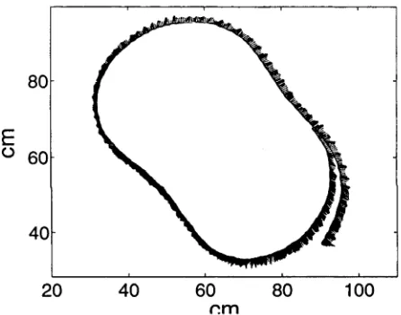
5-2 Actual arc contour and normal e s tim a te ... 76

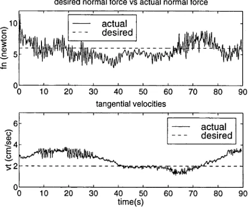
5-3 Normal forces and tangential velocities ... 77

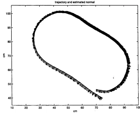
5-4 Actual contour shape and normal estim ate... 78

5-5 Normal forces and tangential velocities... 78

5-6 Parameter estimation with A = 0.97 79 5-7 Estimate of a with A = 0 .9 7 ... 79

5-8 Normal forces and velocities with A = 0 .9 7 ... 79

5-9 Forces and velocities without a d a p ta tio n ... 80

(13)

A-l Tool movement direction... 91

A-2 Determination of the control v elo cities... 91

A-3 Computation of new tool position using control v e lo c itie s ... 92

(14)

N o ta tio n

d d e p t h v a r i a b l e

D d e p t h c o n s t a n t

e f i e g} k u n i t v e c t o r s

f i n t e r a c t i o n f o r c e

f n n o r m a l f o r c e

In n o r m a l f o r c e c o n s t a n t

f t i f r t a n g e n t i a l f o r c e

f x t f y C a r t e s i a n f o r c e c o m p o n e n t s

k n o r m a l s t i f f n e s s

k j , k p g a i n c o n s t a n t

n n o r m a l v e c t o r

P p o s i t i o n v e c t o r

vc,v

t a n g e n t i a l v e l o c i t y c o n s t a n t s

v f v e l o c i t y a l o n g f

v <i v e l o c i t y n o r m a l t o f

V-xi Vy C a r t e s i a n v e l o c i t i e s

a i n c l u d e d a n g l e b e t w e e n f a n d r

A t t i m e i n c r e m e n t

A x x d i r e c t i o n p o s i t i o n i n c r e m e n t

A y y d i r e c t i o n p o s i t i o n i n c r e m e n t

A f o r g e t t i n g f a c t o r

ß , 7 , 5, C, C a n g l e v a r i a b l e s

t a n g e n t i a l k i n e m a t i c c o e f f i c i e n t o f f r i c t i o n

r , t t a n g e n t i a l v e c t o r s

(15)

6>1, #2 joint angles

(16)

A b b r e v ia tio n s

c c w

c o u n t e r c l o c k w i s e

C F A c o n t o u r f o l l o w i n g a l g o r i t h m

C F F c o n s t a n t f o r g e t t i n g f a c t o r

D A C d i r e c t a d a p t i v e c o n t r o l

D O F d e g r e e o f f r e e d o m

1 A C i n d i r e c t a d a p t i v e c o n t r o l

R L S r e c u r s i v e l e a s t s q u a r e s

S F A s u r f a c e f o l l o w i n g a l g o r i t h m

(17)

C h a p te r 1

I n t r o d u c t i o n

1.1 B a c k g r o u n d

A utonom ous cleaning in A ustralian heavy industry, p articu larly in the steel-m aking industry, is im p o rta n t. One exam ple is th a t a t present, B H P Steel spends ab o u t 8 m illion dollars per annum cleaning spilled m aterials in th e m aterials area of the P o rt K em bla Steel works alone. T he cleaning work is co n cen trated on th e removal of th e g ran ular m aterial from under and aro u nd p lant equipm ent such as conveyor belts. It is generally done by h and , using shovels and scrapers, exposing workers to heavy m anual lab o u r in d u sty and unhealth y conditions. So developing a u to m a te d cleaning system s can p o ten tially not only decrease costs for heavy in d u stry in A u stralia and over th e world, b u t also free th e workers from hostile and u n h ealthy environm ents. T his research is m o tiv ated by th e developm ent of such autonom ous cleaning system s.

T he environm ent is hostile to m any sensing facilities due to atm ospheric d u st, vari able lighting, acoustic and electrom agnetic noises. We believe th a t force sensing will play an im p o rta n t role because it has the advantages of being well-developed, reliable, econom ical, rugged and insensitive to noise above.

To remove th e g ranular m aterial by use of force sensing, th re e m ain problem s m ust be coped w ith: perceiving the granular m aterial, i.e., distinguishing it from o th er ob jec ts, such as a pillar, building walls and equipm ent shells; u n d e rsta n d in g th e in te rac tio n p ro p erties betw een th e tool and granular m aterials; and m oving th e ro b o t tool on th e surface while perform ing th e cleaning tasks. A vacuum cleaner will be a tta c h e d to th is spherical tool. T he tool moves(slides) on th e surface of a pile of gran u lar m

(18)

1.2. O R G A N I S A T I O N OF T H IS T H E S IS 2

als an d th e vacuum cleaner cleans th e m aterials sim ultaneously. T he first problem is beyond this research. O ur work concentrates on th e last two problem s.

1.2 O r g a n isa tio n o f th is T h e sis

(19)

C h a p te r 2

A M o d e l fo r I n te r a c tio n w ith

G r a n u la r M a te r ia l

2.1 In tr o d u c tio n

We are in terested in m an ip u latin g a robot tool to follow th e contours of an unknow n pile of g ranular m aterials. T he purpose is to clean granular m aterials effectively when an auto no m ous robotic cleaning system perform s a cleaning task in heavy industry. To in vestigate th is problem we have chosen to research th e force-m otion in teractio n betw een a spherical tool and a pile of granular m aterials(for our case, it is gravel). G ran u lar m aterials are ubiquitous in our daily life. A pile of gravel is only one exam ple. T hey consist of conglom eration of visible particles of different dim ensions. However, since each configuration of gran ular m aterials has its own characteristics, th e rep ro d u cib il ity of gran ular behaviour is poor [20]. T he problem how to m odel granu lar m aterials fru stra te s m any physicists and engineers [23]. We are not concerned w ith th e problem of how to purely m odel th e granular m aterial. W h a t we try to do is to o b tain some p ro p erties of a given pile of gravel when a ro bo t end-effector in teracts w ith it. We will app rox im ate a m odel to characterise th e in teractio n so th a t th e contour following control can be im plem ented effectively. Section 2 gives a concise description of the experim en tal system . An em pirical m odel s tru c tu re is proposed in section 3. Section 4 gives p a ra m e te r estim ation results. M odel verification is presented in section 5. Finally, conclusions are draw n.

(20)

2.2. EX PE R IM E N T A L SYSTEM 4

Figure 2-1: Experimental system setup

2 .2

E x p e r im e n ta l S y s te m

As shown in Figure 2-1, the experim ental system com prises an in d u strial CF-310 SCARA ro b o t, equipped w ith a 200 m m d iam eter spherical end-effector. We choose th is special tool because we expect th a t its size and geom etry will sim plify th e problem . T h e ro b o t is a typical in du strial robot w ith four degrees of freedom (D O F). We only use two jo in ts (links), base and elbow, for our experim ent. B oth base and elbow are equipped w ith an encoder and a tachom etre. T he robot is driven by a contro ller(a posi tio n controller or a velocity controller) running on V M E hardw are und er th e VxW orks o p eratin g system .

For force sensing, a JR 3 six-axis force to rq ue sensor is used to ob tain force d a ta . T he sensor is m ounted betw een th e tool and th e w rist. T his sensor m easures x, y and z forces an d m om ents (in force sensor fram e), althoug h we only use x and y force com ponents. T h e frequency of sam pling b o th force and position is 300 Hz.

[image:20.529.10.520.23.710.2]

(21)

2.3. M O D E L S T R U C T U R E FR O M Q U A L IT A T IV E E X P E R IM E N T S 5

two se n se d force com ponents fx and fy

position displacement(cm)

Figure 2-2: Two sensed force components / x(solid) and (dotted). Positive horizontal

coordinates correspond to contact depth.

2.3 M o d e l S t r u c t u r e f r o m Q u a l i t a t i v e E x p e r i m e n t s

As we m entioned previously, because of th e rich dynam ics of gran ular m aterials, it is alm ost im possible to precisely m odel all kinds of g ranular m aterials, or even a p a rtic u la r pile. O ur objective is to propose a feasible approxim ate m odel. A sim ple m odel can sim plify controller design and a complex m odel will m ake th e controller difficult to im plem ent. So it is preferable to get a suitable sim ple m odel to describe th e interaction s betw een granular m aterials and th e robot tool. We expect to use a low-order m odel. For exam ple, if a first-order m odel is used, th en stiffness an d dam ping p ro p erties of th e gravel should be determ ined. W ith this in m ind we conducted some initial experim ents to identify a sim ple b u t a p p ro p riate m odel.

(22)

2.3. MODEL ST R U C T U R E FROM Q UALITATIVE E X P E R IM E N T S 6

GRAVEL

Figure 2-3: Sensed force(fx. fy ). normal and tangential forces(ft . fn ), reference coordinates(X. Y).

is qu ite small. T his implies th a t when robot tool pushes a pile of gravel, th e norm al direction in teraction could be considered as a spring w ith a c o n stan t stiffness.

T h e tan g en tial force is tre a te d as arising from Couloum b friction which is th e p ro d u ct of norm al force and friction factor when a m ass moves on a plane. We also moved th e tool along a sloping plane of the gravel w ith ab o u t th e sam e d ep th . T he sensed ta n gential force was found to be relatively constan t for a constan t d ep th . O f course, if the d e p th is very sm all, th e sensed forces will be quite noisy. For sim plicity, th e tan g en tial force is taken to be p roportional to position displacem ent in th e norm al direction. So an em pirical m odel s tru c tu re is proposed as follows

fn = k d (2.1)

ft = /i d sign(t) (2.2)

(23)

2.4. MODEL PA R A M ET E R S ID E N T IFIC A T IO N 7

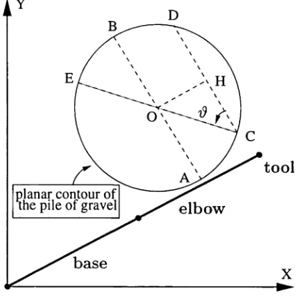
planar contour o f

the pile o f gravel _{e lb o w}

Figure 2-4: Determination of d

2 .4

M o d e l P a r a m e te r s I d e n tific a tio n

E x p erim en ts were th en conducted to identify values for th e two con stan ts k an d fi using least squares techniques.

In order to m ake th e two constants [i and k represent th e general pro p erties of the pile of gravel, we let th e tool push th e pile from different directions w ith different values

of d. Seven groups of d a ta are obtained. Each d a ta set was visually inspected to identify

th e in sta n t of co ntact and tru n c a te d to isolate th e d a ta associated w ith shallow -depth

interactio n s. T he actu al d ep th d was estim ated based on the displacem ent from th e

tim e of first con tact and knowledge of the actu al value of $. To m ake th e experim ental resu lts as reliable as possible, the shape of th e pile of gravel was m ade to be alm ost a cone, especially w ith a precise circular base. T h e two jo in ts(b ase an d elbow) are always aligned such th a t th e m ovem ent of the tool can be consider to be linear when th e d istance is only ab o u t a few centim etres as shown in figure 2-4. For shallow- d e p th co n tact, we can assum e th a t th e tool will move along line CD after it touches

po int C because th a t is the direction of the tool velocity before co n tact. So can be

approxim ately determ ined by th e following equation.

[image:23.529.165.381.104.321.2]

(24)

2.4. M O D E L P A R A M E T E R S ID E N T IF IC A T IO N 8

N ote th a t th e lengths of line O C (radius) and OH can be ap proxim ately got in advance.

T he least squares m eth od was th en applied to estim ate values using th e following form ulation.

From Figure 2-3 and applying force equilibrium , we have

f t = f x cos d - f y sin d

f n = f x sin d + f y cos d

We also can use f t and f n to express f x and f y

(2.4)

f x = f t COS d + f n sin d

f y = - f t s i n d + f n cos d

Using equation(2.1) and (2.2), equation (2.5) can be w ritte n in m atrix n o tatio n as (2.5)

where

*< II 6 (2.6)

X

45 II

f v ) T (2.7)

Ö =

{p

k)T (2.8)

I d cos d d s i n d \

(2.9)

\ — d sin d d cos d 1

an d d is th e con tact d e p th in th e norm al direction.

For a given •#, if we get m sam pling d a ta , th en equation (2.6) can be extend ed as

Fx y —

4? e

(2.10)

where

F*y = (f*yT(l) fxyT(2) f*yT(m ))T (2.11)

(25)

2.4. MODEL PA R A M E T E R S ID E N T IFIC A T IO N 9

Normal force(-) and its estimattion(-f). tangent force(o) and Its estimationf)

tangential

position displacement of end-effector (cm)

Figure 2-5: Comparison between (ft.. f n) and (f t * f n)

To get a general m odel, we use n different $ values for our experim ent and we have n equations in th e form of equation(2.10). G rouping th e n equations yields

Y xy = $ T 6> (2.13)

where

Y xy = ( F xyT ( l) F xyT (2) F xyT (n ))T (2.14)

<f = WT ( l) <f>T (2) (2.15)

A pplying least square estim ate algorithm produces

6 = (<Pr $ ) ~ 1 <Pr Y xy (2.16)

w here 6 is th e estim ate of 6. Using th e obtained d a ta to solve th e above equations, we o b tain the estim ates of fi and k

k = 16.25 N / c m

ji = 5.24 N / c m

N otice th a t k is m uch lower th a n th e tool stiffness(estim ated as a b o u t 100 N /c m ). T h is m eans th a t k is th e p ro p erty of th e gravel pile, instead of th e ro bot. Fig. 2-5 shows one exam ple of com parisons betw een actu al and estim ated norm al forces, and betw een actu al and e stim ated tan gen tial forces by use of k and (l for one experim ent w hen d is

(26)

2.5. MODEL V ERIFIC A TIO N 10

2 .5

M o d e l V er ifica tio n

A fter th e m odel p aram eter estim ates are known, we would like to use th e m odel to estim a te the d ep th d and th e angle d. Using equations (2.1) and (2.2), equatio n (2.4) can be rew ritte n as

cos d d f x f y fi sign(t)

sin d f x + f y

1 1 > 1

___

k

A pplying the trig identity sirred) + cos2(d) = 1 produces

(2.17)

d

n+f

,?

/ i2 - f k2 (2.18)

If p a ram eters k and [i are known, th en equations (2.17) and (2.18) can be used to

estim a te d and d on line. Note th a t equation (2.17) becomes ind eterm in ate when the

sensed forces are too small. B ut this case can be elim inated by a thresh o ld criteria. Also notice th a t the solution of the equation (2.17) is depen dent on sig n (t) which has two possible values. T his am biguity can be solved by assum ing th a t sig n (t) is eith er 1 or -1,

th e n checking the tan gen tial velocity calculated by th e resulting d. If it is consistent

w ith th e assum ption, th en th e assum ption is correct. O therw ise, th e alte rn a tiv e of sig n (t) should be used.

By choosing different d values which are determ ined by th e m etho ds in th e previous

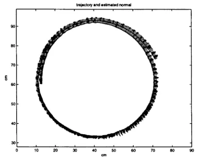
section as shown in figure 2-4, we got seven groups of d a ta . Figures 2-Ö-2-7 show th e b est an d th e worst of th e results. Obviously, th e results illu strate th a t th e estim ated d e p th an d th e estim ated angle d( which tells us th e surface norm al) are q u ite near th e tru e values. T his m eans th a t th e m odel is ap p ro p riate and acceptable.

2 .6

C o n c lu sio n

(27)

2.6. C O N C L U S I O N 11

actual depth vs. estimated depth

5 0.2 0.25 0.3 0.

time(s)

actual vartheta vs. estimated vartheta

0.25 time(s)

F ig u re 2-G: Best, e s tim a tio n re su lts

actual depth vs. estimated depth

estimated depth actual depth

5 0.2 0.25 0.3 0.

time(s)

actual vartheta vs. estimated vartheta

time(s)

(28)

C h a p t e r 3

C o n to u r F o llo w in g C o n tr o l

3.1 I n tr o d u c tio n

In this ch ap ter, we focus on realizing th e ro bo t tool m ovem ent over th e surface of th e pile of gravel. T his is novel research work, since to th e a u th o r”s knowledge no sim ilar work has been carried out previously. It is also im p o rta n t. W hen th e robot system whose tool is equipped w ith a vacuum cleaner perform s a cleaning task , th e tool should move on th e surface of th e pile of granular m aterials ra th e r th a n go inside th e pile. Based on the proposed contour following control algorithm , we have done a lot of sim ulations and experim ents. T he results d em o n strate th a t th e rob ot tool can move over th e different planar contours of th e pile of gravel satisfactorily.

In th is ch ap ter, we first give a review on robotic surface following control. T h en we p resent a sim ple contour following algorithm . Some sim ulation results are th e n given. F inally experim ental results are presented to show th e effectiveness of th e contour following algorithm (C FA ).

3 .2

L ite r a tu r e R e v ie w

T here are m any applications which require th e robot m an ip u lato r to in te rac t w ith th e environm ent, especially to follow the shape of the environm ent during perform ing its task. T hese applications include surface polishing, grinding, scraping, m achining, sheep shearing, and so on. Accordingly, th ere are some surface following algorithm s(SFA ) in th e litera tu re . Based on th e different environm ental characteristics, two m ain SFA

(29)

3.2. LITERATURE R EVIEW 13

strateg ies exist. One is for dealing w ith rigid surfaces and th e oth er is to tackle th e soft surfaces. Here soft m eans th a t th e environm ent is deform able.

In some previous works on robot force/positio n control, th e surface m odel of th e object was given or obtained by various m ethods to allow estim atio n in advance[16][17]. Recognising th a t it is very tim e consum ing in com puting to get a global m odel, R .E. G o d d ard et al[14] proposed a control m ethod for ro b o t rolling and sliding over an u n known o bject. T his m eth od makes use of velocity control ra th e r th a n position control. Using velocity control for ro b o t probing only needs local inform ation instead of a global m odel of th e object. In ad d itio n , holonomic and non-holonom ic con strain ts were con sidered for m otion planning of robot fingers. B ut only sim ulations were done to show th e effectiveness of th e control algorithm .

In order to move a robot end-effector over th e surface of an o b ject, some inform a tion a b o u t the surface locally or globally m ust be o btained. Some researchers have m ade efforts to estim ate th e co n strain t surface for force control. Merlet[27] proposed a m eth o d which used force m easurem ents to determ in e th e force norm al. B lauer and Belanger[3] proposed using an extended K alm an filter to estim ate some unknow n p a ram e te rs related to th e co n strain t surface. Kazanzides[22] m ade use of in teractio n force an d end-effector velocity to d eterm ine the co n strain t surface norm al and tan g en tial di rections. In the m eth o d proposed by T. Yoshikawa and A. Sudou[54], b o th force and position m easurem ents were utilized to estim ate th e co n strain t surface locally on-line. T h is m eth o d dealt w ith th e three-dim ensional space directly. In ad d itio n , a stra te g y was taken to com pensate th e frictional force. Finally, experim ental resu lts using a SCARA robot were presented to show the good com bination betw een th e online esti m atio n algorithm and the dynam ic hybrid control.

If th e force controller is equipped w ith a low-friction roller, th en th e m easured force a t th e surface is m ostly th e norm al force. Also th e norm al force and th e tan g en tial

force have a sim ple relation. D. B ossert et al[5] presented a SFA which m ade use of

(30)

3.3. CONTOUR FOLLOWING ALGORITHM

14

6 is a free p aram eter

Figure 3-1: Object, contour

using th e PU M A in d u strial robot to verify th e preview control. Some o th er surface following algorithm s were proposed in [31] [32] [33].

However, all of th e above m entioned references are based on th e fact th a t th e object surface is rigid. How to move th e robot end-effector over th e surface of a pile of granu lar m atericils(or griwel for our situ atio n ) is a new topic. D ifferent from th e rigid surfaces, th e surface of a pile of granular m aterials has its own unique characteristics. One obvious aspect is th a t th e surface is rough, a n o th e r pro p erty is th a t when th e end- effector pushes th e pile, th e local shape will be deform ed perm anently. So when th e ro bo t end-effector moves on th e surface of a pile of granular m aterials, some m aterials will be pushed aside and th e surface shape will be changed.

3.3 C o n t o u r F o llo w in g A lg o r ith m

In th is section, we will derive a surface following control algorithm . T his algorithm m akes use of control velocity to ad ju st th e moving trajecto ry .

Figure 3-1 shows th e plan ar contour of a pile of granular m aterials. Let th e p a ra

m etric curve r($) represent the b ou n d ary of th e pile of gravel. Assum e |r(0)| ^ 0.

(31)

3 .3 . C O N T O U R F O L L O W I N G A L G O R I T H M 15

(3.1)

n(0) = k x r(<9) (3.2)

w here k is th e u n it vector th a t points out of the paper.

Using th e m odel deduced in th e previous ch ap ter, the in teraction force exerted on th e environm ent by th e tool can be rew ritte n as

w here d, k and fi have th e same definitions as before w ith d, th e actu al d e p th in

norm al direction; fc, norm al direction stiffness coefficient; /i, tan g en tial direction force coefficient.

T h e control objective is to move th e end-effector over th e plan ar contour of gravel w ith th e desired norm al force an d tangential velocity. T his aim can be expressed as

w here is th e desired norm al force, p is th e position vector of th e ro b o t tool, and Vc is th e desired velocity.

N aturally, we can change th e tool velocity in th e surface norm al to a d ju st th e norm al force. So we use th e following control law.

elsewhere d > 0

(3.3)

f • n(0) = /n n{6)

IpI = Vc

(3.4)

p = Vc t + kf (Jn - /» ) n (3.5)

w here k f is a gain co n stan t, / „ is th e m easured norm al force. E q u atio n (3.5) can also be w ritte n as

(32)

3 .3 . C O N T O U R F O L L O W I N G A L G O R I T H M 16

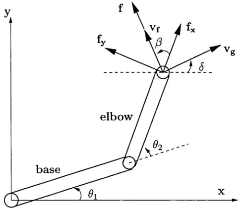
Figure 3-2: Determination of the control velocities

w here kp is a gain co n stan t which is equal to kf k, D is d e p th co n stan t which equals

f N/ k.

Let e be force tracking error, we have

e = f nn - f Nn

T he above control law satisfies

(3.7)

Proof:

(e + kf ke) • n = 0 (3.8)

(e + kf ke) • n / « n + k kf ( f n - f N)

k d n + k k f ( f n - f N)

k{p - r(0))n + k kf ( f n - f u)

k p n + k k f ( f n - f N)

kVct n + k k f ( f N - f n) + k k f ( f n - /n)

0

T h e control law(3.5) is a little awkw ard to im plem ent because th e c o m p u ta tio n

related to th e coordinate (t, n) will be relatively com plex. Now we give a m ore conve

(33)

3.3. C O N T O U R F O L L O W I N G A L G O R I T H M 17

sensed force, th e norm al and th e tang en tial, e f and e q are u n it vectors, ey is along the

force direction and is norm al to ey. O ur purpose is to factorise th e velocity p into

two velocity com ponents, l.e.Vf and vq . They are in th e sam e directions as u n it vectors

ey and e,7 respectively. T he velocity com ponents (Vf, vq) are referenced to co ordinate

system (ey, e,7) which is easy to determ ine by:

I e,

= f / |f |

1 e <7 = - k x e /

w here k has th e same definition as in equation(3.2).

From figure 3-2, we get

P = ( p - e / ) e / + ( p - e , 7)e,7

= (Vct + k f ( f N - /„ ) n) • ey e / + (Vct + k f ( f N - /„ ) n) • e q e q

= {Vct • ey + k f ( f N - f n) n • e f ) e f + (Vc t ■ e fl + k f ( f N - / „ ) n • e g) e q

= (Vc cos a + k f { /n ~ f n) s in a) e / + {Vc sin a - k f ( f N - /„ ) cos a) e q

Assum e th a t Vf and v qare two velocity com ponents along ey and e (/, respectively. T hen

we have

Vc

k f { /n ~ f n )

S u b stitu tin g f n = | / | s in a into the above equation yields cos a s in a

s in a —cos a

(3.9)

cos a sin a \ ( Vc

s i n a —c o s a I V k f ( f w — \ f \ s i n a )

Obviously, Vf and vq are functions of |f| only which can be m easured online. So

th is control law is m uch easier to im plem ent th a n control lay(3.5). N ote th a t only a which equals t a n ~ 1{k/ ^ ) , not k or /i, actually ap p ears in th e above control law.

(34)

3.3. C O N T O U R FOLLOWING ALGORITHM 18

Figure 3-3: Determination of the force and velocity tracking errors

U nder these conditions, th is robot system will quickly reach th e steady s ta te after th e CFA is executed. W hen the system is in the steady s ta te , th e tan g en tial velocity is co n sta n t and th e norm al velocity of the tool is zero. So we have

cos a s m a

sin a —cos a

w here Vt is th e actual tan gen tial velocity.

In ad d itio n , as th e estim ated a is used, the control law becomes

(3.10)

cos a s in a

s in a —cos a

where f n is th e estim ated norm al force.

Com bining equation(3.10) an d (3.11) yields

cos a V t + k f s in a f n = cos a V c + k f fn s in a

sin a V t — k f cos a / „ = s in a V c — k f fn cosa

Solving th e above equation produces

Vt = — ^ —

f n = In - $ t a n { ( i - a )

(3.11)

(3.12)

(35)

3.4. CONTROL SYSTEM ST R U C T U R E 19

R O B O T

FO R C E SE N SO R V E L O C IT Y

C O N T R O L L E R N Y T R O N M E N T

Figure 3-4: Block scheme of velocity control

Vt =₁ ----^ ----_{cos( ä}_{— « )}

I n — { In — j fj t an(a — a ) } s i n a / sin a

(3.13)

w here f n is the actu al norm al force m agnitude.

So we can approxim ately predict th e force an d velocity tracking errors provided th a t we know th e error of th e estim ated a .

3. 4

C o n t r o l S y s t e m S t r u c t u r e

In th e previous section, we derived a contour following algorithm using force feedback for velocity com pensation. In this section we explain how th is algorithm can be applied to a real robot.

T he m ost n a tu ra l way is to use th e algorithm to drive a ro bo t u n d er close-loop velocity control as shown in figure 3-4. A nother way is to use it to drive a ro b o t u n d er velocity-based position control as shown in figure 3-5 and figure 3-6. In a d d itio n , we can im agine m ore soph isticated approaches to control. For exam ple, th e m an ip u la to r dynam ic m odel can be used for th e control objective, b u t we choose n ot to consider th e m unless necessary.

C om paratively th e system shown in figure 3-4 is sim pler. T he close-loop velocity control can be im plem ented directly. B ut the velocity controller of our robotic system has not been satisfactorily im plem ented.

(36)

3.4. CONTROL SY STEM ST R U C T U R E 20

R O B O T

FO R C E S E N SO R

C O N T R O L L E R P O S IT IO N K IN E M A T IC S

IN V E R S E

E N V IR O N M E N T

Figure 3-5: Block scheme one of velocity-based position control

K I N E M A T I C S F O R W A R D

F O R C E S E N S O R K I N E M A T I C S

I N V E R S E

C O N T R O L L E R E N V I R O N M E N T

Figure 3-6: Block scheme two of velocity-based position control

th e tracking will fail due to lose of co ntact, or too great a d e p th . O ur approach to solve th is problem is to use th e present position inform ation as well as th e control velocities for th e co m p u tatio n of th e next position of the end-effector. T he idea is illu strate d in figure 3-6.

Notice th a t the proposed controllers are driven solely by force m easurem ents. T he surface norm al and tan g en tial are com puted by force m easurem ents as well as position inform ation. Also notice th a t th e controllers do not include a dynam ic m odel of th e m an ip u lato r. We have chosen to im plem ent th e contour following control w ith a sim ple velocity-based position control. It is expected th a t th e perform ance would be im proved w ith a m odel-based ro b o t m otion controller(e.g. com pu ted-torqu e). B u t we have found th a t it is not necessary to use a sophisticated controller to get good results.

Now let us use figure 3-7 to determ ine th e next position th e end-effector should move to from th e p resent point.

From figure3-7, we have

5 = ß + 01 + 02 - p i / 2 (3.14)

(37)

3.5. DIGITAL FILTERING 21

e lb o w

Figure 3-7: Computation of new position using control velocities

T h e n we have th e relationship betw een the v e lo c itie s ^ /, vfl) and (vx , vy).

vx = cos 8 vq — s in 8 Vf

vy = sin 5 vg + cos 8 Vf

w here vx and vy are two next desired C artesian velocities.

F u rth erm o re, th e C artesian position increm ents are

A X = vx A t I A y = vy A t

w here A t is the tim e increm ent. Finally, we o b tain th e next position

n e w — •Eold " t ” A X

Vnew — Void "F A y

(3.15)

(3.16)

(3.17)

A pplying th e inverse kinem atics, we can tran sfo rm th e C artesian position into jo in t posit-o n to carry out th e jo in t space position control.

3.5 D igital Filtering

[image:37.529.153.398.99.310.2]

(38)

highest and lowest cutoff frequencies of 500H z and 0 A 8 8 3 H z respectively. We choose

th e b u ilt-in filter w ith cutoff frequency of 31.2H z . T his selection is based on th e fact th a t th e actual sam pling frequency of b o th position and force in our experim ents is a b o u t 10 to 20 Hz. Also it is desirable to a tte n u a te the noises as m uch as possible. However, we find th a t th ere still exist rich noises in th e filtered force m easurem ents w ith any b u ilt-in filter. So it is desirable to design a digital filter to sm ooth th e tra je c to ry of th e end-effector and furth erm o re to suppress some high frequency noises on-line.

F ilterin g is used to e x tra ct signals from noise. If the signal and noise sp e ctra are not overlapping, it is possible to design a filter to pass th e desired signals and to remove th e unw anted noises. If the signal and noise fields are p a rtly overlapping, it is expedient to suppress th e noises w itho u t a tte n u a tin g the signals largely.

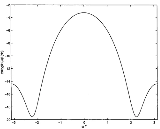
T here are three basic classes of digital filters. T hey are fast tran sfo rm filters, n o n recursive filters and recursive filter. Fast transfo rm filters im plem ent th e generalised frequency response of th e digital filter using fast tran sfo rm algorithm . T h e F F T fil ters are the best known of such filters. Recursive and nonrecursive filters realize th e

frequency response H{ z ) in hardw are using delays, scalers and sum m ers, or in m i

croprocessor hardw are. These filters can also be im plem ented in software by use of sets of recursion equations. Recursive filters are often referred to as infinite im pulse response(IIR ) filters. H R filters norm ally require less hardw are and can carry o ut fil tering tasks m ore quickly th a n finite im pulse response(F IR ) filters often referred to as nonrecursive filters. However, nonrecursive filters are inherently stable. T hey can also be designed to have a linear phase pro p erty in th e passband.

For sim plicity, we design a F IR filter using windowing and tru n c a tio n technique [4]. T his filter is used to remove some high frequency noises from th e force m easurem ents. It can also sm ooth th e tra je c to ry of th e end-effector. Now let us consider a filter whose in p u t-o u tp u t behaviour is described w ith the following difference equation.

y { k) = a x { k ) -f b x ( k — 1) + c x ( k — 2) (3.18)

Here designing a filter m eans to determ ine th e coefficients a, b and c. Consider th e

frequency response function H ( e JU}T) for an ideal lowpass filter whose cutoff frequency

(39)

[image:39.529.147.404.131.401.2]

Figure 3-8: Lowpass filter characteristics

[image:39.529.151.407.490.698.2]

(40)

3.5. DIGITAL FILTERING

24

<oT

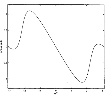
Figure 3-10: Phase of the frequency response of the designed filter

25

20

15

10

5

0

0 20 40 60 80 100 120 desired normal force vs actual normal force

--- actual desired

tlme(s) the actual tangential velocity

[image:40.529.162.391.147.352.2]

(41)

3.5. DIGITAL FILTERING

25

desired normal force vs actual normal force

— _c10

0

lime(s) the actual tangential velocity

100 120

time(s)

Figure 3-12: Experimental results (circular contour)without using the designed filter

Using Fourier series expansion for H( e JujT) yields

OO

H{eJojT) = h{ k ) e ~ihjjT

fc= —oo

Then the impulse response function can be calculated by

h ( k) = <

s i n [ ( k —kp) ujc T\

( k - k 0) 7T k 7^ ky

k = k()

(3.19)

where ko is a constant. For brevity, we take ko=0. If u>c — 9H z and T = 0.1 s, then a = h(0) = 0.286, b = h( 1) = 0.25 and c = h (2) = 0.155. The actual m agnitude and phase of the frequency response of the designed filter are shown in figure 3-9, 3-10. The frequency roll-of of this filter is about 108 db/decade.

(42)

3.6. SIM ULATIO N RESULTS 26

Figure 3-13: Simulation using elliptical contour

3.6 S im u la tio n R e s u lts

In th is section, we first give some sim ulation results by use of an ideal v irtu al rob ot. T h en th e sim ulation results using a real robot are presented. T here exists a difference betw een these two sim ulations. T he ideal v irtu al ro b o t can perform a positioning task w ith o u t any error. B u t th e actual ro b o t norm ally cannot reach th e desired position exactly, p articu larly when th e tim e interval is very small. So it is necessary to present b o th sim ulation results. T he second case is actually a hybrid com bination of sim ulation and experim ent. T he robot is real and m otion d a ta is experim ental.

3.6 .1 S im u la tio n U sin g V ir tu a l Id eal R o b o t

In th is subsection, we assum e th a t th e robot can perform tracking task w ith o u t any positioning error. In order to deal w ith the general situ a tio n , we use an ellipse as th e p lan ar contour of a pile of gravel as shown in figure 3-13.

Assum e th a t p c{xc, y c) is the ellipse canter, point p t is th e present position of the

tool, an d p\ and p2 are two points on th e contour. In order to com pute th e sensed

(43)

7 = atan2 (yt - yc, x r - xc) (3.20)

Then the coordinate at p\ can be calculated by

x\ = a cos 7 + x c

yi = b sin 7 + yc

(3.21)

where a and b are major and minor axes. According to the properties of ellipses,

the equation of the normal at p\ is

(x - x c) a? _ {y - yc) b2

~ x c yi - yc

Equation(3.22) can be rewritten as

(3.22)

where

y = A x + B

A = a?/b2 tan(y)

B = yc ~ (xc + x i (a2/b2 - 1)) tan(7 )

So the equation of the normal at p2 is

(3.23)

y = A x + C

where C = y i — A X j . The equation of the ellipse is

(x - xc)2 (y - yc)2 _

a? b2

Substituting equation (3.24) into equation (3.25) yields

M x2 + N x + L = 0

(3.24)

(3.25)

(44)

trajectory of robot end-effector

cm

Figure 3-14: Simulation using exact model parameters

where

M = b2 + ( a A ) 2

N = - 2(b2 x c + a 2 A y c - C ))

L = ( b x c)2 + a2(yc - C ) 2 - ( ab) 2

Solving equation (3.26) for X2 and th e n solving equatio n (3.24), we obUtin th e

coordin ate P2(x 2,y2)- Now th e d e p th can be calculated w ith

d = y / ( x 2 ~ X i) 2 + (V2 ~ V i ) 2 )

Notice th a t th ere are two solutions for xo and yo- Accordingly, d has two values.

T he larger value should be discarded. Using f n = k d to com pute f n and th e n using

equation (3.9) to calculate Vf and vq, finally, we can determ ine th e new position by

x n e w — x old ~ v f cos ^ A t — Vq S i nA A t ynew = Void - V f s in \ A t + vq cos A A t

(3.27)

where A = a t a n ( A) + a — 7r/2, a is a known co n stan t which is th e angle betw een the co ntact force and th e surface tang ential.

(45)

Actual normal force vs the desired normal force

time(s)

Actual tangential velocity vs the desired tangential velocity

30

time(s)

Figure 3-15: Simulation using exact model parameters

we add random noise to th e force signals. T his noise is rand om num bers which are

p roduced by th e sta n d a rd C rand function. T he m agnitu de of these random num bers

is betw een 0.2 New ton and -0.2 N ew ton. T he random noise is also used in the following subsection.

W hen th e actual and estim ated p aram eters are assum ed to be th e sam e w ith fc(normci\ stiffness coefficient)= 12.0 N /c m and ^ (ta n g e n tia l force coefficient) = 10.55 N /c m , th e sim ulation results are shown in Figures 3-14-3-15. T he corresponding tru e

a is 48.68 degree. Figures 3-16-3-17 show th e sim ulation resu lts when th e estim ated

m odel p a ram eters are different from the real ones w ith K e=15.2 N /c m and [ie=8.2

(46)

actual normal force desired normal force

0 20 30 40 50

time(s)

Figure 3-1G: Simulation using estimated model parameters(without noises)

I

z

time(s)

(47)

3.6. SIMULATION RESULTS

31

3 .6 .2 H y b rid S im u la tio n U sin g R ea l R o b o t

T he sim ulation in th e above subsection can be tre a te d as perform ed by use of an ideal ro bo t to execute p o int-to -po in t m ovem ent w ith o u t any error. Now we use th e SC A RA ro bot to realize th e desired po in t-to-p oint m ovem ent. Here th e real ro bot is in teractin g w ith a sim ulation of th e pile of gravel. All of th e m odel p a ram eters are th e sam e as in th e above subsection w ith k = 12.0 N / c m , y = 10.55 N / c m an d a = 0.85 rad.

Let th e sam pling period be T. T he sam pling frequency can be set up by frequency sp littin g . For exam ple, th e sam pling frequency 20Hz can be produced by dividing the servo r a te (300 Hz) by 15. T h en th e actual C artesian velocities are

where Ax(i) and Ay(i) are actu al C artesian position displacem ents a t th e zth sam

pling point. Notice th a t th e tim e increm ent A t and T are tre a te d th e sam e in the previous section when th e ideal virtu al robot is used. B u t for actu al situ a tio n , we can tre a t th em separately to get b e tte r control results. Here A t is used to com pute position

increm ent by use of th e known control velocity com ponents Vf and vg. If we use T to

calculate th e C artesian position increm ent w ith A x = vx T an d A y = vy T, th e incre m ent will be very small. T his will result in poor tracking perform ance, or even track ing failure w ith th e real robot. We found th a t th e tool velocity will decrease quickly until

near zero an d there will be a large error in force tracking too. Normally, A t should be

m uch larger th a n T. T he following results will d em o n strate th a t th e ap p ro p riate A t is ab o u t 0.9 s and T is a b o u t 0.1 to 0.05 s.

Using th e estim ated tan g en tial direction, we can o b tain th e actual tan g e n tia l ve locities by use of th e C artesian velocities. Note th a t th e m entioned tan g en tial velocity here is different from th e desired velocity Vc. T h ro u g h o u t all of th e sim ulations and experim ents in th is thesis, Vc is equal to 2cm /sec. Vc is th e desired tan g en tial velocity when th e velocity closed-loop system is used. T he velocity feedback closed-loop sy stem tries to a d ju st th e o u tp u t velocity to the given value. Since th e position control is

used, th e velocity will be dep end ent on th e sam pling period T an d th e tim e increm ent

A t as well as gain co n stan t kf. Large tim e increm ents will bring a b o u t large velocity. T he late r sim ulation and experim ental results will d em o n strate th a t even th o u g h th e

(48)

time(s) the actual tangential velocity

time(s)

Figure 3-18: Simulation results with kf = OAcm/ s/ N. A t = 1.0s and T = 0.1s

time(s)

Figure 3-19: Simulation results with kf = 0 . 7cm/ s /N. A t = 1.0s and T = 0.1s

time(s)

(49)

time(s)

Figure 3-21: Simulation results with kf = 0.7Gcm/s/ N, At = O.O.s and T = 1/G.s

position control approach is used, th e resu lta n t tangential velocities will be near th e desired values if A t, T and k f are ap p ro p riately chosen.

Choosing control system p aram eters is im p o rta n t in th e system design. C ontrol

perform ance will be greatly affected by the controller p aram eters which are k f, A t and

T for our case.

Figures 3-18-3-20 illu strate th e sim ulation results when th ree different gain con sta n ts, i.e. 0.4, 0.7 and 1.0 c m /s /N are used. T he sam pling frequency and tim e incre

m ent are 10 Hz and 1.0 s respectively. Theoretically, large gain k f will increase control

sensitivity and ad ju stm e n t. B u t very large gain will also result in large oscillation and even un stab le. On the o ther h an d , th e ad ju stm e n t perform ance will be poor w ith sm all gain. T h e results shown in Figures 3-18-3-20 tally w ith th e theory. For th e given A t and T , th e suitable gain co n stan t k f is betw een 0.7 and 1.0.

T h en we determ in e w hat is th e suitable sam pling frequency. T h e resu lts w ith four

different frequencies are shown in Figures 3-21-3-23. T he gain k f an d tim e increm ent

A t are 0.76 c m /s /N and 0.9 s respectively. W hen k f and A t are th e given values, th e a p p ro p riate sam pling frequency is betw een 10 and 20 Hz. W hen sam pling frequency is over 150 Hz, th e contour following control will fail. On the oth er h an d , w hen th e frequency is lower th a n 6Hz, th ere exist large oscillations.

F u rtherm ore we use different tim e increm ent to u n d e rsta n d its effect upon th e sys tem perform ance. T he results are illu strated in Figures 3-25-3-28.

(50)

the actual tangential velocity

Figure 3-22: Simulation results with kf = 0.76cm/s/N. At = 0.9s and T = 0.1s

time(s)

Figure 3-23: Simulation results with kf = 0.76cm/s/N, A t = 0.9s and T = l/3 0 s

20 25 30

25

time(s)

(51)

time(s)

Figure 3-25: Simulation results with kf = 0. 7 c m / s/ N. A t = 0.7.s and T = l/15.s

20 25 30

time(s) ttie actual tangential velocity

time(s)

Figure 3-2G: Simulation results with kf = 0 . 7 c m / s / N . A t = l.O.s and T = l/1 5 s

15 20 25

timefs) the actual tangential velocity

time(s)

(52)

10

time(s)

Figure 3-28: Simulation results with kf = 0 . 7 c m / s / N . A t = 2.2s and T = 1/lS.s

actual tool locus

Figure 3-29: Simulation results with kf = 0.7cm/s/N, A t = l.O.s and T = l/1 5 s

It will easily resu lt in tracking failure in an actual situ atio n . It is wise to choose tim e increm ent aro u n d 1 s.

Figure 3-29 shows th e actu al tool locus when k f = 0.7 c m / s / N , A t = 1.0 s and

T = 1/15 s. Since th e d e p th is m uch sm aller com pared to th e elliptical m ajo r or m inor axis, th e tool tra je c to ry is still sm ooth. Because th e tool locus for o th er cases are alm ost th e sam e as th is one, it is n ot necessary to show them .