Rochester Institute of Technology
RIT Scholar Works
Theses
Thesis/Dissertation Collections
11-3-2009
Investigation of tetrahedron elements using
automatic meshing in finite element analysis
Gordon Bae-Ji Tseng
Follow this and additional works at:
http://scholarworks.rit.edu/theses
This Thesis is brought to you for free and open access by the Thesis/Dissertation Collections at RIT Scholar Works. It has been accepted for inclusion
in Theses by an authorized administrator of RIT Scholar Works. For more information, please contact
Recommended Citation
Investigation of Tetrahedron Elements
Using Automatic Meshing in
Finite Element Analysis
Gordon Bae-Ji Tseng
A Thesis Sllmmitted in partial fulfillment
of the
Requirments for the degree of
Master of Science
in
Mechanical Engineering
Rochester Institute of Technology
Rochester, New York
August 1992
Approved by:
Dr. Joseph S. Torok (Advisor)
Dr. Rober Hefner
Dr. Mark Kempski
Acknowledgment
I
dedicate
this
workto
my Mother
andFather,
whohave
providedsupport and encouragement
to
allowmeto
accomplishthis
achievement.I
wouldlike
to
thank
Dr. Joseph
Torok,
my
advisor,
for
guidance ,valuable suggestions and
for
alwaysbeing
availablefor
assistance.He is
a great professor andfriend.
I
wouldlike
to thank
allthe
members ofthe
RIT
Mechanical
Engineering
Department
whohave
been very helpful working
with methrough
the
schoolyears.
Thesis
Outline
Abstract
Table
ofContents
Chapter
1.
Introduction
Geometric
Modelers
1)
Wire
frame
modelers2)
Surface
modelers3)
Solid
modelersConstructive Solid
Geometry
(CSG)
Boundary
Representation
(bRep)
Cell
Decomposition's
andSpatial
Enumeration
Approaches
to
mesh generationLaplacian
methodMapping
methodsAutomatic
meshgeneration1. Point
placementfollowed
by
domain
triangulation
2.
Mesh
generationbased
on sub-domain removal3. Mesh
generationby
recursivesubdividing
4.
Spatial
decomposition followed
by
sub-domain meshControl
ofthe
elementdistribution
Chapter 2.
Test Problems
Static State
Modal
analysisChapter 3.
Analytical
Solutions
Cantilever
(square)
beam
Cantilever
(round)
beam
Square
flat
plate all edgesfixed
Circular
flat
plate with a edgefixed
Chapter 4.
FEA
Results
Cantilever
(square)
beam
Cantilever
(round)
beam
Square
flat
plate all edgesfixed
Circular flat
plate with a edgefixed
Chapter
5.
Discussion
ofResults
Cantilever
(square)
beam
Cantilever
(round)
beam
Square
flat
plate all edgesfixed
Circular
flat
plate with aedgefixed
Chapter
6.
Conclusion
Chapter 7.
Summary
Abstract
This investigation
examinesthe
quality
offinite
element analysis(FEA)
resultsbased
onthe
use oftetrahedron
elements.For
some classes of problems analyzedby
the
finite
element method(FEM),
the
use of various polynomial ordertetrahedra
is
consideredquite acceptable.However,
in
other classes ofproblems,
particularly
stressanalysis,
usershave
astrong
bias
againstthese types
of elements.Various
case studiesare
performed,
comparing
resultsbased
on severaltypes
ofthree-dimensional
elements.Page11
Table
ofContents
List
ofFigures
Pg-
iv
List
ofTables
Pg.
ix
Chapter 1.
Introduction
Pg-
1
Chapter 2.
Test
Problems
Pg-
21
Chapter 3.
Analytical Solutions
Pg.
23
Chapter 4.
FEA Results
Pg-
29
Chapter
5.
Discussion
ofResults
Pg-
314
Chapter 6.
Conclusion
Pg-
342
Chapter
7.
Summary
Pg-
371
List
ofFigures
Figure 1.1 Wire
frame
representationFigure 1.2 Constructive Solid
Geometry
modelerFigure 1.3
Boundary
representation modelerFigure 1.4
3-dimensional
octree modelerFigure 1.5 A
3-dimensional
mapping
mesh generationFigure 1.6 Dirichlet
tessellation
andDelaunay
triangulationFigure 1.7
Watson's
Algorithm
Figure 1.8 A way
to
define
the
node pointsin
spaceFigure 1.9 The
distorted
Delaunay
tetrahedron,
"silver"
Figure 1.10
Surrounding
algorithmFigure 1.11 The flow
chart ofthe
3-dimensional
surrounding
algorithm
Figure 1.12 The
"Ghost"pointfor
boundary
definition
Figure 1.13 Subdivision
of a multilateraldomain
Figure
1.14.
Nodal
levels
Figure 1.15
Element
removal operatorsFigure 1.16
Cutting
concave polygonusing splitting line
Figure 1.17 chopping
offlayers
yield elementsFigure
1.18
The
quadtree and modified quadtree representationsFigure
1.19
Examples
of cut octants usedin
the
modified octree algorithmFigure 1.20 A
overview of octree/Delaunay
triangulation
methodFigure
2.1 Cantilever
(square)
beam
Figure
2.2 Cantilever
(round)
beam
Figure
2.3 Square flat
plate all edgesfixed
Figure
2.4 Circular flat
plate with a edgefixed
Figure
3.1 Cantilever
(square)
beam
Figure
3.2 Cantilever
(round)
beam
Figure
3.3
Square
flat
plate all edgesfixed
Figure
3.4
Mode
1
Figure
3.5
Mode
2&3
Figure
3.6
Mode
4&5
Figure
3.7
Mode
6
Figure
3.8 Circular flat
plate with a edgefixed
Figure
3.9
Mode
1
Figure
3.10
Mode
2&3
Figure 3.11 Mode 4&5
Figure 3.12 Mode
6
Figure
4.1 Type
of elementsFigure
4.2
Maximum
displacements
w/
40
LQ
elements.Figure
4.3
Maximum
displacements
w/
320
LQ
elements.Figure
4.4
Maximum
displacements
w/
40
Figure
4.5
Maximum
displacements
w/
320
Page
iv
Figure 4.6 Maximum
displacements
w/
71 LT
elements.Figure 4.7 Maximum
displacements
w/
532 LT
elements.Figure 4.8 Maximum
displacements
w/
703 LT
elements.Figure 4.9 Maximum
displacements
w/
4095 LT
elements.Figure 4.10 Maximum
displacements
w/
7947
LT
elements.Figure 4.11 Maximum
displacements
w/
71 QT
elements.Figure 4.12 Maximum
displacements
w/
532
QT
elements.Figure 4.13 Maximum
displacements
w/
703 QT
elements.Figure 4.14 Maximum displacements
w/
65
LQ
elements.Figure 4.15 Maximum
displacements
w/
221
LQ
elements.Figure 4.16 Maximum displacements
w/
432
LQ
elements.Figure 4.17 Maximum displacements
w/
703
LQ
elements.Figure 4.18 Maximum displacements
w/
48
Figure 4.19
Maximum
displacements
w/
192
Figure 4.20 Maximum displacements
w/ 77
LT
elements.Figure 4.21
Maximum
displacements
w/
328
LT
elements.Figure
4.22 Maximum
displacements
w/
659
LT
elements.Figure 4.23
Maximum
displacements
w/
1937 LT
elements.Figure 4.24 Maximum
displacements
w/
5977 LT
elements.Figure 4.25 Maximum
displacements
w/
77
QT
elements.Figure
4.26
Maximum
displacements
w/
328 QT
elements.Figure 4.27-4.32
Square
flat
plate model and mode1-5
mode shapew/
25
LQ
elements.Figure
4.33-4.38 Square
flat
plate model and mode1-5
mode shapew/
100
LQ
elements.Figure
4.39-4.44 Square
flat
plate model and mode1-5
mode shapew/
225
LQ
elements.Figure 4.45-4.50 Square flat
plate model and mode1-5
mode shapew/
400
LQ
elements.Figure
4.51-4.56 Square flat
plate model and mode1-5
mode shapew/
2 5
Figure
4.57-4.62 Square flat
plate model and mode1-5
mode shapew/
100
Figure
4.63-4.68 Square flat
plate model and mode1-5
mode shapew/
225
Figure 4.69-4.74
Square
flat
platemodel and mode1-5
mode shapew/
176
LT
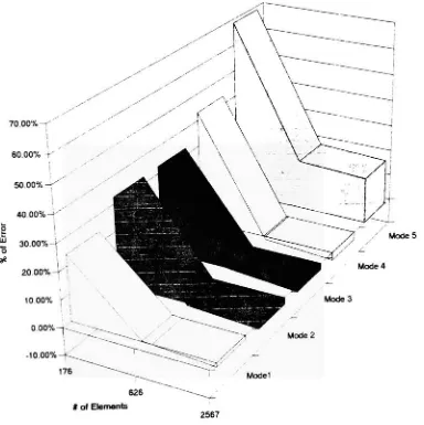
elements.Figure
4.75-4.80 Square flat
plate model and mode1-5
mode shapew/
626 LT
elements.Figure
4.81-4.86 Square
flat
plate model and mode1-5
mode shapew/
2567 LT
elements.Figure 4.87-4.92 Square flat
plate model andmode1-5
mode shapew/
19320
LT
elements.Figure
4.93-4.98 Square flat
platemodel and mode1-5
mode shapew/
Figure 4.99-4.104
Square
flat
plate model and mode1-5
mode shapew/
626 QT
elements.Figure 4.105-4.110 Square
flat
plate model and mode1-5
mode shapew/
2567 QT
elements.Figure 4.111-4.117 Circular flat
plate model and mode1-6
mode shapew/
20
LQ
elements.Figure 4.118-4.124 Circular flat
plate model and mode1-6
mode shapew/
40
LQ
elements.Figure 4.125-4.131 Circular flat
plate model and mode1-6
mode shapew/
100
LQ
elements.Figure 4.132-4.138 Circular flat
plate model and mode1-6
mode shapew/
140
LQ
elements.Figure 4.139-4.145 Circular flat
plate model andmode1-6
mode shapew/
300
LQ
elements.Figure 4.146-4.152 Circular flat
plate model andmode1-6
mode shapew/
600
LQ
elements.Figure 4.153-4.159 Circular flat
plate model and mode1-6
mode shapew/
20
Figure
4.160-4.166
Circular
flat
plate model and mode1-6
mode shapew/
40
Figure
4.167-4.173 Circular
flat
plate model and mode1-6
mode shapew/
80
Figure
174-4.180 Circular flat
plate model and mode1-6
mode shapew/
140
Figure 4.181-4.187
Circular flat
plate model and mode1-6
mode shapew/
600
Figure 4.188-4.194
Circular
flat
plate model and mode1-6
mode shapew/
141 LT
elements.Figure
4.195-4.201
Circular flat
plate model and mode1-6
mode shapew/
209
LT
elements.Figure
4.202-4.208 Circular flat
plate model and mode1-6
mode shapew/
729 LT
elements.Figure 4.209-4.215 Circular
flat
plate model and mode1-6
mode shapew/
2300
LT
elements.Figure 4.216-4.222
Circular
flat
plate model and mode1-6
mode shapew/
16088
LT
elements.Figure
4.223-4.229 Circular flat
plate model and mode1-6
mode shapew/
141
QT
elements.Figure
4.230-4.236 Circular
flat
plate model and mode1-6
mode shapew/
209 QT
elements.Figure
4.237-4.244
Circular
flat
plate model and mode1-6
mode shapew/
729 QT
elements.Figure 4.245-4.251
Circular
flat
plate model andmode1-6
mode shapew/
2300 QT
elements.Page vi
Figure 4.252-4.258
Circular
flat
plate model and mode1-6
mode shape w/3055QT
elements.Figure 4.259-4.265 Circular
flat
plate model and mode1-6
mode shapew/
11021 QT
elements.Figure 6.6 Type
ofelementsFigure 5.1 Cantilever
(square)
beam
#
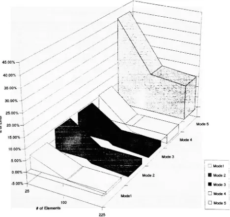
of elements vs.%
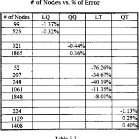
of errorFigure 5.2 Cantilever
(square)
beam
#
of nodes vs.%
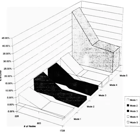
of errorFigure 5.3
Cantilever
(round)
beam
#
of elements vs.%
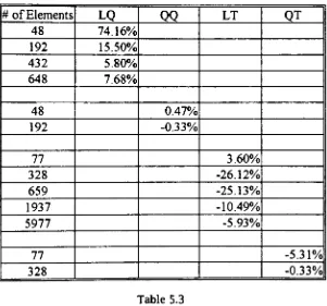
oferrorFigure 5.4 Cantilever
(round)
beam
#
ofnodes vs.%
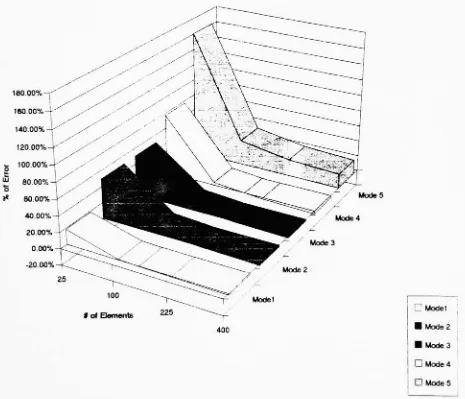
of errorFigure 5.5
LQ
element#
of elements vs.%
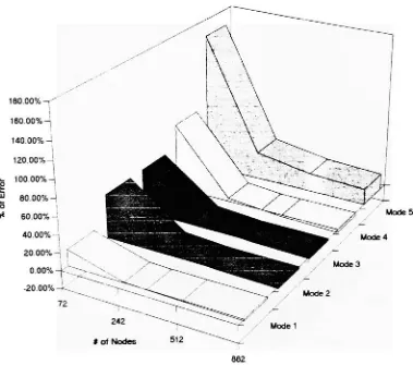
of errorFigure 5.6
LQ
element#
of nodes vs.%
oferrorFigure 5.7
#
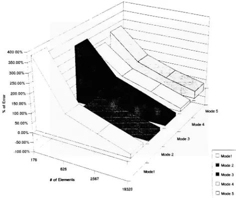
of elements vs.%
of errorFigure 5.8
#
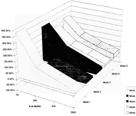
ofnodes vs.%
of errorFigure 5.9 LT
element#
of elements vs.%
of errorFigure 5.10
LT
element#
of nodes vs.%
of errorFigure
5.11
QT
element#
of elements vs.%
of errorFigure 5.12 QT
element#
of nodes vs.%
of errorFigure
5.13
LQ
element#
of elements vs.%
of errorFigure 5.14
LQ
element#
of nodes vs.%
of errorFigure
5.15
#
of elements vs.%
of errorFigure
5.16
#
of nodes vs.%
of errorFigure 5.17
LT
element#
of elements vs.%
of errorFigure 5.18
LT
element#
of nodes vs.%
of errorFigure 5.19 QT
element#
of elements vs.%
of errorFigure
5.20 QT
element#
of nodes vs.%
of errorFigure
6.1
Displacement
of cantilever(square)beam
withLQ
elementsFigure
6.2
Displacement
of cantilever(square)beam
with wedgeelements
Figure
6.3
Displacement
of cantilever(square)beam
with wedge elementsFigure
6.4
Displacement
of cantilever(square)beam
with wedge elementsFigure
6.5
Displacement
of cantilever(square)beam
with wedge elementsFigure
6.6
Type
of elementsFigure
6.7
Mode
1
of circular plate#
of elements vs.%
oferrorFigure
6.8
Mode
1
of circular plate#
of nodes vs.%
oferrorFigure
6.9
Mode
2
of circular plate#
of elementsvs.%
of errorFigure
6.10
Mode
2
of circular plate#
of nodes vs.%
oferrorFigure 6.11
Mode
3
of circular plate#
of elements vs.%
of errorFigure 6.12
Mode
3
of circular plate#
of nodes vs.%
of errorFigure
6.13
Mode
4
of circular plate#
ofelements vs.%
of errorFigure
6.14 Mode 4
of circular plate#
ofnodes vs.%
of errorFigure
6.15 Mode 5
of circular plate#
of elements vs.%
of errorFigure 6.17 Mode 6
ofcircular
plate#
of elementsvs.%
of errorFigure 6.18 Mode 6
of circular plate#
of nodes vs.%
oferrorFigure 7.1
Housing
FEA
results withQT
elementsFigure 7.2
Housing
FEA
results withQT
elementsFigure 7.3
Housing
FEA
results withQT
elementsFigure 7.4
Housing
FEA
results withQT
elementsFigure 7.5
Housing
FEA
results withLT
elementsFigure 7.6
Housing
FEA
resultswithLT
elementsFigure 7.7
Housing
FEA
resultswithLT
elementsFigure 7.8
Housing
FEA
resultswithLT
elementsPageviii
List
ofTables
Table 4.1
#
of elements&
nodesvs.%
of errorTable 4.2 #
ofelements&
nodesvs.%
of errorTable 4.3
#
of elements&
nodesvs.96
of errorTable 4.4 #
of elements&
nodes vs.%
of errorTable 5.1
#
ofelementsvs.%
of errorTable 5.2 #
of nodes vs.%
of errorTable 5.3 #
of elementsvs.%
of errorTable 5.4
#
of nodesvs.%
oferrorTable 5.5
#
of elements&
nodes vs.%
of errorTable 5.6 #
of elements&
nodes vs.%
of errorTable 5.7
#
of elements&
nodes vs.%
of errorTable 5.8
#
of elements&
nodesvs.%
of errorTable 5.9
#
of elements&
nodes vs.%
of errorTable 5.10
#
of elements&
nodes vs.%
of errorTable
5.11 #
of elements&
nodes vs.%
of errorTable 5.12
#
of elements&
nodes vs.%
of errorTable 6.1
Mode
1
of circular plate#
of elements vs.%
of errorTable
6.2
Mode
1
of circular plate#
of nodes vs.%
of errorTable
6.3
Mode
2
of circular plate#
of elements vs.%
of errorTable
6.4
Mode 2
of circular plate#
of nodes vs.%
of errorTable 6.5
Mode
3
of circular plate#
of elements vs.%
of errorTable 6.6
Mode
3
of circular plate#
of nodes vs.%
of errorTable 6.7
Mode 4
of circular plate#
of elements vs.%
of errorTable
6.8
Mode 4
of circular plate#
of nodes vs.%
of errorTable
6.9 Mode 5
of circular plate#
of elements vs.%
of errorChapter
1.
Introduction
The
finite
element methodis
one ofthe
numerical techniques usedfor
the
approximate solution ofengineering
problems.The
proceduresfor FEA
canbe divided
into
three
stages:1.
Pre-processor
2. Processor
3. Post-processor
The Pre-processor
is
the
stageto
makegeometry
(model),
createelements
(mesh)
andapply
the
boundary
conditions.The
processoris
a numerical solver which solvesthe
FEA
model.The
post-processoris
atool
which allowsthe
userto
seethe
results.Once
the
FEA
modelis
finished,
the
user canonly
sendit
to the
solver(processor)
and checkthe
result(post-processor)
afterthat.
The
userhas
no control atthe
processor andthe
post processor stages.The
most critical stageis
the
pre-processor.At
this
stage,
the
user mustfully
understandthe
problem and use allthe tools
which are providedby
the
FEA
program.A
single mistake canadversely
effectthe
FEA
result.If
the
userfully
understandsthe
problem,
the
only
thing
that
canimpede
the
results arethe tools
of pre-processor which are providedby
the
program.Finite
element solvers can give solutionsto
rather complexproblems and
have
traditionally
been
usedfor
analysis ofcomponents with complicated shapes andboundary
conditions(loads
andconstrains).Various
solvers exist which will givereasonably
accurate and reliable resultsfor
these
problems.All
the
finite
element computer packages require aninput
of afinite
elementmesh,
loads,
boundary
conditions(constraints)
and material properties.The
finite
element meshdescribes
to the program, the
discrete geometry
ofthe
domain
to
be
analyzed.Communicating
this
meshto the
finite
element solverhas normally been
done
manually
andthus
has been
time-consuming
and error-prone.The
usefulness ofgeometric modelersfor finite
element mesh generationis readily
apparent.Since
afinite
element meshcommunicates
the
geometry
ofthe
domain
to
be
analyzed, it
seems appropriatethat
it
couldbe
constructedfrom
the
geometry
ofthe
domain in
question.The geometry
of parts and assemblies are stored on computersusing
programs calledgeometric modelers[1,2].
Page
1
Geometric
modelers
The
geometric modelerscanbe
classifiedinto
varioustypes
according
to the
way
they
storethe
geometry
of a object.1)
Wire
frame
modelersThe
objectis
representedby
its
edges.Imagine putting
a wirefor
every
edgein
the
object.The resulting
representationis
a wireframe. No
information is
presentregarding
the
surface.Because
it
does
notcompletely
represent an object with asurface,
it
couldlead
to
an ambiguousobject,
a exampleis
givenin
Figure 1.1.
^^
y
/
/
^s
/s
Toptobottom? Fronttoback?
&
w
Wireframe
Figure 1.1 Wire
frame
representation2)
Surface
modelersThe
objectmay
be
representedby
its
surfaces, curved surfaces canbe
represented and objects are unambiguous.There
is
noinformation
regarding
whatis inside
or outsidethe
object.Thus
it is
not possibleto
computethe
volume or other properties ofthe
object.3)
Solid
modelersThe
objectmay
be
representedin
various waysbut
it is
defined
unambiguously
andit
shouldbe
possibleto
computevolume, mass,
etc.There is
information
regarding
the
inside
and outside ofthe
object.In
ambiguity.
Most
solid modelers storethe
geometry
data in
away
that
canbe
classifiedin
one ofthe three
categories ortheir
combinations.Constructive
Solid
Geometry
(CSG)
The
objectis
built
by
performing
Boolean
operations(union,
difference,
andintersection)
onsimple pre-defined objects calledprimitives,
such asblocks,
cones, cylinders,
tube,
spheres,
etc.The
actualboundary
ofthe
objectis usually
notstoredbut
canbe
computed atany
time.
An
exampleis
givenin Figure 1.2.
Figure 1.2
Constructive Solid
Geometry
modelerBoundary
Representation
(bRep)
The
boundary
ofthe
objectis
storedin
whatis
calledboundary
file
in
a structured manner suchthat
it
is
possibleto
identify
the
regionsinside
or outsidethe
object.The
boundary
ofthe
boundary
ofthe
body
willusually
be
an ordered set ofsurfaces,
faces,
loops
edges and vertices.An
exampleis
givenin Figure 1.3.
Cell
Decomposition's
andSpatial Enumeration
The
objectis
representedby
decomposing
it into
abunch
ofcells,
cubes or
blocks,
which canbe
thought
of asbuilding
up
the
object.The
domain
ofthe
objectsis
representedby
atree
structure,
quadtreein
2-Page
3
dimension
and octreein
3-dimension,
with status ofthe
cells(partial,
full
andempty),
seeFigure 1.4.
for
example.The
boundary
of an objectcan
be
approximatedby
the
cells.Object
Figure
1.3
Boundary
representation modelerThe
early
systemsthat
simply
computerizedthe
drafting
process
do
not contain allthe
geometricinformation
neededto
allow applicationsto
operate automatically.Therefore
,the
more recent solidmodeling
systemsemploy
complete and unique geometricrepresentations.
These
systems contains allthe
geometricinformation
neededto
allowany
finite
element mesh generationtechniques to
automated.Z
1
o
0
Figure
1.4 3-dimensional
octree modelerapplications
to
operate automatically.Therefore
,the
more recent solidmodeling
systemsemploy
complete and uniquegeometricrepresentations.
These
systems contain allthe
geometricinformation
needed
to
allowany
finite
element meshgenerationtechnique to
be
automated.
Approaches
to
mesh
generationThe
problemofmeshgeneration[3]
is
to
convertthe
geometry
from
one ofthe
geometric modelersto
aform
understoodby
afinite
element
solver, in
a manner as automatic as possible.The
increase
in
the
level
of automationwill allowthe
finite
element methodto
be
usedby
engineers
to
provide reliable analysis resultsto their
problem.There
are various popular ways ofgenerating
these
meshes andthey
canbe
classified
into
the
following
categories.1. Laplacian method,
2.
mapping
methods,
3.
point placementfollowed
by
triangulation,
4.
removal ofindividual sub-domain,
5.
recursive subdivision ofthe
domain,
and6.
spatialdecomposition followed
by
subdomain
meshing.An
automatic mesh generatoris
an systematic procedure capableof
producing
a validfinite
element meshin
adomain
ofarbitrary
complexity
given noinput
pastthe
computerized geometricrepresentation of
the
domain
to
be
meshed.The Laplacian
method andmapping
method are notthe
real automatic mesh generationtechniques.
But
both
two
methods arewidely
used(especially
for
quadratic
brick
(Hex)
element orlinear brick
element)
in
the
finite
element method.Laplacian Method
A
set ofsimultaneous nonlinear equationsfor
the
position vectorsof
the
interior
nodes with respectto the
neighboring
nodesis
solvedusing
iterative
techniques.A starting
gridis
required.The
laplacian
methoditeratively
replacesthe
interior
nodePj
Page 5
NJ
Pi
="Pj
Eq. 1.17=1 ;'*i
where
Nj
is
the
number of nodesto
whichPj
is
connected andPj
arethe
nodepoints of
the
connectednodes.The
processhas
proven usefulin
mesh generation algorithms and smoothes
the
meshinto
one withbetter
proportioned elements.
This may
be
usedto
smooth meshes createdusing
other methods.Mapping
Methods
A
function
is
usedto
map
the
givengeometry
into
a simplegeometry,
usually
a squarein
two
dimensions
and a cubein
three
dimensions.
This
simplegeometry is
meshed and allthe
node points aremapped
back
to the
originalgeometry.Various
mapping functions have
been
used, the trans-finite
mapping
are mostcommonly
usedfor
mappedmesh generation.
Mapping
methodsdo
impose
a number of restrictions onthe
geometry
ofthe
object.When
mapping
methods areused,
the
geometry
ofthe
objectis
constructedby
gluing
together the
individual,
fixed
topology,
mesh patches(see Figure 1.5).
Therefore,
the
geometric representationis
explicitly defined
in
terms
of meshpatches.The
useris
responsiblefor
defining
a valid set of meshpatches,
whichimplicitly
define
the
geometric representation andexplicitly
providethe
geometry necessary for meshing
to
occur.The
mesh generatorsare,
therefore,
not concerned withthe
actualgeometry
a.
Body
coordinateb. Mapped
on a unit cubec.
Mesh
generatedof
the
object.This is
however,
notthe
casefor
an automatic meshgenerator which
is
given a complete geometricrepresentationofthe
domain
ofinterest
andis
responsiblefor
decomposing
it
into
a valid set of elements.This
paperwill notdiscuss
this
otherthan to
say
that the
mapping
techniques
have been
found
to
be
ratherinadequate
for
automatically generating
meshes onarbitrary
complex geometry.Automatic Mesh Generation
Techniques
The
other mesh generation methods arefully
automatic mesh generationprocedures,
which arefully
3-dimensional
orthe
extensionfrom
2-dimensional
to
3-dimensional
mesh generation appears possible.Currently,
these
mesh generationtechniques
only
use tetrahedron elementsin
3-dimension;
no othertype
of elements are available.1. Point
placementfollowed
by
domain
triangulation
This
type
of mesh generatorinvolves
two
independent
process[6,7,8,9].
First,
node points mustbe
inserted
within and onthe
boundary
of
the
structureto
be
meshed.Secondly,
the
node points areautomatically
triangulated to
form
a network of well-proportioned elements.The
triangulated
algorithmsfunction
in
both
2- and3-dimensional
settingsproducing
meshes oftriangular
andtetrahedral
elements,
respectively.These
two
algorithmsfunction
independently
of eachother,
sothat there
aremany
waysto triangulate
the
elements.For
ease of
exposition,
wefirst discuss
a meshtriangulation
algorithm.Recent
efforts[6,10,11,12]
employ
the
properties ofthe
geometricconstructs of
Dirichlet
tessellation
and moreimportantly
for
meshgeneration, the
Delaunay
triangulation
of given set of points, considerfirst
the
2-dimensional
case.Let
Pj,
P2,...,Pn
be distinct
pointsin
the
plane,
anddefine
the
setsVi(
l<i<N,
whereVr{X:
IX-Pil
<IX-Pjl
for
allj*i}
Eq. 1.2
where
|.|
denotes
Euclidean
distance
in
the
plane.Vj
represents aregion ofthe
planewhose points are nearerto
nodePj
than to
any
other nodes.Thus
Vj
is
an open convex polygon(usually
called aVoronoi
polygon)
whoseboundaries
are portions ofthe
perpendicularbisectors
ofthe
lines
joining
nodePj
to
nodePj
when%
andVj
are contiguous.The
collection of
Voronoi
polygonsis
calledthe
Dirichlet
tessellation.
In
general,
a vertex of aVoronoi
polygonis
sharedby
two
other polygons soPage
7
that
connecting
the
three
generating
points associated with suchadjacent polygons
form
atriangle,
say T^.
This
set oftriangles
n_}
is
calledthe
Delaunay
Triangulation. See
Figure
1.6
for
example.Figure 1.6 Dirichlettessellationand
Delaunay
triangulationThe
construct canbe
shownto
be
atriangulation
ofthe
convexhull
ofthe
node points.An
important
property
of2-dimensional
Delaunay
Triangulation
which makesit
suitablefor
use as afinite
elementthat
its
triangles
are as close or equilateral as possiblefor
the
given set ofnodes.Consequently,
ill-conditioned
andthin triangles
are avoided whenever possible.There
aremany
approachesto the
construction of a
Delaunay
triangulation.
A currently
popular approachis
a version proposedby
Watson[8].
In
two
dimensions,
Watson's
algorithmturns
uponthe
simpleobservation
that three
given node points willform
aDelaunay
triangle
if
and
only
if
the
circumdiskdefined
by
these
nodes contains no other node pointsin
its interior.
The
algorithmis
initialized
by
calculating
the
coordinates ofthree
nodepoints whichform
atriangle
Tq
that
surrounds all
the
node pointsto
be
inserted. The
circumcentrecoordinates and circumradius of
the
circumcircledefined
by
T0
are also calculated and recorded.The
node points arethen
introduced
one at atime.
The
algorithm operatesby
maintaining
alist
oftriplets
of node points which represent completedDelaunay
triangles.
Associated
with each suchtriangles
arethe
coordinates ofits
circumcentre andcircumradius.
For
each new nodepointentered,
a searchis
made ofall currenttriangles to
identify
those
whose circumdisks containthe
new point.For
suchdisks,
the
associatedtriangles
areflagged
to
indicate
removal.
As
shownin Figure
1.7,
the
union of all suchtriangles
forms
be
shownthat
nopreviously inserted
nodeis
containedin
the
interior
ofthe
polygon andthat
eachboundary
node ofthe
polygonmay
be
connected
to the
new nodeby
astraightline
lying
entirely
withinthe
polygon.Thus,
a newtriangulation
ofthe
region enclosedby
the
polygonis
formed.
Repeated
use ofthis
insertion
algorithm permits all nodepoints
to
be
entered,
while ensuresthat
at eachstep
the
triangulation retainsits
Delaunay
properties.a.
New
pointinsertion
b.
Element deletion
c.New
mesh generatedFigure 1.7 Watson's Algorithm
In
three
dimensions,
Watson's Algorithm
starts with atetrahedron
To
containing
all pointsto
be
inserted,
and newinternal
tetrahedron
areformed
asthe
points are entered one at atime.
At
atypical
stage ofthe
process,
a new pointis
tested to
determine
which circumspheres ofthe
existing
tetrahedron
containsthe
point.The
associatedtetrahedra
areremoved,
leaving
aninsertion
polyhedroncontaining
the
new point.Edges connecting
the
new pointto
alltriangular
faces
ofthe
surface ofthe
insertion
polyhedron arecreated,
defining
tetrahedral
whichfill
the
insertion
polyhedron.Combining
these
withthe
tetrahedral
outsidethe
insertion
polyhedron produces a newDelaunay
triangulation
whichcontains
the
newly
added point.There
are a number of waysthat
node points canbe
inserted
within
the
domain. For
instance,
one ofthese
methods usedin
[6]
is
to
cut planesthrough the structure,
say P1,P2,...,Pn. It
is
within each ofthese
cross-sectionsthat
nodepoints willbe defined.
Figure
1.8
illustrates
the
stepsto
define
the
node pointsin
a space.In
summary
,node points are
defined
interactively
aplane-at-a-time.Within
eachplane, the
userhas
control overlocal
nodedensities.
It is
possibleto
automatethis
nodeinsertion
processfurther.
Page
9
Figure
1.8
A waytodefine
thenodepointsinspaceAlthough
Delaunay
triangulation
performsvery
wellin
two
dimensions,
several problems exist withWatson's
approachin 3-D.
The
first
oneis
the
existence ofdegenerate
cases.These
occurin
practicewhen a
newly inserted
node appearsto
he
onthe
surface of acircumsphere associated with some
existing
tetrahedron.The
problembecomes
apparent wheneverthe
distance from
anewly
enterednodalpoint
to
anexisting
circumsphereis less
than
e,
where eis
the
expectedaccumulated computer
truncation
error.This in
turn
producesstructural
inconsistencies in
the
triangulation,
that
is
overlapping
tetrahedral
orgap
in
the
mesh.Delaunay
tedrahdron
circumsphere
Figure 1.9 The
distorted
Delaunay
tetrahedron,
"silver"Another
serious problem which arisesin
the three
dimensions,
and which also requires modification of
the
Delaunay Triangulation,
occurs with
the
creation oftetrahedron
we call"silver".
In
this
case(see
Figure
1.9),
"silver"
will
defines
abadly
distorted
Delaunay
tetrahedron
made
arbitrary
small.Therefore,
these
methods which useDelaunay
Triangulation
needchecking
criterionto
eliminatethose
ill-shaped
elements after
the
mesh elementshave been
generated.i
-_--->
4.1
!
Figure
1.10
Surrounding
algorithmOther
rule-based procedures oftriangulation
have been developed
[7,8].
For
instance,
in
two
dimensions,
a methodbinges
onthe
principle offully
surrounded points.Starting
with node1,
each nodeis
surrounded
in
turn
withtriangular
elements.When
a nodeis
being
surrounded,
newtriangles
areonly formed
with nodes ofhigher
node number whichis
registeredby
a specialscanning
procedure.This
automatically
ensuresthat
triangles
do
not overlap.The
process startsby
selecting
the
nearestpoint
to
node1
andthus
estabkshing
a sidelj
wherej
is
the
nodenumber of
the
nearest point.When surrounding
another pointi,
the
first
side
is
establishedonly
afterchecking
whetheri is
already
part of anexisting
triangle.If
this
is
the
case,
the
existing
triangle
is
usedto
provide
this
starting
side.The
sideij
is
then
usedto
seek a nodek
suchthat the
anglei-k-j
is
maximum andi-j-k is
an anti clockwise sequence.This
new pointk
becomes
j
andthe
processis
repeated and so on.If
a node1
is
found
suchthat
triangle
ikl already
existsthis
routineis
omitted and
1
becomes
the
new pointi.
The
process stopswhen atriangle
is
obtainedcontaining
the
sidefrom
whichthe
processbegan
and
the
pointis
thus
completely
surrounded(see Figure
1.10
for
detail.)
The
extensionto
3-dimension
couldbe in
[9].
In
this
approach,
the
surrounding
a given point withtriangular
elementis
replaced withsurrounding
aline between
two
points with elements andthen
move onto
anotherline
untilthe
meshis
complete.A
flow
chart ofthis
routineis
shown
in
Figure 1.11.
Page
llSTART
Determingtheline
tobesurrounded[1-2]
Determingthebasic
triangle[1-2-3]
<r
Lookingfortheoptimum point[4]andformingthe the tetrahedron[1-2-3-4]
>1
|3]=[4]
End
=Surroundingangle
Figure 1.11 The flow chart ofthe
3-dimensional
surroundingalgorithmThe
nodeinsertion
ofthe
surrounding
algorithm mentioned above usesa
slightly
different
scheme.The
node point numberis
recordedin
sequence
by
a specificscanning
procedure.When
allthe
"true" node pointshave
been
recorded, the
number ofthe
last
nodeis
noted andthen
startto
record"ghost"
points outside
the
boundaries
ofthe
structure,
seeFigure 1.12
The
use of"ghost"
points removes
the
needfor
the
identification
ofnodes on externalboundaries.
Ghost
points mustbe
placed so
that
each element side whichis
on an externalboundary
canform
atriangle
with a ghost point.Otherwise,
the
mesh generationprogram will
form
atriangle
whichdoes
not exist onthe
structurebetween
the
boundary
node points.These
"ghost"
triangles
willbe
removed after
the
mesheshave
been
generated.Though
these
algorithms useproperly
constructed set of rulescapable of
producing
a well-conditioned meshwithin adomain,
they
require extensivesearching
andlarge
number ofchecks,
suchasdegenerate
andoverlapping
cases,
many
morethan
other meshtriangulation
rulesthat
wouldinsure
the
elements generatedsatisfy
a givenshape criterion.Ghost
points
/
Figure
1.12The
"Ghost"pointfor
boundary
definition
2. Mesh
generationbased
onSub-domain
removalAutomatic
mesh generation proceduresin
this
method[13,14,15,
16]
operateby
removing
individual
piecesfrom
the
domain
one at atime
until
the
domain
is
reducedto
oneremaining
acceptable piece.Element
removal
meshing
proceduresemploy
a specific set of element removal operatorsthat
are capable ofremoving
a single elementfrom
anobject.They
operateby
first examining
the topological
features
ofthe
objecttesting
a specific set of geometric measuresto
seeif
any
ofthe
element removal operators canbe
applied.There is
a pre-specifiedhierarchy
in
which
the
various operators are applied.They
typically
employ
aboundary
representation ofthe
domain
and operateby
searching for
entities of specifictype that
satisfy
a set ofconductivity
and geometricrequirements.
Two
examples ofthis
kind
are represented asfollowed.
Figure
1.13
Subdivisionof a multilateraldomain
The
first
approachis
an subdivision ofaplanar polygonby
triangular
elements[13].
Given
a certaindomain
with a number of nodes Page13
around
its
boundary,
we startby deterrmning
the
most well-conditionedelements which can
be
formed
at each corner ofthe
domain.
Having
finished
this
step,
the
elementsformed
are consideredto
be
cut outfrom
the
original area andthe
same conceptis
appliedto the
remaining
area and so on.
The
level
equals unity.Subdivision
at a corner node oflevel
equalsunity
generates nodes oflevel
equalsto two
and so on.The
subdivision
ofdomain
is
performed
in
successive stages.In
eachstage,
A
continuous
boundary
layers
is
cut out.This is
shown(Ungrammatically
in
Figure 1.13 & 1.14.
Starting
withthe
nodes aroundthe
originalboundary,
Triangular
elements are generated anda new set of nodes oflevel
equalstwo
are obtained.The
first
stageis
known
to
be
completewhen all
the
nodesbounding
the
areato
be
subdividedbecome
oflevel
equals
two.
Again,
starting
withthese
nodes,
a new set of nodes oflevel
equalsthree
are generatedand so on.The
mesh generation processis
known
to
be
complete whenthe
number of nodes aroundthe
boundary
of
the
remaining
area reachthree.
This
meansthat the
remaining
areais
one single
triangular
element andhence
no more subdivisionis
required.
Contour |
Figure
1.14.
Nodallevels
The
second approach[14]
is
a3-dimensional
subdivision ofobjectwhich
is
extendedfrom
an2-dimensional
procedure.Consider
the
basic
element removal operators used
to
mesh a3-dimensional
subdivisiondomain
without void.The first
operator,
VERTEX_REMOVAL
is
appliedby
searching
the
objectfor
verticeswithonly
three
edgescoming into it.
Any
such vertex satisfies a set of geometricinterference
requirements
canbe validly
removedfrom
the
object.The
removal ofvertex carves atetrahedron
from
the
object.In
cases where allverticeshave
morethan
three
vertices,
a secondoperator,
EDGE_REMOVAL,
is
applied.In
this
case,
tetrahedron
containing
the
selected edgeis
carvedfrom
the
object.the
verticesby
oneofeach,
it
eventually
reducesthe
complexity
ofthe
object untilthe
first
operator canbe
applied again.In
case where neither ofthe
first
two
operators canbe
appliedathird operator,
FACE_REMOVAL,
canbe
applied.In
this
case,
a tetrahedroncontaining
aface
ofthe
object andconnecting
the three
verticesthat
bound
the
face
being
removed.These
operators areillustrated
in
the
Figure 1.15.
(A) VERTEXJIEMOVAL
(B)
EDGE_REMOVAL(C)
FACE_REMOVALFigure 1.15
Elementremoval operatorsA
topological-based
elementby
element removal procedureappears
ideally
suitedfor
the
construction of optimalh-p
(
HEX
element)
finite
element meshes wherecoarse,
exponentially
graded meshes aredesired. Since
the
amount ofcomputationrequiredfor
the
application of each removal operationis
high,
these
procedures are notcomputationally
efficientfor
the
creation of afine
mesh.The
development
of an algorithmthat
decomposes
the
domain
into
large
chunks
by
removing
them
one at atime
is
an attractiveway
to
considerthe
automation ofthe
current methods of mesh generation wherethe
user
interactively
decomposes
the
domain
ofinterest into
mappable regions andinvokes
amapping
mesh generator which wehave
mentioned at
the
beginning
[4,5].
The
difficulty
in
developing
such an approachis
the
identification
andimplementation
of a set of rulesthat
would examine a
geometry
to
determine how
to
decompose
it into
mappable regions
that
will yieldthe type
of mesh generationsdesired
aswell as
providing
asatisfactory
meshtopology.
3.
Mesh
generationby
recursive subdivisionThe
recursive subdivision mesh generators[17,18,19]
operateby
the
repeatedsplitting
ofadomain
into
simplerparts untilthe
individual
parts are single
elements, or,
possibly,
simple regionsin
which elements canbe quickly
generated.The Triquamesh
technique
is
one ofthe
wide used recursive subdivision methodin
this
area.The
Triquamesh
technique
is based
onthe
surface/volumetriangulation.
It
canbe
usedto
create
triangular
or quadrilateralmeshes on surface.It
can alsobe
broken
up
into hexahedrons.
The
wholetechnique
is
based
ontwo
basic
laws
of analyticgeometry
atthis time:
Page
15
Every
polygonis
divisible
into
triangles.
Every
polyhedronis
divisible
into
tetrahedron.
It
follows
that
we willbe
ableto
create a meshconsisting
oftriangles
ofany
surface.Also,
wewillbe
ableto
create a meshconsisting
oftetrahedral
in any
volume.To
explainthe
working
ofthis
method,
we startwith adescription
in
2-dimensions [18].
The
extensionto
3-dimension
is
then
straightforward.
Any
area canbe divided
by
the
userinto
a certain number ofsub-area.
Each
sub-areaneedsto
be
coherent,
that
is,
a closedloop. An
area with n-foldincoherence
canbe
made coherentby
n-1 cuts.The
first step
involves obtaining
a convex polygon.So,
if
the
polygonis already
convex,
we moveto the
next step.Otherwise,
This
polygonis
successively
subdivided,
until abunch
of convex polygons are obtained.This
process ofsubdividing
a concave polygoninto
morethan
one convex polygonsis
controlledby
certainheuristics,
whichhave
essentially been
obtainedby
trial
and error.The
aimis
to
get a splitline
which will passthrough
aconcavity
in
the
concave polygon and whichis
likely
to
yield good elements.These
splitlines have
to
be
chosen rathercarefully because
these
later
become
the
boundaries
ofthe
elements.Once
a polygonis
divided
into
two
by
using
a splitline,
seeFigure
1.16,
we needto
createnodes on
the
splitlines.
The
problem now reducesto
meshing
two
polygons.
This
processis
continued aslong
as wehave
polygons.Once
we
have
convexpolygons,
they
aretaken
up
oneby
one.An
attemptis
madeto
chop
offlayers from
the
polygon,
wherethe
polygonhas
asharp
angle.These
layers
yield elements.These
layers
are choppedsuccessively,
suchthat
each ofthe
layers
yields good elements.Again,
this
is
done using
certainheuristics. Once
no moresharp
corners arefound,
the
polygonis
again cutinto
two
by
use of a splitline
asplitline
Figure 1.16
Cutting
concave polygonusingsplitting line
Figure 1.17 chopping
offlayers
yield elementsThe
same concepts are extendedto
3-dimension A
surfacein
3-dimension
is
projected(or transformed)
to
2-dimension
andthe
abovemeshing is
done.
For
solidelements, tetrahedron
are generated.These
can
later be
subdividedinto
hexahedrons.
We
will nowbe
dealing
withconvex polyhedra
instead
ofpolygons and split planesinstead
of splitlines
then
same proceduresfrom 2-dimensional
meshapplied untilthe
mesh complete.
As in
the
sub-domain removalprocedures,
this
class of meshgenerator
typically
operates off aboundary
representationofthe
domain
to
be
meshed,
looking
for
candidatetopological
features
meeting
specificconductivity
and geometric requirements.Some
structures whichthis
method cannot split shouldbe
transformed
or sub-dividedto those that
can
be
split.4. Spatial
decomposition
followed
by
sub-domainmeshing
The
basic
idea
behind
this
approach[10,11,14,19,20,21,22,23]
is
use an efficient procedure
to
decompose,
in
acontrolledmanner,
the
domain
ofinterest
into
a set of simple cells andto then
meshthe
individual
cellsin
sucha mannerthat the
resulting
meshis
valid.The
one spatial
decomposition
approachthat
has been
appliedto
meshgeneration
is
the
quadtreein
2-dimensions
andthe
octreein
3-dimensions. The
entire structureis
storedin
ahierarchic
tree
as shownin
figure
1.18.
One
algorithmto
building
a3 dimensional
meshgeneratorusing
this
basic
tree
representationis
the
modified-octree(modified-quadtree
in
2-dimension)
[21,22,23].
the
basic
stepsin
the
modified-octree meshgenerating
processes are :a.
Set
up
aninteger
coordinate systemthat
containsthe
objectto
be
meshed.Page 17
b.
Generate
the modified-octree
representation ofthe
objectaccounting
for
the
mesh gradationinformation
specified withthe
geometricmodel.
c.
Break
the modified-octree
up into
avalidfinite
element mesh.d.
Pull
the
nodes onthe
boundary
ofthe
modified-octreeto the
appropriate
vertices,
edges andfaces
ofthe
original geometry.e.
Smooth
the
locations
ofthe
node pointsto
create abetter
conditioned
finite
element mesh.iff
%
m
%
m s_r QUADTREEREPRESENTATIONTOP FOUR
LEVELS
OFTREE
FULL
EMPTY
PARTIAL
MOOlflEO
OUAOTREE
REPRESENTATION
Figure 1.18 Thequadtree and modified quadtree representations
The
essentialdifference
between
an octree and amodified-octree
is
that the
modified-octree allowsfor
the
definition
of a cut octant.Since
the
size of octree cubesdesired for
usein
the
finite
element meshgeneration are
large
with respectto the
geometricdetails
ofthe
object, it
is necessary
to
deal
in
a specific manner withthose
octree cubesthat
containthe
boundary
ofthe
object and are neitherfully
inside
nor outsidethe
object.The
cutoctants,
whichis
the
octantscontaining
the
boundary
ofthe object,
is
completedby
qualifying
which side ofthe
discrete
boundary
existing
in
the
octantis inside
the
object.To
maintainthe
integer
tree
storage andto
limit
the
number of cutoctant casesto
amanageable
number,
only
the
corners andhalf-points
ofan octant casesare used
in
the
cutting
process.This
operationrequires a specific set of geometric checks[23].
With
IN/OUT information
ofthese
points,
the
sharp
offaces
ofthe
octantthat
are cutby
the
cutting
surface aredefined. One
approachto
define
the
cutting
surfaceis
to
allowonly
when
the
cutting
surfacepoints
arenot coplanar.In
these
situations,
the
surface
representation
willhave
adiscontinuity,
which willlead
to
problems when
the
final
mesh modifications are performed.Therefore,
it
is
necessary
to
include
amore extensive set of octantcutting
surfaces.The IN/OUT
information
canbe
properly
represented with an addition of a set oftwo
planar cut octants andalimited
number ofthree
planarcuts,
seeFigure 1.19. After
the
octant onthe
boundary
aredefined,
the
interior
octants withinthe
boundary
arethen
quickly filled
by
a simpletree traversal
process.
Once
the
modified-octreeis
available,
it is broken
into
a set of validfinite
elements.After
aninteger
finite
element meshis
available,
the
final
stepsinclude pulling (or
assign)
nodesto the
boundary
andsmoothing
the
nodallocations
to
ensurethe
best
possible element sharpsfor
the
given elementtopology.
One
planar cut octant examples
Two
planar
cut octant examples
Figure 1.19 Examplesofcut octants usedinthemodified octree algorithm
Another
approachbased
onspatialdecomposition
usesthe
combination of
Octree
andDelaunay
Triangulation
[10,11,12].
The
basis
of
the
scheme areintroduced
briefly
asfollows
(see
figure
1.20
for
details):
a.
Tree building. Given
a geometricmodel,
generateits
octreerepresentation.
Each
octantis
classifiedinside,
outside,
or onthe
boundary
ofthe
object.An
octantis
classified onthe
boundary
whenany
ofits
features
(vertices,
edges,
orfaces)
is
classified on orintersects
the
boundary.
b.
Octree
triangulation.Each
octant classifiedinside
or onthe
boundary
is
triangulated
using
templates
orDelaunay
procedure.c.
Intersection
point triangulation.The
octreetriangulation
serves asthe
initial
triangulationfor
the
intersection
pointtriangulation
.In
Page
19
this
step
the
intersection
points
generatedduring
tree
building
areincorporated into
the
triangulation using
the
Delaunay
property.Classification
and compatibility.The
geometrictriangulation
requiresthat
the
mesh entities are classified againstthe
modelgeometry
andthat topological
compatibility is
assured.If
anincompatibility
is
identified,
it
resolved eitherthrough
alocal
resolution procedure orby
refining
the
octree.Mesh
improvements.
A
point repositionprocedure,
such asLaplacian
method, may
be
usedto
improve
the
quality
ofthe
mesh elements.Rg
_:?"^
\\
\y*OriginalGeometry TreeBuilding Octreetriangulation Intersectionpoints Classification& Triangulation Comparability
Figure
1.20 A
overview ofoctree/DelaunaytriangulationmethodControl
ofthe
elementdistribution
In
additionto the
ability
to
generate a valid meshfor any
geometry,
automatic mesh generators must permitthe types
of mesh gradationsnecessary
to
produce efficientfinite
element models.Ideally,
the
mesh controldevice
should allowfor
the
convenient specification ofboth
a priori and a posterior mesh generationinformation.
A
priorimesh control
device
are usedto
specify
the
distribution
of elementsin
the
initial
finite
element model.Since
the
basic
input
to
an automaticmesh generator
is
a geometricrepresentation.,
any
priori mesh controldevice
mustbe
tied to the
geometric representation.This
meansthat
apriori mesh control can also
be
afunction
ofthe
particular geometricmodeling
approach used.A
posterior mesh controldevices
are used an adaptive analysis processto
improve
the
mesh asindicated
by
the
resultson
the
overalldiscretization
errorin
one or more solution norms.The
primary function
of a posterior error estimators areto
provide aconvergent and accurate measure of
the
discretization
error of agivenfinite
element solution.To
used mosteffectively, the
mesh generationprocedures must
be
coupledwith adaptive analysisprocedurethat
caninsure that the
final
mesh yieldsthe
requesteddegree
of accuracy.Without
adaptive analysisproceduresbased
on reliable aposterior errorestimators, the
analyst will needto
use a priori mesh controltechniques
Chapter
2. Test Cases
The
benchmark
is
based
ontwo types
of analyses(static
state andmodal
analysis).
Each
type
of analysis willgiventwo
geometries andmeshes
by
linear
and quadratictetrahedron
and quadrilateral elements.All
the
FEA
results willbe
comparedwithhand
calculation.Static State
Cantilever
(square)
beam
1000 lbf
10"xl"xl"
Material :Steel E= 3e7psi u =
.3
Figure2.1
Cantilver
(round)
beam
1000 lbf
D=1",L=10"
Material:Steel - E= 3e7psi u =
.3
Figure 2.2
Page 21
Modal Analysis
Square
flat
plate all edgesfixed
10"
x
10"
x
0.5"
Material :Steel - E= 3e7psiu = .3 Figure2.3
All edgesfixed
Circular
flat
plate with a edgefixed
Edges fixed
OD
= 10"t = 0.5"
Chapter 3.
Analytical Solutions
Cantilever
(square)
beam
smmmmmm
;'-;.>:";"-'::*':-"'a";v" :;"
::: ';'':-::;
1000 lbf
10"
x
1"
x
1"
Material:Steel
-E= 3e7psi o =
.3
Figure3.1
I
=-- =-- =0.08333
in* Eq.3.112
12
37
lOOO(lO)3
3H
= -0.1333
in
Eq. 3.2Page
23
Cantilver
(round)
beam
:^:v^^^^->^ -^ '^A^^^^^^v.^^^s\^^^^^s<^s^^^'.^<;";^^s^^<s^^<^^^W;^...,
;^;->X^:^: -^^^^v^v.^^^^^^^^^^^^^v^A^^^<sW^6^^^s^s^Ww^S^^^^v..,
^^:^^^^^:>- ^^^^^^^^^^^^v.^v.-.^^^^^^<^.^W:0^<4s^vvl.^^ss.,
'^^^^^^^^;-^-^^^^.^^^v^.,.iA^^^.^^^^s^v^.v^.^^*-^v.X<.vA^^^y^v^^^X^.^^J^^v.,
....-...v.s.