The Remaining Useful Life Estimation of Lithium-ion Battery Based on Improved Extreme Learning Machine Algorithm

Int. J. Electrochem. Sci., 13 (2018) 4991 – 5004, doi: 10.20964/2018.05.84

International Journal of

ELECTROCHEMICAL

SCIENCE

The Remaining Useful Life Estimation of Lithium-ion Battery

Based on Improved Extreme Learning Machine Algorithm

Jing Yang1,2,3, Zhen Peng4,Hongmin Wang1,2,3,Huimei Yuan1,2,3, Lifeng Wu1,2,3*

1

College of Information Engineering, Capital Normal University, Beijing 100048, China;

2

Beijing Key Laboratory of Electronic System Reliability Technology, Capital Normal University, Beijing 100048, China

3

Beijing Advanced Innovation Center for Imaging Technology, Capital Normal University, Beijing 100048, China

4

Information Management Department, Beijing Institute of Petrochemical Technology, Beijing 10217, China

*

E-mail: [email protected]

Received: 31 January 2018 / Accepted: 11 March 2018 / Published: 10 April 2018

In order to predict the remaining useful life (RUL) of lithium-ion battery more accurately, a new prediction method based on extreme learning machine (ELM) is proposed in this paper. First, according to the mutation idea of genetic algorithm (GA), we add mutation factors to improve particle swarm optimization (PSO) algorithm. Then, the particles generated by the improved PSO algorithm are used as the input weights and bias of the ELM algorithm. The optimized ELM prediction model is applied to estimate the RUL of the lithium-ion battery. Three sets of data are used to verify the accuracy of the proposed algorithm in this paper.

Keywords: Lithium-ion battery; RUL; ELM; PSO; Mutation factor

1. INTRODUCTION

ape-like robot RoboSimian was in charge of a project. The lithium-ion battery exploded and the whole robot was destroyed.

In order to avoid unnecessary losses, it is necessary to propose the battery management system (BMS), which can effectively monitor the battery pack, accurately estimate the remaining battery pack capacity, and effectively prevent battery safety accidents [4]. The RUL is an important performance indicator of BMS. The battery life is expressed as the cycles of charging and discharging. The battery capacity falls to the threshold (usually 70%-80% of the battery capacity), indicating the end of battery life [5].

The common RUL prediction methods are divided into two categories: model-based prognostics methods and data-driven based methods [6]. Model-based prediction is a mathematical model with physical rules that can reflect the degradation of system performance from the internal working mechanism of lithium-ion batteries [7]. In [8], the battery capacity of lithium-ion batteries is estimated based on extended kalman filtering (EKF) method, which is compared with other prediction methods to prove the effectiveness of the method. The literature [9] improves the particle filter (PF) algorithm with the artificial fish swarm algorithm. The improved PF algorithm is used to predict the remaining useful life of the lithium-ion battery. However, due to the complicated internal characteristics of lithium-ion batteries, it’s complex and difficult to achieve model-driven method [10-11]. Data-driven approach can effectively avoid these shortcomings by monitoring the state of the system, analyzing the state behavior of the analyzer according to historical data and converting it into relevant models to predict the future state of the system [12]. These approaches have been applied to predict the RUL of lithium-ion battery [13-17]. Support vector machine (SVM) is one of the model-based methods. The literature [18] first extracts the characteristics of the temperature and voltage, then uses the SVM method to predict the RUL, and has achieved good results. However, SVM has high computational complexity and consumes computational time in practical applications. The relevance vector machine (RVM) method is based on the SVM method, which reduces the computational complexity. In [19], wavelet denoising method is used to improve the certainty of RVM method, and a time series prediction model is constructed, which achieves good results for battery life prediction. However, the high degree of sparsity of the RVM approach determines the output instability of its results. The Artificial Neural Network (ANN) has the advantages of flexibility and easy implementation [20], and has been applied to the prediction of the remaining useful life of lithium-ion batteries. In [21], the author predicted the RUL of lithium-ion batteries by ANN method and traditional method. The results show that the ANN method is more effective. In [22], BP neural network is used to predict battery capacity and achieved good results. However, artificial neural networks also have some disadvantages such as long training time and complex calculation.

mobile lithium batteries. In [27], an indirect prediction model of ELM is used to estimate the RUL based on the novel heahth indicator (HI). [28] proposes the online sequential ELM (OS-ELM) prediction model and uses the indirect method to predict the SOC of the lithium battery. In [29], ELM is used to predict the RUL.

The ELM method will greatly reduce the training time, but at the same time, its prediction performance will be affected. In this paper, the weights and bias in ELM are optimized. According to the principle of mutation in GA, particle swarm optimization (PSO) algorithm is improved and forms mutation particle swarm optimization (MPSO) algorithm, which has better optimization ability to optimize the weights and bias of ELM. In this paper, NASA’s lithium-ion battery data sets are used and the experiment results show that the prediction error of the proposed method is smaller.

The structure of this paper is as follows: the second part briefly introduces the techniques, algorithms and methods, including ELM and PSO. The third part is about the experiments. The proposed method compared with the other algorithms is discussed in fourth part. The conclusion is drawn in fifth part.

2. METHODS OUTLINED 2.1. Extreme learning machine

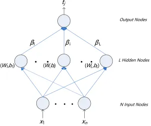
ELM is a single hidden layer neural network, including the input layer, hidden layer and output layer, as shown in Fig.1, X1, X2, …, Xn are input variables of the network, W1, W2, ..., WL are input

weights, b1, b2, ..., bL are bias and the output value is tj [30].

Output Nodes

L Hidden Nodes

N Input Nodes

β1 β i β L

(W1 ,b1 ) (Wi ,bi ) (WL ,bL )

x1 xn

tj

The ELM algorithm procedures [23] are as follows:

(1) Randomly generate input weight vectors [W1, W2, …, WL] and bias[b1, b2, …, bL],

where L is the number of hidden nodes.

(2) Determine the formula and the activation function. According to the calculation formula of neural network, the relation between its input and output is as follows:

(1) where G(x) is the activation function; Eq.(1) can be written as follows:

(2) in which,

(3) (3) Calculate the output weight. The value of the generalized inverse matrix β is calculated by the Eq.(2)

(4) H+ is the Moore-Penrose generalized inverse of H.

From the ELM algorithm steps, it can be seen that compared with the traditional neural network, the ELM algorithm has no iterative steps, thus greatly reducing the training time and computational complexity.

2.2. MSPO

PSO algorithm belongs to the group intelligent optimization algorithm [31]. It is a population-based algorithm. In a space, a group of particles is initialized, and the particle's characteristics are represented by three indicators: location, speed and fitness. [32]. The performance of each particle is measured by the fitness function. Particles move at a certain speed and update their positions in multidimensional space, and the fitness of particles is calculated every time they are updated [33].

In a M-dimensional space, there are n particles which make up the population X= (X1, X2,...Xn),

Xi represents the position of the ith particle in space, which is also a potential solution [34]. According

to the objective function, the fitness value corresponding to each particle position Xi can be calculated.

Pi= [Pi1, Pi2, ...,PiM] represents the individual extreme value, and the global extreme value of the

population is Pg = [Pg1, Pg2, ..., PgM]. In each iteration, the particle updates its velocity and position

according to the individual extremum and the global extremum [35]. The update formulas are: (5) (6) where the inertia weight is represented by ω, d = 1,2, ..., M, i = 1,2, ..., n. k is the number of current iterations. Vid is the particle velocity. c1 and c2 are the acceleration factors and are non-negative

constants. r1 and r2 are random numbers whose values are distributed between [0, 1]. The general

However, PSO algorithm has some shortcomings: low iteration efficiency and the possibility of not getting the global optimal solution. Literature [36] proposed the MPSO, which is based on the idea of adaptive operation of genetic algorithm, some variables are reinitialized with a certain probability, so as to improve the PSO algorithm. The mutation operations extend the ever-narrowing population search space in iterations so that particles can jump out of the previously found optimal value positions. Therefore, based on the PSO algorithm, a simple mutation operator is introduced. The basic idea is that after each particle update, the particle is reinitialized with a certain probability, and the improved algorithm has better performance. The steps of MPSO are as follows:

Algorithm 1. PSO algorithm Step1. Initializing particles and velocities;

Step2. Finding the optimal value of individuals and the optimal value of population; Step3. Updating the particles and speed;

Step4. Adaptive mutation; Step5. Estimating fitness function;

Step6. Updating individual extreme value and global extreme value; Step7. Determining whether to meet the conditions, if not satisfied, and then go to

Step3, otherwise, to generate particles.

2.3 MPSO-ELM algorithm

Data

Train Data Test Data

Train Output Data Train Input Data Test Input Data Test Output Data

Training ELM Initializing

particles and velocity

Fitness

Evaluation Mean Square Error

Trained ELM

Predicted Result Find Fitness

Value

Updating particles and

velocity

Adaptive mutation

Updating Fitness Value

Input weights and bias

Meet end conditon? NO

YES

Evaluate

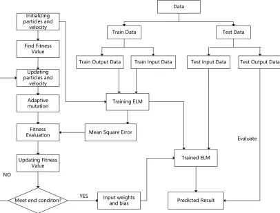
From the first step of ELM algorithm, we know that the input weights and bias of ELM algorithm are randomly generated, although the training time is greatly reduced, its accuracy will also be affected. In this paper, an improved MPSO-ELM method is proposed to optimize the input weights and bias of the ELM algorithm and to improve the prediction accuracy. The algorithm flowchart is shown in Fig.2.

The MPSO-ELM algorithm steps are as follows:

Algorithm 2. MPSO-ELM algorithm Step1. Dividing the data into training set and test set;

Step2. The training data are processed as an input set and an output set. Similarly, the test data are processed as an input set and an output set;

Step3. The weight and the length of bias are taken as the size of the particle swarm and the particle and velocity of the PSO algorithm are initialized;

Step4. The initialized particle is used as the weights and bias of ELM in the training stage and the training set is introduced into the ELM model to calculate the simulated output value. Taking the mean square error of the simulated value S and the real value Y as fitness function, the formula is as follows, where n is the length of the training

set;

(7) Step5. Finding the individual extreme value and global extreme value;

Step6. Updating speed and population; Step7. Adaptive mutation;

Step8. Taking the particles as the weights and the bias into the ELM algorithm to calculate the fitness value again;

Step9. Updating individual optimal value and population optimal value; Step10. Determining whether the iteration is optimal, if no then jump to (2), if the

iterative optimal is reached, the final weight and bias are generated;

Step11. The trained ELM model is used to predict the input value of the test set and the prediction results are obtained.

In order to compare the effects, we use the PSO-ELM [19] algorithm as the contrast in the experimental part. The PSO-ELM algorithm optimizes the input weights and bias of ELM. Compared with the MPSO-ELM algorithm proposed in this paper, PSO-ELM algorithm has no adaptive mutation process.

3. EXPERIMENT

different operations (charging, discharging and resistance Measurement) at constant temperature of 25℃, and recorded monitoring data at the same time [9].

The charge-discharge test method is: charging at 1.5A constant current mode until the battery voltage reaches 4.2V, then continuing to charge in a constant voltage mode until the charge current drops to 20mA. Discharging at a constant current of 2A until the battery voltage drops to 2.7V, 2.5V, 2.2V and 2.5V for B5, B6, B7 and B18, respectively [16]. The battery was aged by repeating the above charging and discharging cycles, and stopped when the actual capacity of the battery dropped to 70% of rated capacity (from 2Ah to 1.4Ah) [37]. Figure 3 is the actual capacity of three batteries (B5, B6 and B18) and the relationship between the cycles of charges and discharges. Experiments are based on the MPSO-ELM algorithm to predict the RUL of these three sets of data.

Figure 3. The degradation curve of the actual capacity of lithium-ion battery with the charging and discharging cycles

Table 1 shows MPSO-ELM algorithm parameter values of three groups of data, including the inputs numbers, hidden nodes numbers, training numbers and test numbers.

Table 1. ELM parameters for data set

B5 B6 B18

Input Numbers 3 3 3

Hidden Numbers 10 10 8

Training Numbers 86 86 68

Test Numbers 82 82 64

average value of lithium-ion battery capacity, n is the number of samples. RULS represents the

predictive value of RUL for lithium-ion batteries, and RULT represents the true value of RUL.

(1) The mean square error (MSE) is used to evaluate the prediction accuracy, which is also an adaptive function of MPSO algorithm in this paper. The smaller the value is, the better the accuracy of the prediction data will be [38], and the form is the Eq. (7).

(2) R2 is used to evaluate the overall prediction effect, and the closer to 1, the more accurate the prediction is [29], the expression form is:

(8) (3) Remaining useful life prediction error (RULE) is used to evaluate the accuracy of RUL

prediction [39], which is expressed as follows:

(9) 4. RESULTS AND DISCUSSION

(a)

(b)

(c)

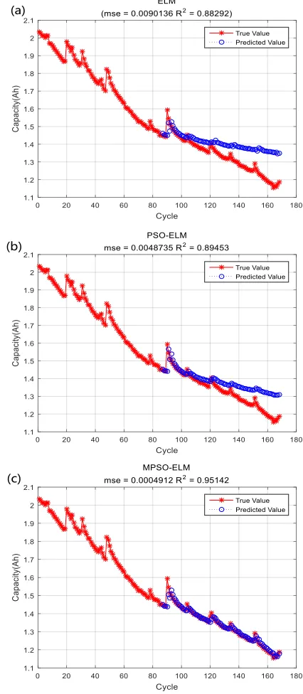
In this paper, the ELM algorithm and the PSO-ELM algorithm are respectively used to compare with the MPSO-ELM algorithm. In Fig.4 (a), Fig.4 (b) and Fig.4 (c), experiments under the same conditions are performed. Fig.4 (a) is the prediction of B5 by the ELM algorithm, Fig.4 (b) is the prediction of B5 by the PSO-ELM algorithm, and Fig.4 (c) is the prediction of the MPSO-ELM method mentioned here. The blue line is the predicted value and the red line is the true value.

Fig.4 (a) is the prediction result of ELM method, there is a big gap between the true value and the predicted value. Fig.4 (b) and Fig.4 (c) are the improved prediction values of ELM method. Compared with Fig.4 (a), its predicted value and true value are basically same. This shows that the ELM algorithm with optimized weights and bias has more accurate prediction result. The error evaluation criteria values of the three methods for B5 are given in Table 2.

(a)

(b)

(c)

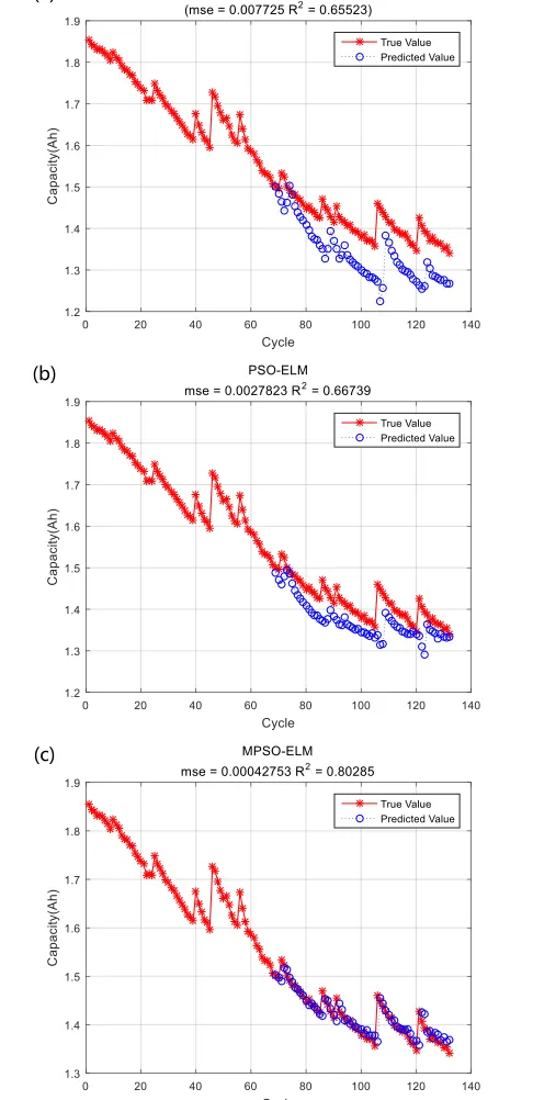
The results predicted by MPSO-ELM algorithm for B6 and B18 are shown in Fig. 5 and Fig. 6, respectively. Similarly, the red line in the figure is the true value of the capacity and the blue line is the predicted value.

In the figure above, Fig.5 (a) is the predicted result of the ELM method, Fig.5 (b) is the predicted result of the PSO-ELM method, and Fig.5 (c) is about the MPSO-ELM method. It is clear from the figure that the predicted value of Fig.5 (c) is closer to the actual value. The values of the three error evaluation criteria for B6 are listed in Table 2.

B18 is also used in three prediction method. Fig.6 is about the prediction results. (a)

(b)

(c)

As can be seen from Fig.6, as the algorithm continues to improve(from Fig.6(a) to Fig.6(c)), the predicted value represented by blue line is getting closer and closer to the true value represented by the red line, that is, the prediction accuracy of the RUL of the lithium battery is getting higher and higher. The prediction results of MPSO-ELM algorithm are closer to the real value than that of the other two algorithms. The values of the three error evaluation criteria for B18 are also listed in Table 2.

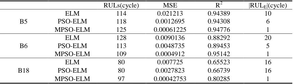
Table 2. Error evaluation criteria for B5, B6 and B18

RULs(cycle) MSE R2 |RULE|(cycle)

B5

ELM PSO-ELM

114 0.021213

0.0012695

0.94389 0.94308

10 6 118

MPSO-ELM 125 0.00061225 0.94776 1

B6

ELM 128 0.0090136 0.88292 20

PSO-ELM 113 0.0048735 0.89453 5

MPSO-ELM 109 0.0004912 0.95142 1

B18

ELM 80 0.007725 0.65523 16

PSO-ELM 80 0.0027823 0.66739 16

MPSO-ELM 97 0.00042753 0.80285 1

From the value of Table2, we can see that for the MSE value, the method proposed in this paper is 0.1 times of the above other two algorithms, and for R2 value, the MPSO-ELM method is closer to 1. RULE reflects the difference between the true value and the predicted value, and the closer to 0, the

more accurate the RUL prediction for lithium battery is, and the values are 1 for the proposed method. The three error evaluation criteria values of MPSO-ELM are better than that of the other two algorithms, therefore, the MPSO-ELM algorithm proposed in this paper has higher prediction ability.

Fig.7 lists 3 different groups of experimental data and the size of the MSE value under the prediction of different algorithms. The smaller the value of MSE, the more accurate the corresponding method is. Different colors represent different algorithms. Among them, the value of the yellow columnar strip is the smallest, that is, the accuracy of the MPSO-ELM algorithm is the highest.

0 0.005 0.01 0.015 0.02 0.025

B5 B6 B18

ELM PSO-ELM MPSO-ELM

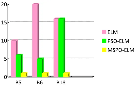
Fig.8 is about the absolute values of RULE for the three algorithms, which are distinguished by

3 different colors. The smaller the RULE value is, the more accurate the forecast result is. The yellow

histogram is much shorter than the red and green. Therefore, it represents the MPSO-ELM algorithm has a higher prediction accuracy.

0 5 10 15 20

B5 B6 B18

ELM PSO-ELM MSPO-ELM

Figure8. The absolute value of RULE for three different algorithms

To further verify the effectiveness of the MPSO-ELM method, we compare the proposed method with some of algorithms in the INTRODUCTION section. In that section, we introduced some related and relevant literatures. [25-29] are based on the ELM algorithm for lithium battery prediction. [25] Using the ELM algorithm to predict the SOC and SOH values of lithium batteries, the RMSE values were 3.1% and 2.4%, respectively. [26] predicts the SOC value of the mobile phone battery with a RMSE of 0.0344. [29] uses the OS-ELM algorithm to estimate the SOC value of a lithium-ion battery, where the MSE value is 0.000065244. The value of R2 is 0.955. However, these articles are based on different datasets. Therefore, the results are not comparable to this article. Both [27] and [28] are experiments on the battery group B5 based on the ELM algorithm, which have been listed in Table 3.

Table 3. Comparison of different methods

Data Algorithm Threshold(Ah) RULs(cycle) |RULE|(cycle)

B5 DE-RVM[7] PF[9] KPF[9] AFSA-PF[9] MSVM[16] PSO-MSVM[16]

The algorithm in [9] is a model-based approach, and the experiment is implemented under three different algorithms. The three algorithms are PF algorithm, KPF algorithm and AFSA-PF algorithm. The improved SVM algorithm proposed in [7] and [16] belongs to the data-driven method. In [7], the differential evolution (DE) algorithm is used to improve the SVM algorithm and the improved DE-SVM algorithm is used to estimate the RUL of the battery B5. [16] compares the PSO-MDE-SVM algorithm with the Multiclass SVM (MSVM) algorithm.

In Table 3, all the algorithms use the same data set, so the experimental results are comparable. We compare the |RULE| values, which reflect the difference between the actual RUL value and the predicted value. The smaller the value, the more accurate the method. Therefore, we can see that the MPSO-ELM algorithm proposed in this paper can more accurately predict the RUL value of lithium batteries. Due to the different thresholds, the |RULE| value is not the same although it has the same

RULs value.

In this part, MSPO-ELM algorithm is first compared with some similar algorithms: ELM and PSO-ELM. Table 2 lists the results. Then the MPSO-ELM algorithm is compared with several algorithms mentioned in the INTRODUCTION section, and the comparison results are given in Table 3. According to the value of the error evaluation standard in the two tables, the algorithm proposed in this paper has a better prediction ability.

5. CONCLUSION

Aiming at the problem that the input weights and bias of ELM are randomly generated, which will affect the prediction results, this paper optimizes the weights and bias. The proposed optimization algorithm is based on the idea of mutation of GA and adds the mutation factor to the particle swarm optimization algorithm so as to improve the ELM algorithm, that is, the MPSO-ELM algorithm. The algorithm was applied to the RUL prediction of lithium-ion batteries. In experiment, we first compare the proposed method with the similar algorithm: ELM and PSO-ELM methods, and then we compare with some methods mentioned in the INTRODUCTION section. All these methods are based on the same data set. The results show that the MPSO-ELM algorithm is an effective RUL prediction method.

ACKNOWLEDGEMENTS

This work received financial support from the National Natural Science Foundation of China (No.71601022), the Natural Science Foundation of Beijing (4173074), the Key Project B Class of Beijing Natural Science Fund (KZ201710028028). And the work supported by Youth Innovative Research Team of Capital Normal University.

References

1. X. Xu and N. Chen, Reliability Engineering & System Safety, 159 (2017) 47. 2. J.M. Tarascon and M. Armand, Nature, 414 (2001) 359.

3. J. Zhang and J. Lee, Journal of Power Sources, 196 (2011) 6007.

5. Y. He, X.T. Liu and C.B. Zhang, Applied energy, 101 (2013) 808.

6. B. Saha, G. Kai, and J. Christophersen, Transactions of the Institute of Measurement & Control, 31 (2009) 293.

7. C.L. Zhang and Y. He, Computational Intelligence & Neuroscience, 1 (2015) 14.

8. H.S. Ramadan, M. Becherif, and F. Claude, International Journal of Hydrogen Energy, (2017). 9. Y. Tian, C. Lu and Z. Wang, Mathematical Problems in Engineering, 3 (2014) 1.

10.L.F. Wu, X. Fu and Y. Guan, Applied Sciences, 6 (2016) 166.

11.A. Nuhic, T. Terzimehic and T. Soczka-Guth, Journal of Power Sources, 239 (2013) 680. 12.A.A. Hussein, IEEE Transactions on Industry Applications, 51 (2015) 2321.

13.AA. Hussein, Applied Power Electronics Conference and Exposition IEEE, (2017) 3122. 14.W. He, N. Williard and M. Osterman, Journal of Power Sources, 196 (2011) 10314. 15.D. Wang, Q. Miao and M. Pecht, Journal of Power Sources, 239 (2013) 253.

16.D. Gao and M. Huang, Journal of Power Electronics, 5 (2017) 1288. 17.M.A. Patil, P. Tagade and K.S. Hariharan, Applied Energy, 159 (2015) 285. 18.D. Gao and M. Huang, Journal of Power Electronics, 17 (2017) 1288. 19.M.A. Patil, P.Tagade and K.S. Hariharan, Applied Energy, 159 (2015) 285.

20.H. Li, D. Pan and C.L. Chen, IEEE Transactions on Systems Man & Cybernetics Systems, 44 (2014) 851.

21.R. Ahila, V. Sadasivam and K. Manimala, Applied Soft Computing, 32 (2015) 23.

22.P. Shi, C. Bu and Y. Zhao, IEEE International Conference on Information Acquisition, (2005) 5. 23.G.B. Huang, Q.Y. Zhu and C.K. Siew, Neurocomputing, 70 (2006) 489.

24.G.B. Huang, H. Zhou and X. Ding, IEEE Transactions on Systems Man & Cybernetics Part B, 42 (2012) 513.

25.A. Densmore and M. Hanif, PowerAfrica, 2016 IEEE PES IEEE, (2016) 184.

26.Z. Wang Z and D. Yang, International Conference on Power Electronics Systems and Applications, (2016):1.

27.D. Gao, M.H. Huang, M and J. Xie, Sae International Journal of Alternative Powertrains, 6 (2017).

28.Y.Y. Jiang, Z. Liu, H. Luo and H. Wang, Journal of Electronic Measurement and Instrumentation, 30 (2016) 179.

29.Y. Zhu, International Journal of Electrochemical Science, 12 (2017) 6895.

30.N. Liang, G. Huang and P. Saratchandran, IEEE Transactions on Neural Networks, 17 (2006) 1411.

31.C.A.C. Coello, G.T. Pulido and M.S. Lechuga, IEEE Transactions on Evolutionary Computation, 8 (2007) 256.

32.D. Simon, IEEE Transactions on Evolutionary Computation, 12 (2008) 702.

33.Y. Shi and R.C. Eberhart, Proc of IEEE Congress Evolutionary Computation. (1998) 69. 34.Y.D. Valle, G.K. Venayagamoorthy and S. Mohagheghi, IEEE Transactions on Evolutionary

Computation, 12 (2008) 171.

35.Z.H. Zhan, J. Zhang and Y. Li, IEEE Systems Man & Cybernetics Society, 39 (2009) 1362. 36.A. Ratnaweera, S.K. Halgamuge and H.C. Watson, IEEE Press, (2004).

37.D. Liu, Y. Luo, L. Guo and Y. Peng, in Proceedings of the IEEE Conference on Prognostics and Health Management (PHM ’13), (2013) 1.

38.R. Razavi-Far, M. Farajzadeh-Zanjani and S. Chakrabarti, IEEE International Conference on Prognostics and Health Management, (2016) 1.

39.R. Khelif, B. Chebel-Morello and N. Zerhouni, Ifac Papersonline, 48 (2015) 761.