Sweatman, M.B. and Quirke, N. (2004) Simulating fluid-solid equilibrium with the Gibbs
ensemble. Molecular Simulation, 30 (1). pp. 23-28. ISSN 08927022
http://
strathprints
.strath.ac.uk/
13476
/
Strathprints is designed to allow users to access the research output of the University
of Strathclyde. Copyright © and Moral Rights for the papers on this site are retained
by the individual authors and/or other copyright owners. You may not engage in
further distribution of the material for any profitmaking activities or any commercial
gain. You may freely distribute both the url (
http://
strathprints
.strath.ac.uk
) and the
content of this paper for research or study, educational, or not-for-profit purposes
without prior permission or charge. You may freely distribute the url
(
http://
strathprints
.strath.ac.uk
) of the Strathprints website.
Self-referential Monte Carlo method for calculating the free energy of crystalline solids
M. B. Sweatman*
Department of Chemical and Process Engineering, University of Strathclyde, Glasgow, G1 1XJ, United Kingdom
共Received 2 March 2005; published 20 July 2005兲
A self-referential Monte Carlo method is described for calculating the free energy of crystalline solids. All Monte Carlo methods for the free energy of classical crystalline solids calculate the free-energy difference between a state whose free energy can be calculated relatively easily and the state of interest. Previously published methods employ either a simple model crystal, such as the Einstein crystal, or a fluid as the reference state. The self-referential method employs a radically different reference state; it is the crystalline solid of interest but with a different number of unit cells. So it calculates the free-energy difference between two crystals, differing only in their size. The aim of this work is to demonstrate this approach by application to some simple systems, namely, the face centered cubic hard sphere and Lennard-Jones crystals. However, it can potentially be applied to arbitrary crystals in both bulk and confined environments, and ultimately it could also be very efficient.
I. INTRODUCTION
There are many Monte Carlo methods关1–11兴 in the lit-erature for calculating the absolute free energy of classical crystalline solids but none of them are entirely satisfactory. Here, I describe a different approach for such systems, a “self-referential”共SR兲Monte Carlo technique for calculating the free energy of classical crystalline solids, both in the bulk and in confined spaces. The aim of this work is to demon-strate the feasibility of this approach by application to some simple crystalline systems, namely, the face centered cubic crystals of hard sphere and Lennard-Jones particles. Al-though this general approach has been considered before by Barnes and Kofke 关12兴 in the context of a “hard rod on a line” system, and there are also some strong parallels with the work of Mon and colleagues关13,14兴who studied lattice systems, the method provided here is quite different and it can potentially be applied to arbitrary crystals whether in bulk or confined environments. The current implementation of this technique is rather inefficient, but in the summary I outline some ideas that should allow this method to be very efficient.
Phase transitions involving crystalline solids are often strongly first order and associated with significant hysteresis. So knowledge of the free energy of crystalline solids is im-portant, particularly in computer simulations where, because of relatively small system sizes, nucleation events can be rare. At this stage it is also important to note a significant technical difference between simulation studies of crystals in bulk and confined environments. For a bulk system the ex-perimental pressure and temperature can be imposed by simulating in the isothermal-isobaric共NPT兲 ensemble. This means that only free-energy differences between competing phases need be determined as a function of pressure to de-cide the location of an equilibrium transition. However, when simulating a confined system we are usually limited to
small systems that do not include the confined system–bulk system interface. So, in general, we cannot impose or mea-sure the bulk共i.e., experimental兲 pressure corresponding to the confined state. Instead, it is essential that the absolute chemical potential is known, because this quantity is the same in the confined and bulk systems at equilibrium. Un-fortunately, we cannot impose the chemical potential on simulated crystals 共i.e., we cannot simulate crystals in the grand-canonical ensemble兲because of difficulties associated with periodic boundary conditions and particle number fluc-tuations共this is explained in detail later兲. Rather, simulations
shouldbe performed with a fixed number of particles and the absolute chemical potential should be measured. For a pure system the chemical potential is simply the Gibbs free ergy per particle of the confined isothermal-isobaric en-semble. So for simulation studies of confined crystals calcu-lation of the absolute Gibbs free energy is essential if conditions inside the pore are to be related to experimental 共or bulk兲conditions, regardless of whether phase behavior is of interest or not.
reference state is exactly the same state as the final state 共hence the term self-referential, coined by Barnes and Kofke 关12兴兲, except that the reference state has a different number of particles共or crystal unit cells to be precise兲. This choice has several distinct advantages that will potentially allow short paths between these two states to be easily defined. They are as follows: 共1兲 a direct path between initial and final states is traversed avoiding first-order phase transitions 共longer paths designed to avoid these transitions are unnec-essary兲,共2兲 the path needs to traverse only relevant degrees of freedom and need not traverse other degrees of freedom or parameters, i.e., the molecular model 共both molecule-molecule and molecule-molecule-wall interactions兲 is constant along the path, and 共3兲 together with the retiling algorithm 共see later兲 only the absolute minimum number of particles need travel this path, i.e., only one crystal unit cell for a bulk system 共in all other methods all particles in the ensemble travel the path兲. These aspects are discussed in more detail in the comparison section below and in the Summary.
Many alternatives exist for calculating free-energy differ-ences 关2,8,9兴, including thermodynamic integration 共TI兲, free-energy perturbation, and “parameter hopping” 共or mul-ticanonical simulation兲as seen in the umbrella-sampling关2兴, Landau free energy关5兴, and phase-switch关4兴approaches. It is possible to couple numerical integration共quadrature兲with each of these techniques to produce an efficient method for traversing the required free-energy difference. In the imple-mentation described below, parameter hopping is used with-out quadrature to traverse the path, i.e., the entire free-energy difference is traversed without any interpolation by a succes-sion of connected hops, and consequently the SR approach described here is not particularly efficient. Some ideas that could dramatically improve its efficiency are discussed in the Summary.
The remainder of this paper is organized as follows. In the next two sections I discuss some issues relating to the moti-vation for this work. Then I describe the SR method as it is applied to the simple systems considered here. I avoid at-tempting a more general definition of the methodology that could be applied to arbitrary crystals, which would be rather complicated, in favor of clarity, which is more important considering that the aim of this work is to validate a new idea. This developed methodology is applied to calculate the chemical potential of pure fcc hard-sphere and Lennard-Jones bulk crystals. Results are presented at conditions of solid-fluid coexistence and compared with existing reference data. Finally, I discuss potential future work including ideas to improve efficiency.
A. The choice of ensemble
In a conventional simulation of a crystalline solid with periodic boundary conditions the number of lattice sites is fixed. Further, in a grand-canonical-ensemble simulation the volume is fixed, and it follows that for a space-filling crystal the lattice site density must also be fixed. If the lattice site density is fixed then, clearly, there is no way that the simu-lated crystal can attain the correct equilibrium lattice site density unless, somehow, it is initiated in this state. This is
the principal reason why space-filling crystals cannot be simulated in the grand-canonical ensemble. Of course, an-other problem has to do with the probability of acceptance of insertion and deletion moves, but this is only a practical problem that might be tackled with sufficient computing re-sources or clever algorithms. The problem concerning the lattice site density is more fundamental. Note that this is not a finite-size effect, i.e., it is not necessarily resolved by simu-lating a sufficiently large system because no matter how large the system one cannot guarantee that it will be initiated with the correct lattice site density. For two-dimensional 共2D兲 crystals, for example, those that form as an adsorbed layer on a surface, the lattice site density is fixed if the simu-lation box area parallel to the layer is fixed. So equilibrium 2D crystals can only be simulated if the simulation box lengths parallel to the surface are allowed to fluctuate. This holds even if the 2D layer is in contact with a fluid phase.
Of course, simulations of pure 共defect-free兲 crystalline solids can be carried out in theNPTensemble for bulk crys-tals and the isothermal-isotension ensemble 共NT兲 for con-fined systems. For a system concon-fined in an ideal slit pore, for example, interfacial tension is fixed in a direction parallel to the slit. Now the lattice site density is free to fluctuate and attain the true equilibrium state. This approach is fine for bulk crystals where the simulated pressure corresponds to experimental pressure. But crystals confined within pores of fixed width 共slit pores, for example兲 do not experience the bulk pressure directly, unless the confined system–bulk sys-tem interface is simulated. Instead, to establish the experi-mental or bulk conditions corresponding to a confined state one must know the chemical potential, because the chemical potential is constant throughout an equilibrium system re-gardless of inhomogeneity. So we would like to simulate confined crystals in the grand-canonical ensemble where the chemical potential is imposed, yet we cannot. Rather, we should simulate them in anNT ensemble andmeasure the absolute chemical potential 共and hence the Gibbs free en-ergy兲to establish experimental共or bulk兲conditions. Despite this, there are several examples 关16–19兴 in the literature where the grand-canonical ensemble has been used to simu-late space-filling crystalline solids and 2D crystals with fixed box area. All this work should be considered carefully, be-cause in every case these are not equilibrium simulations. Note also the simulations by Dominguez and colleagues关20兴 in which crystalline solid free energies for a slit-pore system are calculated in an ensemble in which the slit-pore area is fixed. We can expect that their free-energy calculations and hence their predicted phase transition points are dependent on their choice of slit-pore area, a fact admitted by them when referring to the strain on their simulated crystals.
The key point of this discussion is to emphasize the im-portance of methods for calculating the chemical potential 共or equivalently the Gibbs free energy兲of confined crystals. This is an important factor in the motivation for this current work.
B. Comparison with other approaches
Given the plethora of alternative methods this justification could become exorbitantly long, so this section will concen-trate on comparing the self-referential approach with some of the more popular and robust methods in the literature, in particular the lattice-coupling-expansion TI method 关2兴, the Landau free-energy approach 关5兴, and the phase-switch method关4兴 共these last two methods were not originally de-signed to calculate absolute free energies, but provided the absolute free energy of the reference fluid phase can also be calculated they can clearly be used for this purpose兲. To com-pare these approaches let us consider a cubic phase of ice confined within a slit pore at fixed conditions of pore width, temperature, and interfacial tension 共or equivalently fixed grand potential per unit area of slit兲. As we are using this system as a hypothetical application there is no need to worry about whether this phase does actually exist.
Let us consider the lattice-coupling-expansion TI method first. With this method the共canonical兲Helmholtz free energy is calculated at fixed slit-pore area. The first step in the TI scheme is to introduce a center-of-mass constraint so that subsequent paths can be traversed. The details of this step are not trivial 关2兴 and, indeed, recent work 关21兴 has corrected previous errors associated with this step. Next, we traverse a path that gradually couples the water molecules to their lat-tice sites with strong harmonic springs. Note that orienta-tional关22兴as well as translational coupling of the water mol-ecules might be useful for this material in order to avoid traversing first-order phase transitions along subsequent paths. If orientational coupling is used then it might be ad-vantageous to gradually turn off any electrostatic dipoles on the water molecular model—this could help with the subse-quent expansion stage. Next, the area of the slit pore can be gradually increased until interactions between water mol-ecules are insignificant. Note that the area of the final ex-panded state will depend on whether the electrostatic dipole interactions have previously been turned off关because perma-nent dipole–permaperma-nent dipole interactions decay more slowly共r−3兲 than induced dipole–induced dipole 共or disper-sion兲 interactions 共r−5兲兴. Next, any orientational coupling will need to be gradually turned off. Finally, the water molecule–pore wall interactions will need to be gradually turned off to arrive at the noninteracting Einstein crystal. Note that a further step involving calculating the free energy of the ideal gas 共with orientational degrees of freedom兲 might be needed. Finally, this entire calculation should be repeated for a range of system sizes to ascertain the signifi-cance of finite-size effects induced by simulating in an en-semble with fixed slit-pore area.
Next, consider the Landau free-energy approach applied in anNT ensemble consisting of fixed interfacial tension, number of water molecules, and temperature, where a path from the cubic crystalline phase to fluid water is to be tra-versed. The free energy of this ensemble is simply the water chemical potential multiplied by the number of water mol-ecules. First, an order parameter that can effectively distin-guish different solid and fluid phases must be formulated. Once this is achieved the simulation proceeds by comparing the statistical likelihood of macrostates constrained to narrow ranges of this order parameter—stepping continuously through the order parameter from the crystal to the fluid共or
vice versa兲 generates the required free-energy difference, avoiding any first-order phase transitions. To be successful the resulting fluid phase must be 共meta兲stable. If no stable liquidlike phase exists at the required conditions then a path in thermodynamic space共temperature and interfacial tension in this case兲 might be traversed to ensure the existence of such a fluid state. So some understanding of the phase be-havior of the fluid state is required in advance. Finally, the free energy of the fluid water is obtained by standard meth-ods. The efficiency of this approach depends on the free-energy barrier between initial and final states. The height of this barrier is not known a priori—it will depend on the order parameter, but it will essentially be proportional to the number of particles in the simulation.
Now let us consider the phase-switch method applied, again, in anNT ensemble. This is essentially a parameter-hopping approach that measures the free-energy difference between two states by sampling both states in the same simu-lation. Specialized Monte Carlo共MC兲moves allow the sys-tem to switch from one state to the other 共by performing a global coordinate transformation兲provided the system is suf-ficiently close to special microstates where this switch has a reasonable probability of being accepted. The system is bi-ased to ensure that it approaches these special microstates with sufficient regularity. This is not actually so different from the Landau method above; in this case the bias directs the fluid subsystem toward special “frozen” or fixed fluid configurations that can then be rearranged 共via the global coordinate transformation兲 to generate the crystal. So the same remarks pertain to this approach as to the Landau ap-proach above, except that a different order parameter is needed.
Finally, consider the SR approach. Once again simulations are performed in the NT ensemble. Two steps are per-formed共and are explained in more detail later兲. The first is a single parameter-hopping step that doubles the number of unit cells in the simulation—this is achieved by replication whereby a double-size system is created consisting of two nearly identical 共to within a tolerance兲 single-size systems. The second step allows the coordinates of the newly created water molecules to relax fully from their initial highly con-strained values.
becomes more complex, for example, crystals of proteins and pharmaceuticals confined in structured pores. Enhance-ment of the SR approach in line with ideas outlined in the Summary could potentially lead to it also being a very effi-cient approach.
II. THEORY
Our aim is to calculate the Gibbs-free-energy difference between two crystalline solid systems with differing numbers of unit cells共but are otherwise identical兲. If one system has
munit cells and the other has n⬎m, then the free energy of this structure isx⌬G/共n−m兲 wherexis the number of unit cells and ⌬G is the Gibbs-free-energy difference between these two systems. For a pure crystal the chemical potential is then⌬G/Nc共n−m兲whereNcis the number of particles per
unit cell. So, to be clear, the SR approach is simultaneously both a free-energy difference and an absolute method. It cal-culates the Gibbs-free-energy difference between two sys-tems that differ only in their size, yet because the Gibbs free energy scales linearly with size the absolute Gibbs free en-ergy共and chemical potential for a pure system兲 is obtained automatically. This idea was first expounded by Barnes and Kofke in a slightly restricted sense, i.e., they formulated and applied this SR idea in the canonical ensemble where it is exact only in the thermodynamic limit共although their model system of hard rods was found to be sufficiently large that finite-size effects were unimportant兲. Note also the parallels with the work of Mon. In this work the free-energy differ-ence between lattice systems 共once again in the canonical ensemble兲that differ only in their size is calculated, but lin-earity of the free energy with system size is explicitly not assumed. So this is not a SR approach in the fullest sense defined here.
For a mixture we must also know the difference in chemi-cal potential between each species to obtain the absolute chemical potentials. But this is not the focus of this work, and is a problem with all methods that calculate Gibbs free energies. For alloys, it might be resolved using a semi-grand-ensemble simulation关2兴.
The systems analyzed here are pure bulk crystalline solids with cubic unit cells where each particle only has transla-tional degrees of freedom共denoted byr兲and the discussion below reflects this. Modifications that arise when considering more complex systems, such as confined or molecular crys-tals, will be discussed briefly in the Summary. In this imple-mentation of the SR approach we choose for convenience
n= 2mand⌬Gis split into two contributions. The first mea-sures the free-energy difference between the small 共 single-sized兲 system at pressure Ps and temperature Ts, and the
large共double-sized兲system atPd1andTd1, where one-half of
the double-size system is a replica, to within a tolerance, of the other half. The second contribution measures the free-energy difference between this constrained double-size sys-tem and the unconstrained double-size syssys-tem atPsandTs.
MC schemes to measure each of these contributions are de-scribed below separately. Alternative schemes with different choices forn are possible and discussed in the Summary.
Each scheme is based on parameter hopping, i.e. two neighboring states, labeled a andb, are simulated
simulta-neously in a multicanonical ensemble. The free-energy dif-ference between these two states,⌬Gab, is simply
⌬Gab= −kBTln共pb/pa兲 共1兲
wherepa= 1 −pbis the unbiased probability that the
simula-tion is in macrostatea. This free-energy difference is also the bias needed in a non-Boltzmann sampling regime to ensure
pa=pb.
The Gibbs free energy is related to the corresponding par-tition function⌿ via the fundamental relation
G= −kBTln共⌿兲. 共2兲
Following the arguments put forward by Wilding 关23兴 the isothermal-isobaric partition function for a classical crystal-line solid is presented as
⌿共N,P,T兲=
冕
0 ⬁
dV e−PV⌳
−N
N
冕
V⬘drNe−H共rN兲 共3兲 where H is the configurational contribution to the Hamil-tonian,= 1 /kBTis the inverse temperature,Vis the volume,
and⌳is obtained by integrating momentum degrees of free-dom. The factor N−1 deserves some explanation. Normally this factor, which accounts for double-counting states that have identical quantum wave functions, would beN!. But in Eq.共3兲the particles are not allowed to permute their lattice positions共signaled by the constraint V
⬘
兲. So the number of identical states, allowing for periodic boundary conditions, in now onlyN. Of course, this is not a true partition function because it is not dimensionless. Work by Koper and Reiss suggests that the proper partition function for the NPT en-semble is⌿共N,P,T兲=
冕
0 ⬁
dVP*共V兲e−PV⌳ −N
N
冕
V⬘drNe−H共rN兲
=
冕
0 ⬁
dVP*共V兲e−PVQN 共4兲
where
P*=ln共QN兲
V 共5兲
is the volume-dependent internal pressure, which is distinct from the pressure P imposed by the external reservoir. The deviation of P* from P increases as V decreases, and is thought to be significant only for small systems. In this work this factor is omitted, potentially leading to another source of finite-size error in addition to that induced by periodic boundaries.
The partition function can be reexpressed 关23兴 in a slightly simpler form by “clamping” the position of particle 1,
⌿共N,P,T兲=
冕
0 ⬁
dV e−PVV N
冕
V⬘configu-rational contributions only. This is the final form of the par-tition function used in this work.
A. Doubling and halving
MC moves attempt to double the system 共if it is single sized兲 or halve the system 共if it is double sized兲. These at-tempts are chosen with equal probability. A doubling move doubles the volume and number of particles. Particles are created with coordinates determined by their labels, i.e.,
rj=rj−N+Lx+⌬rj 共7兲
for j=N+ 1 , . . . , 2N, where Lx is a vector, with length Lx,
equivalent to one of the primary single-size simulation box lengths.⌬rjis a random displacement, chosen with uniform
probability from within a sphere of radius␣1Lx, where ␣1
Ⰶ1 is the initial tolerance. A halving move halves the vol-ume and deletes particlesN+ 1 , . . . , 2N.
In addition to these moves, other MC moves ensure tem-perature and pressure equilibration. For temtem-perature equili-bration the position coordinate displacement moves are spe-cialized to improve sampling in the double-size system. In this case two particles, with labels j and j+N, are both moved simultaneously共j is chosen at random兲 by the same amount␦rj, which is chosen as per the usual displacement
selection criteria for particles in the small system. Then one of the particles共jorj+N, chosen randomly with equal prob-ability兲is displaced by a further smaller amount ␦r
⬘
. If the particles exceed their tolerance then the move is rejected, i.e., if兩rj−共rj+N−Lx兲兩⬎␣iLx 共8兲
forj= 1 , . . . ,N共and wherei= 1 in this case兲. If this multiple-move approach were not adopted then only individual multiple-moves within the tolerance criteria would be allowed, and such moves would be very small and inefficient when␣iis small.
Of course, the usual individual particle displacement moves are performed instead in the single-size system, and the po-sition of particle 1 is never moved because it is clamped. To equilibrate pressure the usual volume scaling moves are at-tempted, i.e., the position coordinates of each molecule共 in-cluding the clamped molecule兲 are scaled by randomly choosing a step in the volume with uniform probability on the range ±LV.
The acceptance criteria for these moves are defined to achieve microscopic reversibility. This requires satisfaction of
opon ch
pon acc
=npno ch
pno
acc 共
9兲
wherexis the probability density that the system resides in
an infinitesimal element of coordinates corresponding to mi-crostatex,pon
ch
is the probability of choosing the trial move such that microstateo 共the old state兲 is transformed to mi-crostate n 共the new state兲 given that the system resides in microstateo, andpon
acc
is the probability of accepting this trial move. The acceptance probabilities are related by
pon acc
= min共1,qon acc兲
,
qon acc
=共qno
acc兲−1. 共10兲
From the partition function共6兲we have
⬀V Ne
−PV
e−HdV drN−1 共11兲
and so givenponch andpnoch the ponaccare uniquely defined. Consider molecular coordinate moves first. For the single-size systemqon
acc
is exactly the same as for any conventional isothermal simulation ifpon
ch
=pno ch
. For the double-size system we have
qon acc
= exp关−di共Hn−Ho兲兴 共12兲
as well, where the subscript didenotes the double-size sys-tem corresponding to tolerance ␣i. But now, depending on
the replication tolerance, the value of the configurational en-ergy of the double-size system is approximately double its value for one-half of this system. So fori= 1 we can write
qon acc⬇
exp关− 2d1共Hn h
−Ho
h兲兴 共
13兲
where the superscripthdenotes the Hamiltonian of one-half of the double-size system. This indicates that the constrained double-size system will behave like an unconstrained system at a lower temperature. So, if we setTd1=Ts, where subscript
sdenotes the single-size system, then in general the crystal will contract. This needs to be avoided so that system dou-bling and halving moves are performed efficiently 共see be-low兲. Hence, we instead choose Td1⬎Ts to ensure that the
double-size system does not significantly contract and so that the energy of the constrained double-size system with toler-ance␣1is sufficiently close to twice the energy of the single-size system.
Now consider volume moves where pon ch
=pno ch
. Because particle 1 is clamped we have
qon acc
=n o
=
␥Voe−Hne−P␥Vo
N dV共␥dr兲
N−1
Voe−Hoe−PVo
N dV dr
N−1
=␥Ne−共Hn−Ho兲e−PVo共␥−1兲 共14兲
where␥=Vn/Vo, i.e., precisely the same acceptance criteria
as for conventional isothermal isobaric simulations关2兴. Note that because the tolerance is defined to scale with system size these volume-scaling moves can never violate the tolerance constraints共8兲. However, there is an additional complication for the double-size system. If we consider a crystal of hard spheres and denote the probability that no particle overlaps are generated on attempted compression for the uncon-strained double-size system by pc, then for the constrained
double-size system this probability is roughly
冑
pc, dependingon the replication tolerance. Expansion moves are not af-fected in this way. So in general the constrained double-size system behaves like an unconstrained system at a higher pressure thanPd1. So, just as for particle displacement moves
above, if we setPd1=Psthen in general the crystal will
con-tract. Hence, we instead choose Pd1⬍Ps to ensure that the
volume of the constrained double-size system with tolerance ␣1is sufficiently close to twice the volume of the single-size
Finally, consider doubling and halving moves. These are compound moves that involve a change in volume and a change in particle number. Consider the volume-change sub-move first. This sub-move is most easily defined as the limit of a more general kind of move. That is, consider the move con-sisting of expanding共or shrinking兲an end slab of the simu-lation so that total volume is doubled 共or halved兲. In this case, the end slab of length Lx
⬘
of the simulation box isex-panded 共or contracted兲 by a factor =Lx/Lx
⬘
. By taking thelimitLx
⬘
→0 it is possible to ensure that there are never anyparticles within this end slab. In the case of a doubling move the next submove consists of replicating the particles in the original volume according to the coordinate choices given in Eq.共7兲. In the case of a halving move this submove consists of deleting particlesN+ 1 , . . . , 2N. To ensure that the correct permutation of particle labels is preserved when performing these addition and deletion submoves we must be careful with calculating periodic images. First, before these sub-moves are performed, periodic images should be “unwound” so that particles that have swapped sides are moved back to their nonperiodic positions outside of the original simulation cell. Then the addition or deletion submoves are performed in accordance with Eq. 共7兲. Finally, periodic images are re-applied in accordance with the new simulation cell bound-aries. Note that this convention must also be followed when analyzing the positions of particles j and j+N according to Eq.共8兲.
From Eqs.共6兲and共9兲we have for doubling moves
qsd acc
=
2Vse−d1Hde−2d1Pd1Vs
2Ns
2dVsdr2Ns−1
Vse−sHse−sPsVs
Ns
dVsdrNs−1
冉
dr
Vr
冊
Ns= 2Vr Ns
e−共d1Hd−sHs兲e−Vs共2d1Pd1−sPs兲 共15兲
whereVr= 4共␣iLx兲3/ 3. Becauseqds acc
is defined via Eq.共10兲 we find generally, depending on the replication tolerance, that one of the acceptance probabilities for these doubling and halving moves is very close to 1 while the other is very close to 0. So to improve statistics the double-size system is biased by an amount
exp共s0Ns兲
共Vˆr兲Ns
共16兲
whereVˆr= 4共␣iLˆx兲3/ 3 andLˆxis a fixed and typical value of
Lx. This yields
ln共qsd acc兲
=Ns关s0+ ln共Vr/Vˆr兲兴−共d1Hd−sHs兲
−Vs共2d1Pd1−sPs兲+ ln共2兲 共17兲
for doubling and halving moves. None of the other types of MC move are affected by this bias. The initial tolerance␣1is chosen to ensure that the acceptance probability of a dou-bling move is not too small 共i.e., Hd⬃2Hs兲, while 0 is
chosen to ensure equal sampling of single- and double-size systems.
B. Relaxation
Having transformed the single-size system to a strained double-size system we now need to relax the con-straint, measuring the free-energy difference between the constrained double-size system and the unconstrained double-size system. Potentially the most efficient way of achieving this is with quadrature, i.e., calculating the rate of change of free energy at many points distributed along the required path and then integrating along the path on the basis of an interpolation scheme. But in this work, which is fo-cused on the feasibility of the SR approach, simple param-eter hopping is employed instead, which calculates the free-energy difference between the two end points of a hop, and then connects very many hops together to traverse the re-quired path.
For each hop a multicanonical simulation is performed that samples states consistent with␣iand␣i+1, i.e., each hop
consists of a “dual-canonical” simulation. Relaxing and con-straining moves are allowed that enable a system with Nd
particles at pressure Pi, temperatureTi, and tolerance ␣i to
switch back and forth to a system at pressurePi+1,
tempera-ture Ti+1, and tolerance ␣i+1 共note that the particles
them-selves are not moved during these switches兲. Relaxing moves are attempted if the double-size system is constrained while constraining moves are attempted共with equal probability兲if the double-size system is relaxed. A path is traced thorough 共P,T,␣兲 space such that the initial point 共Pd1,Td1,␣1兲 is
connected to the final point共Ps,Ts,␣m兲viam− 2 other points
共corresponding tom− 1 separate multicanonical simulations兲 where the final tolerance is sufficiently large that it no longer has any significant effect on the system, i.e., the free-energy difference between 共Ps,Ts,␣m−1兲 and 共Ps,Ts,␣m兲 is
negli-gible. The path is easily defined;=␣i+1/␣i can be set to a
constant, while a simple algorithm, described below, sets
⌬P=Pdi+1−Pdiand⌬T=Tdi+1−Tdito ensure that the average
particle and energy densities of each system do not stray too far from those of the unconstrained system atPsandTs. In
addition to these relaxing and constraining moves the same particle displacement and volume change moves as described above are also allowed.
The acceptance ratio for relaxing moves ifpich共i+1兲=p共chi+1兲iis
qi共i+1兲 acc
=
冉
Vr,iVr,i+1
冊
Nse−Hd共di+1−i兲e−Vd共di+1Pdi+1−iPi兲
=−3Nse−Hd共di+1−i兲e−Vd共di+1Pdi+1−iPi兲. 共18兲
For constraining moves the acceptance ratio is共qiacc共i+1兲兲−1. Finally, to improve statistics we bias the ith state by exp共diNsi兲 so that relaxed and constrained states are
sampled equally. The acceptance ratio for these moves is then
qi共i+1兲 acc
=−3Nse−Hd共di+1−i兲e−Vd共di+1Pdi+1−iPi兲eNs共di+1i+1−dii兲
共19兲
where1= 0.
⌬G=Ns兵0+m−kBTln关Vˆr共␣m兲兴其. 共20兲
There is no unique way of defining an algorithm for cal-culating the pressure and temperature steps ⌬P and⌬T. In this work it is defined for both pressure and temperature as follows. First, target volumes and configurational energies are defined for the double-size system, Vd
t
= 2具V典s and Ed t
= 2具E典s, respectively, where the angular brackets denote an
ensemble average. Then, Pd1 and Td1 are chosen such that
具Vd1典⬵Vd t
and具Ed1典⬵Ed t
and the indices kV and kE are set
equal to 0. The average volume and energy are measured for each ␣i. These indices are set to zero if 具Vdi典⬎Vd
t
or 具Edi典
⬎Ed t
, respectively, while they are increased by 1共to a maxi-mum of 3兲if具Vdi典⬍Vd
t
or具Edi典⬍Ed t
, respectively. For each ␣i+1 the pressure and temperature steps are defined as
⌬P=共Ps−Pdi兲
m−i min
共
kV,m−i兲
,⌬T=共Ts−Tdi兲
m−i min
共
kE,m−i兲
. 共21兲III. RESULTS FOR SIMPLE SYSTEMS
The aim of this work is to test and validate the self-referential method described above. Simple model crystals are ideal for this purpose. Hard sphere and Lennard-Jones 共LJ兲face centered cubic crystals are chosen because of the availability of reference data. The hard sphere and shifted-force LJ potentials are
HS共r兲=
再
⬁, r⬍d, 0, r艌d,
冎
LJ sf共
r兲
=
再
4共x−12−x−6兲−
LJ共rc兲−共r−rc兲LJ
⬘
共rc兲, r⬍rc,0, r艌rc,
冎
共22兲
respectively, wherex=r/,ris the pair separation, the prime indicates the derivative with respect to separation, and LJ
= 4共x−12−x−6兲.
The perfect共defect-free兲fcc hard sphere crystal is simu-lated at fluid-solid coexistence, i.e., at a reduced pressure 关23兴ofPs*=Psd3/kBT= 11.49, whered is the hard sphere
di-ameter共note that in Ref.关23兴the reduced coexistence pres-sure is calculated with an uncertainty of ±0.09兲. Temperature is arbitrary for this system. Simulations with Ns= 108 and
256 are performed to examine finite-size effects, which are expected to vary with system size with a leading-order con-tribution proportional to 1 /Nd. Statistical errors are
calcu-lated in the usual way关24兴using block averages. Regarding the probabilities for choosing each trial move, i.e.,pon
ch
=pno ch
, they are in the ratio 1 :Ns
−1
:Ns −1
for displacement, volume, and doubling and halving moves during the replication stage, and 1 :Nd−1: 1 for displacement, volume, and relaxation or
constraining moves during the relaxation stage.
Simulation parameters and results are given in Table I. I choosePd*1= 6.375 and ␣1= 0.001/Lˆx. The final result is*
=/kBT= 16.08± 0.02. These results confirm共within
statisti-cal error兲 the validity of the result in Ref. 关23兴 for hard sphere fluid–perfect fcc solid coexistence because the共very accurate兲 equation of state of Kolafa et al. 关25兴 for a hard sphere fluid gives*= 15.99± 0.10 atP*= 11.49± 0.09.
For the perfect fcc shifted-force LJ crystal at its triple point, i.e., at a reduced pressure and temperature of P*
=P3/= 0.001 82 and T*=kBT/= 0.56, one simulation
with Ns= 256 is performed. Simulation parameters and
re-sults are given in Table II. I choosePd*1= 0,Td*1= 0.7616, and
␣1= 0.01/Lˆx. The final result is *=/= −3.20± 0.02,
al-TABLE I. Simulation parameters and results for the SR method applied to the fcc hard sphere crystal.Ns
is the number of particles in the single-size simulation and “Trials” is the total number of attempted MC moves—dividing bymgives the number for each relaxation simulation.is the tolerance ratio共see the text兲 in each relaxation simulation and=0+mis the total chemical potential. The numbers in parentheses are statistical errors to one standard deviation.
Type Ns m Trials共106兲 0* m* *
Replication 108 50 1.2311共6兲
Relaxation 108 2500 10 000 1.00268 14.769共14兲 16.000共14兲
Replication 256 100 1.2367共7兲
[image:8.612.109.502.117.199.2]Relaxation 256 5000 40 000 1.00134 14.811共12兲 16.048共12兲
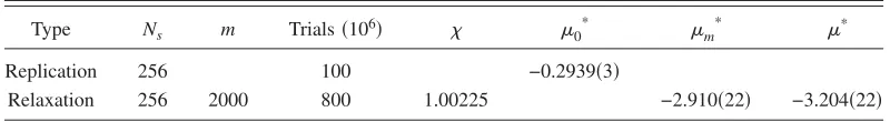
TABLE II. As for Table I except that the shifted-force LJ crystal is simulated.
Type Ns m Trials共106兲 0* m
* *
Replication 256 100 −0.2939共3兲
[image:8.612.106.506.678.733.2]though this does not include an analysis of finite-size effects because of the numerical expense involved. These results agree well with those of Errington and co-workers关26兴and Sweatman and Quirke 关27兴, which together give * = −3.23± 0.02共the gas phase result from a gas-liquid Gibbs simulation关27兴兲.
IV. SUMMARY
The SR methodology described above is appropriate for simple atomic systems that form bulk crystalline solids with cubic unit cells. But this method is potentially very general, and is easily generalized to treat molecular crystals formed from noncubic unit cells. When treating molecular crystals it will be important to constrain internal molecular degrees of freedom in an appropriate manner during replication. For frozen internal molecular degrees of freedom 共such as the orientation of water molecules in ice兲a constraint is needed in much the same way as it is needed for molecular position coordinates. These types of constraint will increase the path length substantially. For nonfrozen molecular degrees of freedom 共such as the orientation of nitrogen in its orienta-tionally disordered crystalline  phase 关28兴兲 the constraint can be much weaker and should not contribute significantly to the numerical effort required to traverse the path. Con-strained molecular degrees of freedom need to be treated in the same way as position coordinates, i.e., constrained on system doubling and then gradually relaxed. The same meth-odology can be employed to treat confined crystals with at least one degree of translational invariance, such as crystals confined in rigid slit pores. In this case pressure should be replaced by grand-potential density 共or interfacial tension兲 and simulations are performed in theNT ensemble by al-lowing fluctuations in simulation box vertices parallel to the translational invariance. Further work is required to investi-gate the possibility of including defects in the free-energy calculation.
The approach described above is not yet efficient. The overwhelming amount of CPU time is spent performing the relaxation stage. For example, for the double-size Lennard-Jones system the 5000 connected hops that traverse the re-laxation path required about six days of computation on a standard desktop 共3.0 GHz兲 PC. There are two reasons for this. First, the free-energy difference between the single- and double-sized systems is large, resulting in a long path length. Second, the parameter hopping approach, although robust, is not efficient. Future work will aim to improve this aspect and
make comparison with other methods. The most obvious idea for improving efficiency is to implement thermody-namic integration共perhaps along the lines described in Ref. 关14兴兲, rather than parameter hopping, as the technique used to relax the double-size system from its initially highly con-strained state to its fully relaxed state. This could potentially reduce the number of individual relaxation simulations from several thousand to less than 100, consequently improving efficiency by perhaps 1 to 2 orders of magnitude. Another possibility is to attempt to adapt Tilwani and Wu’s ingenious retiling algorithm 关29兴, which has been developed for 2D disk systems, to general 3D crystalline solids. This would then allow the large system to be only slightly larger than the small system, say one unit cell larger for a bulk crystal rather than double size, resulting in a much shorter path between initial and final states. Combination of both these efficiency enhancements could perhaps yield a methodology several or-ders of magnitude faster than the current implementation for typical simulations.
The SR approach developed above can be considered a reinvention of the SR approach described by Barnes and Kofke 关12兴, although there are some significant differences. In their work they considered for convenience a system of 1D hard rods on a line, which they argue can be considered a primitive form of crystal in a limited sense. They cast their canonical partition function in terms of vibrational modes, and use free-energy perturbation to traverse the path between single-size and double-size systems. In contrast, this work employs parameter hopping to traverse between the two subsystems—a technique that they also suggest as being worthy of investigation as it has the advantage of being re-versible 共see their work for a discussion of this兲. They also work in the canonical ensemble rather than the isothermal-isobaric ensemble used here, potentially leading to additional ensemble-induced finite-size effects 共although their system was sufficiently large that these effects were not significant兲. They conclude with some suggestions for further work con-cerning the inclusion of temperature and higher dimensions so that more realistic 2D and 3D crystals can be treated. These concerns are effectively answered here. However, this work demonstrates that both the temperature and pressure need to be manipulated during the SR process to ensure that it is feasible.
ACKNOWLEDGMENTS
I sincerely thank Nick Quirke for advice with this work and his tireless support and encouragement over the years.
关1兴J. F. Lutsko, D. Wolf, and S. Yip, J. Chem. Phys. 88, 6525
共1988兲.
关2兴B. Smit and D. Frenkel,Understanding Molecular Simulation: From Algorithms to Applications 共Academic, New York, 1996兲.
关3兴D. Frenkel and A. J. C. Ladd, J. Chem. Phys. 81, 3188共1984兲.
关4兴A. D. Bruce, N. B. Wilding, and G. J. Ackland, Phys. Rev.
Lett. 79, 3002共1997兲.
关5兴R. M. Lynden-Bell, J. S. van Duijneveldt, and D. Frenkel, Mol. Phys. 80, 801共1993兲.
关6兴G. Grochola, J. Chem. Phys. 120, 2122共2004兲.
关7兴A. P. Lyubartsevet al., J. Chem. Phys. 96, 1776共1992兲.
关8兴P. A. Monson and D. A. Kofke, Adv. Chem. Phys. 115, 113
关9兴J. M. Rickman and R. LeSar, Annu. Rev. Mater. Res. 32, 195
共2002兲.
关10兴S. Y. Sheu, C. Y. Mou, and R. Lovett, Phys. Rev. E51, R3795
共1995兲.
关11兴N. B. Wilding and A. D. Bruce, Phys. Rev. Lett. 85, 5138
共2000兲.
关12兴C. D. Barnes and D. A. Kofke, Phys. Rev. E 65, 036709
共2002兲.
关13兴K. K. Mon, Phys. Rev. Lett. 54, 2671共1985兲.
关14兴K. K. Mon and K. Binder, Phys. Rev. B 42, 675共1990兲.
关15兴P. D. Beale, Phys. Rev. E 66, 036132共2002兲.
关16兴R. Radhakrishnan and K. E. Gubbins, Mol. Phys. 96, 1249
共1999兲.
关17兴R. Radhakrishnan, K. E. Gubbins, and M. Sliwinska-Bartkowiak, J. Chem. Phys. 116, 1147共2002兲.
关18兴K. G. Ayappa and C. Ghatak, J. Chem. Phys. 117, 5373
共2002兲.
关19兴M. Miyahara and K. E. Gubbins, J. Chem. Phys. 106, 2865
共1997兲.
关20兴H. Dominguez, M. P. Allen, and R. Evans, Mol. Phys. 96, 209
共1999兲.
关21兴J. M. Polsonet al., J. Chem. Phys. 112, 5339共2000兲.
关22兴L. A. Baez and P. Clancy, Mol. Phys. 86, 385共1995兲.
关23兴N. B. Wilding, Comput. Phys. Commun. 146, 99共2002兲.
关24兴M. P. Allen and D. J. Tildesley,Computer Simulation of Liq-uids共Clarendon Press, Oxford, 1987兲.
关25兴J. Kolafa, S. Labik, and A. Malijevsky, Phys. Chem. Chem. Phys. 6, 2335共2004兲.
关26兴J. R. Errington, P. G. Debenedetti, and S. Torquato, J. Chem. Phys. 118, 2256共2003兲.
关27兴M. B. Sweatman and N. Quirke, Mol. Simul. 30, 23共2004兲.
关28兴E. J. Meijeret al., J. Chem. Phys. 92, 7570共1990兲.