Optimized Energy Aware 5G Network Function Virtualization

Optimized Energy Aware 5G Network

Function Virtualization

AHMED N. AL-QUZWEENI , AHMED Q. LAWEY, TAISIR E. H. ELGORASHI, AND JAAFAR M. H. ELMIRGHANI, (Senior Member, IEEE)

School of Electronic and Electrical Engineering, University of Leeds, Leeds LS2 9JT, U.K.

Corresponding author: Ahmed N. Al-Quzweeni ([email protected])

This work was supported in part by the Engineering and Physical Sciences Research Council (ESPRC), in part by the INTERNET under Grant EP/H040536/1, and in part by the STAR Projects under Grant EP/K016873/1.

ABSTRACT In this paper, network function virtualization (NFV) is identified as a promising key technology, which can contribute to energy-efficiency improvement in 5G networks. An optical network supported architecture is proposed and investigated in this paper to provide the wired infrastructure needed in 5G networks and to support NFV toward an energy efficient 5G network. In this paper, the mobile core network functions, as well as baseband function, are virtualized and provided as VMs. The impact of the total number of active users in the network, backhaul/fronthaul configurations, and VM inter-traffic are investigated. A mixed integer linear programming (MILP) optimization model is developed with the objective of minimizing the total power consumption by optimizing the VMs location and VMs servers’ utilization. The MILP model results show that virtualization can result in up to 38% (average 34%) energy saving. The results also reveal how the total number of active users affects the baseband virtual machines (BBUVMs) optimal distribution whilst the core network virtual machines (CNVMs) distribution is affected mainly by the inter-traffic between the VMs. For real-time implementation, two heuristics are developed, an energy efficient NFV without CNVMs inter-traffic (EENFVnoITr) heuristic and an energy efficient NFV with CNVMs inter-traffic (EENFVwithITr) heuristic, both produce comparable results to the optimal MILP results. Finally, a genetic algorithm is developed for further verification of the results.

INDEX TERMS 5G networks, backhaul, BBU, energy efficiency, fronthaul, genetic algorithm, IP over WDM, network function virtualization, NFV.

I. INTRODUCTION

According to Cisco Visual Networking Index, mobile data traffic will witness seven pleats between 2016 and 2021 and will grow at a Compound Annual Growth Rate (CAGR) of 46% reaching 48.3 exabytes per month by 2021 [2]. This growth is driven by a number of factors such as the enormous amount of connected devices and the development of data-greedy applications [3]. With such a tremendous amount of data traffic, a revolutionary mobile network architecture is needed. Such a network (5G) will contain a mix of a multiple access technologies supported by a significant amount of new spectrum to provide different services to a massive number of different types of users (eg., IoT, personal, industrial) at high data rate, any time with potentially less than 1 ms latency [4]. 5G networks are expected to be operational by

The associate editor coordinating the review of this manuscript and approving it for publication was Irfan Ahmed.

2020 where a huge number of devices and application will use it [5]. Users, applications, and devices of different kinds and purposes need to send and access data from distributed and centralized servers and databases using public and/or private networks and clouds. To support these requirements, 5G mobile networks have to possess intelligence, flexible traffic management, adaptive bandwidth assignment, and at the forefront of these traits is energy efficiency. Informa-tion and CommunicaInforma-tion Technology (ICT) including ser-vices and deser-vices are responsible for about 8% of the total world energy consumption [6] and contributed about 2% of the global carbon emissions [7]. It is estimated that, if the current trends continue, the ICT energy consumption will reach about 14% of the total worldwide consumption by 2020 [6].

There have also been various efforts from researchers on reducing the power consumption and improving the energy-efficiency in mobile networks [8] and 5G networks. For

instance, the authors in [9] focused on the power consumption of base stations. They proposed a time-triggered sleep mode for future base stations in order to reduce the power consump-tion. The authors in [10] investigated the base stations compu-tation power and compared it to the transmission power. They concluded that the base station computation power will play an important role in 5G energy-efficiency. The authors of [11] developed an analytical model to address the planning and the dimensioning of 5G Cloud RAN (C-RAN) and compared it to the traditional RAN. They showed that C-RAN can improve the 5G energy-efficiency. The research carried out in [12] focused on offloading the network traffic to the mobile edge to improve the energy-efficiency of 5G mobile networks. The authors developed an offloading mechanism for mobile edge computing in 5G where both file transmission and task computation were considered.

Virtualization has been proposed as an enabler for the optimum use of network resources, scalability, and agility. In [13] the authors stated that NFV is the most impor-tant recent advance in mobile networks where among its key benefits is the agile provisioning of mobile functions on demand. The fact that it is now possible to separate the functions form their underlying hardware and transfer them into software-based mobile functions as well as pro-vide them on demand, presents opportunities for optimizing the physical resources and improving the network energy efficiency.

In this paper, network function virtualization is identified as a promising key technology that can contribute to the energy-efficiency improvement in 5G networks. In addition, an optical network architecture is proposed and investigated in this paper to provide the wired infrastructural needed in 5G networks, and to support NFV and content caching. In the literature, NFV was investigated either in mobile core net-works [14]–[16] or in the radio access network [17]–[19] of the mobile network and mostly using pooling of resources such as the work in [20], [21]. In contrast, virtualization in this paper is not limited to a certain part in the mobile network, but is applied in both the mobile core network and the radio access network. Moreover, it is not confined to pooling the network resources, but is concerned with mobile functions-hardware decoupling and considers con-verting these functions into software-based functions that can be placed optimally. For instance, instead of having a dedi-cated hardware in RAN to implement baseband processing for each remote radio head and another for user policy in the core network, two virtual machines can share a single general purpose node to implement these functions. In such way the amount of hardware could be reduced to save energy. In addition, packing and hosting VMs close to the user results in short traffic path which results in low traffic induced power.

A Mixed Integer Linear Programming model, real-time heuristics and Genetic Algorithm are developed in this paper with the goal of improving the energy-efficiency in 5G mobile networks.

FIGURE 1. Evolved packet system architecture.

II. NFV IN 5G NETWORKS

According to the third generation partnership project (3GPP) the evolved packed core (EPC) is an important step change [22]. There are four main functions in the EPC [23], [24] illustrated in Fig. 1: the packet data network gateway (PGW), the serving gateway (SGW), the mobility and management entity (MME), and the policy control and charging role function (PCRF).

FIGURE 2. The proposed architecture for Energy Efficient NFV in 5G.

FIGURE 3. The candidate locations for hosting VM in the proposed architecture.

The hosting nodes (ONU, OLT and IP over WDM nodes) might host one VM or more than one VM of the same or different types, bringing forth the creation of small clouds, or ‘‘Cloudlets’’. Therefore, the proposed architecture will provide an agile allotment of services and processes through flexible distribution of VMs over the optical network (PON and IP over WDM network), which is one of the main con-cerns of this work in minimizing the total power consump-tion. Based on this architecture, a MILP formulation has

been developed with the overall aim of minimizing power consumption.

III. FRONTHAUL AND BACKHAUL CONFIGURATION AND THE AMOUNT OF BASEBAND PROCESSING WORKLOAD

This section illustrates the configuration of the fronthaul and backhaul used in the proposed network; so that the ratio of the backhaul to the fronthaul data rate could be calculated. Fronthaul is the network segment that connects the remote radio head (RRH) to the baseband unit (BBU) [30], whilst the network segment that connects the BBU to the mobile core network (CN) is called ‘‘backhaul’’ [31]. The internal inter-face of the fronthaul is defined as a result of the digitization of the radio signal according to a number of specifications. The well-known and most used specification among radio access network (RAN) vendors is the Common Public Radio Inter-face (CPRI) specification [32] which is implemented using digital radio over fiber (D-RoF) techniques. On the other hand, the backhaul interface leverages Ethernet networks as they are the most cost effective network for transporting the backhaul IP packets [33], [34].

In order to adequately determine the data rate in each network segment (backhaul and fronthaul), we will start with the physical layer of the current mobile network which is the Long-Term Evolution (LTE) network. The LTE network uses single-carrier frequency-division multiple access (SC-FDMA) uplink (UL), whilst orthogonal frequency-division multiple access (OFDM) is used in the downlink (DL) [35]. In both techniques, the transmitted data are turbo coded and modulated using one of the following modulation formats: QPSK, 16QAM, or 64QAM with 15 kHz subcarriers spac-ing [36]. A generic frame is defined in LTE which has 10 ms duration and 10 equal-sized subframes. Each subframe is divided into two slot periods of 0.5 ms duration [37]. Depend-ing on the cyclic prefix (CP) used, slots in OFDMA have either 7 symbols for normal CP or 6 symbols for extended CP [38]. Fig. 4 illustrates an LTE downlink frame with normal CP. In the LTE frames, a resource element (RE) is the smallest modulation structure which has one subcarrier of 15 kHz by one symbol [39]. Resource elements are grouped into a physi-cal resource block (PRB) which has dimensions of 12 consec-utive subcarriers by one slot (6 or 7 symbols). Therefore, one PRB has a bandwidth of 180 kHz (12×15 kHz). Different transmission bandwidths use different number of physical resource blocks (PRBs) per time slot (0.5 ms) which are defined by 3GPP [40]. Fig. 5 illustrates the LTE downlink resource grid. For instance, 10 MHz transmission bandwidth has 50 PRBs whilst 20 MHz has 100 PRBs [41]. If 10 MHz bandwidth is used with 16 QAM (6 bits/symbol) and 7 OFDM symbols (short CP), we have

50RB×12subcarriers

RB ×

7symbols subcarrier ×

6bits(QAM)

symbol

0.5ms times lot

=50.4Mbps (1)

FIGURE 4. LTE downlink frame with normal CP.

FIGURE 5. LTE downlink resources grid.

It is worth mentioning that for each transmission antenna, there is one resource grid (50 PRBs for 10 MHz); there-fore in 2×2 MIMO the previous data rate is doubled (100.8 Mbps) [42].

The transmission of user plane data is achieved in the form of In-phase and quadrature (IQ) components that are sent via one CPRI physical link where each IQ data flow represents the data of one carrier for one antenna that is called Antenna-Carrier (AxC) [43]. Two main parameters affect the data carried by AxC, [42]:

Sampling frequency which is calculated as: subcarrier BW (15 kHz) times the FFT window (size). The FFT size is chosen to be the least multiple of 2 that is greater than the ratio of the radio signal bandwidth to the subcarrier BW. For instance, if the radio bandwidth is 10 MHz, the FFT size is the least multiple of 2 that is greater than 666.67 (10 MHz / 15 kHz) which is 1028 (210). In this case the sampling frequency is calculated as 150 kHz×1024 = 15.36MHz. Using the same approach, the sampling frequency at 20 MHz radio bandwidth system is 30.72 MHz.

IQ sample width (M-bits per sample): According to the CPRI specification, the IQ sample width supported by CPRI is between 4 and 20 bits per sample for I and Q in the uplink and it is between 8 and 20 in the downlink [43]. For instance, with M = 15 bits per sample; one AxC contains 15 bits per sample for I and 15 bits per sample for Q which are 30 (2 ×M) bits per sample I and Q which are transported in

sequence:I0Q0I1Q1. . .I14Q14. The IQ sample data rate can be calculated by multiplying the number of bits per sample by the sampling frequency. For instance; for a radio bandwidth of 10 MHz (fs=15.36 MHz) and IQ samples 15 (M=15) the IQ data rate is:

(2×M)×fs = 30bitssample×15.36MHz

=0.4608Gbps (3)

CPRI data rate is designed based on the Universal Mobile Telecommunications System (UMTS) chip rate [43] which is 3.84 Mbps [44], [45]. Therefore, one basic CPRI frame is created every Tc=260.416 ns (1/3.84 MHz) and this duration should remain constant for all CPRI options and data rates. According to CPRI specification in [43], one basic CPRI frame consists of 16 words indexed (W= 0. . . 15), where the first word is reserved for control. The length of the frame word (T) depends on the CPRI line rate as specified by CPRI specification in [43]. Accordingly, the transmission of AxC data will be expanded by a factor of 16/15 (15 bits payload, 1 bit control and management). In addition to the sampling rate fs that is calculated earlier, AxC data needs to be coded using either 8B/10B or 64B/66B.

To put all these calculations together, let’s start with the number of bits per word in the CPRI frame. The number of bits per word is equal to the total number of bits per frame divided by the frame payload words (15 words). Recall that the frame duration should be constants (206.416 ns); therefore:

(no of bits per word×15words) samples of IQ fIQ

=260.416ns (4)

no of bits per wordNbpw=fIQ×260.416ns

15 . (5) One CPRI frame word hasNbpw bits, since the CPRI frame has 16 words:

NbpF =Nbpw×(15payload words)+Nbpw

×1control word (6)

NbpF =Nbpw×(15+1)= fIQ×260.416ns

15 ×16 (7) To calculate the data rate in one CPRI frame

NbpF 260.416ns =

fIQ×260.416ns

15 ×16

260.416ns =fIQ× 16

15 (8) By replacingfIQwith 2×M ×fswhereM is defined earlier

as the number ofIQbits.

In addition, AxC data are coded by either 8B/10B or 64B/66B. By putting these together, the CPRI data rate is calculated as

2×M×fs×

16

15×Lcoding (9)

Finally, the ratio of the backhaul to fronthaul data rate is calculated as:

backhaul (IP)data rate fronthaul(CPRI)data rate =

44.0496Mbps

327.68Mbps ×100%

FIGURE 6. Candidate locations for hosting VMs in the proposed architecture.

Therefore, depending on coding, sampling, quantization, and other parameters; the baseband processing adds overheads to the backhaul traffic as it passes through the BBU. In this work the ratio (13.44%) calculated in (10) is used in our model, whilst the amount of workload in Giga Operation Per Second (GOPS) needed to process one user traffic is used based on the following relation which is explained in [46]:

wl=

30·A + 10·A2 + 20M 6 ·C·L

· R

50 (11)

where:

wl: is the baseband workload in (GOPS) needed to process one user traffic,

A: number of antennas used, M: modulation bits,

C: the code rate,

L: number of MIMO layers,

R: number of physical resource blocks allocated for the user.

IV. MILP MODEL

This section introduces the MILP model that has been devel-oped to minimize the power consumption due to both pro-cessing by virtual machines (hosting servers) and the traffic flow through the network. As mentioned in the previous section, the MILP model considers an optical-based archi-tecture with two types of VMs (BBUVM and CNVMs) that could be accommodated in ONU, OLT and/or IP over WDM as in Fig. 6. The maximum number of VM-hosting servers considered was 1, 5, and 20 in ONU, OLT, and IP over WDM nodes respectively, which is commensurate with the node size and its potential location and hence space limitations (together with the size of exemplar network considered in the MILP). All VM-hosting servers were considered as sleep-capable servers for the purpose of VM consolidation (bin packing).

For a given request, the MILP model responds by selecting the optimum number of virtual machines and their location so that the total power consumption is minimized.

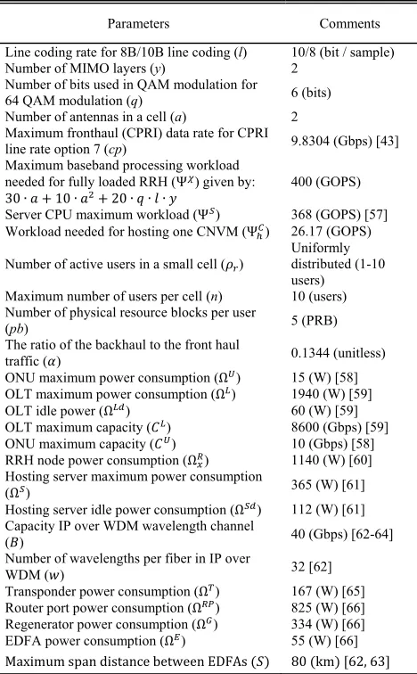
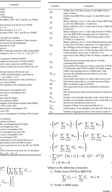
The developed MILP model is defined by a set of indices, parameters and variable which are listed in Table 1, Table 2 and Table 3 respectively.

TABLE 1.Energy efficient NFV MILP model indices.

The total power consumption is composed of:

1) The power consumption of RRHs and ONUs

X

x∈U 

R_x +

U

CU. 

 X

h∈H X

r∈R X

y∈TN x

λR h,r,x,y

+ X

p∈H X

q∈H:p6=q X

y∈TN x ∩H

λT p,q,x,y



 

 (12)

2) The power consumption of the OLTs

X

x∈L 

LdLd+

L_−Ld

CL . 

 X

h∈H X

r∈R X

y∈TN x

λR h,r,x,y

+ X

p∈H X

q∈H:p6=q X

y∈TN x ∩H

λT p,q,x,y



 

 (13)

3) The power consumption of the IP over WDM network

RP_·X m∈N

3m !

+ 

RP· X

m∈N X

n∈NN m

Wm,n 



+ 

T · X

m∈N X

n∈NN m

Wm,n 

+



E· X

m∈N X

n∈NN m

Am,n·fm,n 



+ 

G· X

m∈N X

n∈NN m

N_mG_,n·Wm,n 

 (14)

4) The total power consumption of VMs and hosting servers

X

h∈H

Sd _·9i h+σhχ

+9f

h·

S_−Sd ₍₁₅₎

The model objective is to minimize the total power con-sumption as follows:

MinimizeX

x∈U 

R_x +

U

CU. 

 X

h∈H X

r∈R X

y∈TN x

λR h,r,x,y

+ X

p∈H X

q∈H:p6=q X

y∈TN x ∩H

λT p,q,x,y



 

TABLE 2. Energy-efficient NFV MILP model parameters.

+X

x∈L 

Ld+

L_−Ld

CL . 

 X

h∈H X

r∈R X

y∈TN x

λR h,r,x,y

+ X

p∈H X

q∈H:p6=q X

y∈TN x∩H

λT p,q,x,y



 



TABLE 3.Energy-efficient NFV MILP model variables.

+ RP·X

m∈N

3m !

+ 

RP· X

m∈N X

n∈NN m

Wm,n 



+ 

T · X

m∈N X

n∈NN m

Wm,n 

+



E· X

m∈N X

n∈NN m

Am,n·fm,n 



+ 

G· X

m∈N X

n∈NN m

N_mG_,n·Wm,n 



+X

h∈H

Sd _·9i

h+σ

χ h

+9f

h·

S_−Sd

∀r∈R,∀h∈H (16)

Subject to the following constraints: 1) Traffic from CNVM to BBUVM

X

p∈H

λB p,h=α·

X

r∈R

λR

h,r ∀h∈H (17)

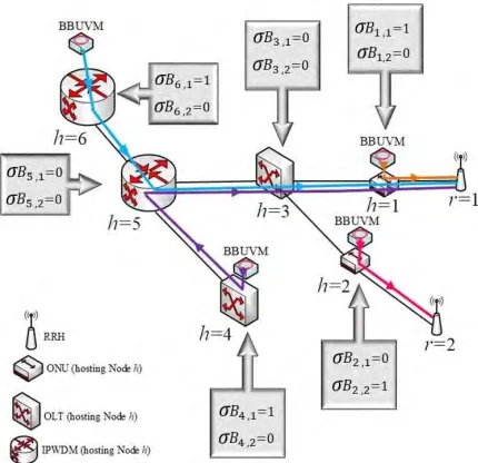
FIGURE 7. BBUVM and the traffic toward RRH nodes.

X

h∈H

λR

h,r =λRh ∀r∈R (18)

Constraint (17) represents the traffic from CNVMs to the BBUVM in node h where α is a unitless quantity which represents the ratio of backhaul to fronthaul traffic. Note that this constraint allows a BBUVM to receive traffic from more than a single CNVM, which may occur for example in network slicing.

Constraint (18) represents the traffic to RRH nodes from all BBUVMs that are hosted in hosting nodes. This enables an RRH to receive traffic from more than a single BBUVM (network slicing).

3) The served RRH nodes and the location of BBUVM

β·λR

h,r ≥σhB,r ∀r∈R,∀h∈H (19)

λR

h,r ≤β·σ B

h,r ∀r∈R,∀h∈H (20)

β· X ∀r∈R

λR h,r ≥σ

B

h ∀h∈H (21)

X

∀r∈R

λR

h,r ≤β·σhB ∀h∈H (22)

Constraint (19) and (20) ensure that the RRH noderis served by the BBUVM that is hosted at nodehas illustrated in Fig. 7. Constraints (21) and (22) determine the location of BBUVM; βis equal to 106which is large enough to ensure thatσ_hB_,rand σB

h are equal to 1 when P

∀r∈RλRh,r>0. They are equivalent

to the logical operationσ_hB_,r=(P

∀r∈RλRh,r>0?1:0) which

could be expressed as:

σB h,r =

   

  

1, if P ∀r∈R

λR h,r>0

0, otherwise

(23)

TABLE 4.BBUVM constraints operation.

In constraint (21) there are two possibilities for the value of (P

∀r∈RλRh,r) which are either zero (no traffic from h

tor) or greater than zero (there is a traffic from h to r). When the value of P

∀r∈RλRh,r is zero, the left-hand side

of the inequality (β ·P

∀r∈RλRh,r) should be zero and this

sets the value ofσBh to zero. In the second case when the

value ofP

∀r∈RλRh,r is greater than zero, the left-hand side of

the inequality (β ·P

∀r∈RλRh,r) will be much greater than 1

because of the large valueβ. In this, the value ofσ_hBmay be set to 1 or zero. In the same way constraint (22) sets the value ofσ_hB. Table 4 illustrates the operation of constraints (21) and (22).

4) CNVM locations

β·λB_p,h≥ σ_pE_,h ∀p,q∈H,p6=q (24) λB

p,h≤ β·σpE,h ∀p,q∈H,p6=q (25)

σE

p ≥ η·

X

h∈H

λB

p,h ∀p∈H (26)

σE

p ≤ 1+

X

h∈H

λB

p,h−η ∀p∈H (27)

ψp,q≤ σpE ∀p,q∈H,p6=q (28)

ψp,q≤ σpE ∀p,q∈H,p6=q (29)

ψp,q≥ σpE+σ E

q −1 ∀p,q∈H,p6=q (30)

5 Hosting any VM of any type

σhχ ≤ σ B

h +σhE ∀h∈H (31)

σhχ ≥ σ B

h ∀h∈H (32)

σhχ ≥ σ E

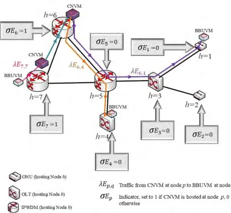
FIGURE 8. CNVM and the traffic toward BBUVMs nodes.

Constraints (24) and (25) ensure that the BBUVMs at nodeh are served by the CNVMs that are hosted at the nodep. Con-straints (26) and (27) determine the location of CNVMs by setting the binary variableσ_pEto 1 if there is a CNVM hosted at node p, whereηis equal to 10−9which is small enough to ensure that the value ofσ_pEis equal to 1 whenP

h∈HλBp,h>0

and ensure σE

p=0 when P

h∈HλBp,h=0. They are

equiv-alent to the logical operation σ_pE=(P

h∈HλBp,h>0?1:0)

explained previously in constraint (23). Fig. 8 illustrates the functions of constraints (26) and (27) whilst Table 5 illus-trates their operation. Constraints (28)–(30) ensure that the CNVMs communicate with each other if they are hosted at different nodespandq, and this is equivalent to the logical operationψp,q=σpE ANDσqE. Fig. 9 illustrates the function

of constraints (28)–(30). Constraints (31) - (38) determine if the hosting node h hosts any VM of any type (BBUVM or CNVM). It is equivalent to the logical operation σ_hχ =

σE

p ANDσqE

6) Communication traffic between CNVMs

λE

p,q= ∇p,q·ψp,q ∀p,q∈H:p6=q (34)

7) Total traffic between two hosting nodes

λT p,q=λ

E p,q+λ

B

p,q ∀p,q∈H:p6=q (35)

8) Flow conservation of the total traffic to the RRH nodes

X

y∈TN x

λR h,r,x,y−

X

y∈TN x

λR h,r,y,x

=   

 

λR

h,r if x = h

−λR

h,r if x = r

0 otherwise

∀r∈R,∀h∈H,∀x∈T (36)

TABLE 5.CNVM constraints operation.

FIGURE 9. CNVM and the common locus.

9) Flow conservation of hosting nodes communication traffic

X

y∈TN x∩H

λT p,q,x,y−

X

y∈TN x∩H

λT p,q,y,x

=   

 

λT

p,q if x = p

−λT

p,q if x = q

0 otherwise

∀p,q,x∈H:p6=q (37)

FIGURE 10. Flow conservation principle.

nodes. Fig. 10 illustrates the principle of flow conservation, and for clarification purposes, it is applied to constraint (36). Constraint (37) represents the flow conservation of the total traffic between any two hosting nodes that might host virtual machines of any type (BBUVM or CNVM).

10) Total BBU workload at any hosting nodeh

9B

h =

X

∀r∈R

λR h,r

! ,

cp· !

9χ ∀h∈H (38)

11) Total normalized workload at hosting nodeh

9i

h+9

f

h=

9B

h +9

C h

.

9S _{∀h∈H (39)}

12) Hosting node capacity

S d·

9i h+σhχ

+9f

h·

S_−S d

≤H

h ∀h∈H (40)

13) GPON link constraints

X

h∈H X

r∈R X

j∈TN i ∩L

λR

h,r,i,j ≤ 0 ∀i∈U (41)

X

p∈H X

q∈H,q6=p X

j∈T_iN∩L

λT

p,q,i,j ≤ 0 ∀i∈U (42)

X

h∈H X

r∈R X

j∈T_iN∩N

λR

h,r,i,j ≤ 0 ∀i∈L (43)

X

p∈H X

q∈H,q6=p X

j∈T_iN∩N

λT

p,q,i,j ≤ 0 ∀i∈L (44)

Constraint (38) represents the total BBU workload at any hosing node h. Constraint (39) calculates the total BBU and CNVM normalized workload at any hosting node. The workload is scaled and normalized relative to the server CPU workload and is separated into integer and fractional parts. Constraint (40) ensures that the total power consumption of hosting VMs does not exceed the maximum power consump-tion allocated for each host. Constraints (41) – (44) ensure

that the total PON downlink traffic does not flow in the opposite direction.

14) Virtual Link capacity of the IP over WDM network

X

p∈H X

q∈H,q6=p

λTp_i,,_jq+X h∈H

X

r∈R

λRh_i,,_jr≤Wi,j·B∀i,j∈N,i6=j.

(45)

15) Flow conservation in the optical layer of IP over WDM network

X

n∈NN m

Wi,j,m,n− X

n∈NN m

Wi,j,n,m

=     

Wi,j if n = i

−Wi,j if n = j

0 otherwise

∀i,j,m∈N,i6=j (46)

Constraint (45) ensures that the total traffic traversing the virtual link (i,j) does not exceed its capacity, in addition it determines the number of wavelength channels that carry the traffic burden of that link. Constraint (46) represents the flow conservation in the optical layer of the IP over WDM net-work. It ensures that the total expected number of incoming wavelengths for the IP over WDM nodes of the virtual link (i,j) is equal to the total number of outgoing wavelengths of that link.

16) Number of wavelength channels

X

i∈N X

j∈N:i6=j

Wi,j,m,n≤w·fm,n ∀m∈N, ∀n∈NmN (47)

17) Total number of wavelength channels

Wm,n= X

i∈N X

j∈N:i6=j

Wi,j,m,n ∀m∈N, ∀n∈NmN (48)

18) Number of aggregation ports

3i= 

 X

j∈L∩TNi 

 X

p∈H X

q∈H,q6=p

λT p,q,i,j

+X

h∈H X

r∈R

λR h,r,i,j

!!

B ∀i∈N (49)

V. MILP MODEL SETUP AND RESULTS

All MILP models were run on high performance computing nodes (HPC) provided through a partnership of the most research-intensive universities in the North of England. The used HPC has four computation modes, the standard mode provides clusters of 252 nodes with up to 6048 cores in total and supports 65 TFLOPS peak using IBM’s iDataPlex hard-ware; and includes a high throughput cluster with 1 GB RAM per nodes, 2900 cores based on twin nodes with 6-core West-mere processors supported by 1GE connectivity between nodes. IBM ILOG CPLEX (12.7) optimization studio is used as an optimization software package where it uses simplex algorithm [47] to solve the developed MILP models.

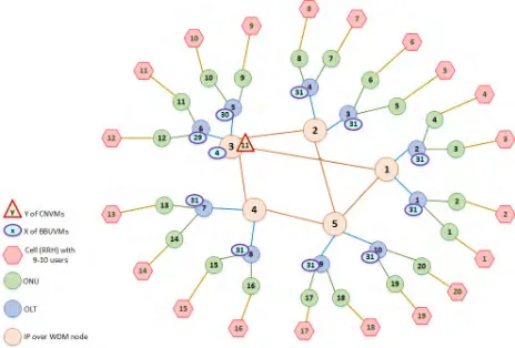
Five IP over WDM nodes are considered constituting the optical backbone network of the proposed architecture. The distribution and topology of the IP over WDM nodes have been built upon the NSFNET network described in [48]–[53]. Each IP over WDM node in turn is attached to two GPONs with one OLT and two ONUs for each GPON. Accord-ingly, the network topology has 10 OLTs and 20 ONUs. In addition, each ONU is connected to one RRH node as shown in Fig. 11. Two GPONs for each IP over WDM node are enough to investigate the VM response for demands and power savings. To finalize the portrait of the network topology, we have concentrated on the distribution of the hosting nodes and the way in which they are connected to each other and for this reason the GPON splitters are not shown.

As alluded to earlier, two types of VMs have been consid-ered: BBUVM, which realizes the functions of the BBU, and CNVM to achieve the functions of the mobile core network. The amount of workload needed for BBUVMs is calculated in GOPS according to (11)[46] and based on the calculated workload, the hosting server CPU utilization due to hosting BBUVMs is determined. On the other hand, the total work-load needed for CNVMs is calculated based on the number BBUVMs group in each hosting node since we have allocated one CNVM for each group of BBUVMs in one hosting node. A single VM consumes around 18W [54] and by knowing the hosting server maximum power consumption 365 (W), idle power 112 (W) and the maximum workload 368 (GOPS),9_hC can calculated for a single VM. Therefore9_hC=corresponds is (18×368)(365−112)=26 (GOPS).

We have investigated the effect of the inter-traffic between CNVMs which is needed to maintain the communication from one side of the network to another such as a call that is held between two mobiles belonging to two different CNVMs. The distribution of CNVMs is sensitive to the inter-traffic flows between them. However, we chose small values for CNVMs inter-traffic in the investigated range. The first value in the range is zero which represents the case where no inter-traffic flows between CNVMs. The maximum value in the range is 16% of the total backhaul traffic which the minimum value at which the MILP model tends to host (pack) all CNVMs at the same node to eliminate the impact of inter-traffic.

FIGURE 11. Tested network topology.

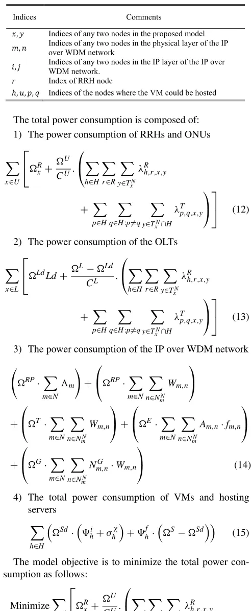
FIGURE 12. Average number of users daily profile [1].

Moving towards the access network, each RRH node is considered to serve a small cell that operates on 10 MHz bandwidth and with a maximum capacity of 10 users. Each user in the small cell is allocated 5 physical resources blocks (PRB) as the users are assumed to request the same task from the network. Accordingly, the total downlink traffic to the RRH node depends on the total number of active users in the small cell. The input parameters to the developed MILP model are listed in Table 6. We have considered 17 time slots over all the day from 00:00 hours to 24:00 hours in steps of 1.5 hours using the average number of users daily profile shown in Fig. 12. The MILP results are compared with the case where there is no NFV deployment. In the ‘‘no virtualization’’ scenario, the BBU is located close to the RRH where they are attached to each other, whilst the integrated platform ASR5000 is deployed to realize mobile core network functionalities and it is connected directly to the IP over WDM network. The ASR5000 maximum power con-sumption, idle power, and maximum capacity are 5760 (W), 800 (W), and 320 (Gbps) respectively [55], whilst the BBU maximum power consumption, idle power, and maximum capacity are 531 (W), 51 (W), 9.8 (Gbps) respectively [56].

TABLE 6. MILP model input parameters.

FIGURE 13. Total power consumption without and with virtualization under different CNVMs inter-traffic at different time slots of a day.

(standard model) as well as the cases where the virtualization is deployed under different CNVMs inter-traffic for different time slots in a day. Fig. 14 shows the total power consumption of the same scenarios versus the total number of active users

FIGURE 14. Total power consumption without and with virtualization under different CNVMs inter-traffic versus total active users in the network.

FIGURE 15. Power saving comparison of virtualization under different CNVMs inter-traffic for a day.

in the networks. The virtualization model has resulted in less power consumption compared to the no virtualization model (standard model) as it optimizes the processing locations of the downlink traffic through optimum placement and consol-idation of VMs.

Fig. 15 compares the total power saving of the virtualiza-tion model under different CNVMs inter-traffic for one day while Fig. 16 show the virtualization power saving under different CNVMs inter-traffic versus total number of active users. Compared to other virtualization cases, virtualization without CNVMs inter-traffic has saved a maximum of 38% (average 34%). This is because there is no power consumed by the CNVMs inter-traffic as this traffic is zero. The total power saving decreases as the CNVMs inter-traffic increases to reach its lowest value in the case of virtualization with 16% CNVMs inter-traffic which is 37% (average 32%).

FIGURE 16. Power saving comparison of virtualization under different CNVMs inter-traffic versus total number of active users.

FIGURE 17. 3-Dimensional presentation of the total power saving for virtualization under different CNVMs inter-traffic versus different number of active users in the network.

CNVMs inter-traffic produces relatively small amount of power consumption compared to the power consumption induced by the fronthaul traffic and hosting server as shown in Fig. 17. As the inter-traffic increases, the MILP model tends to eliminate its effect by consolidating CNVMs in one place.

Although virtualization has saved a maximum of 38% (without CNVMs inter-traffic) and 37% (with 16% CNVMs inter-traffic) of the total power consumption, it cannot pro-vide such level of power saving over the entire day. As the number of active users varies with the time of day (as in Fig. 12), the power saving achieved by virtualization varies accordingly. The results in Figs. 15 and 16 show that a high-power saving is achieved when the total number of active users is around 20% (around 4 am to 8 am) while the lowest power saving is recorded at high number of active users (during the day rush hours). At small number of active users, the MILP model tends to consolidate all the VMs in the IP over WDM network to minimize the number of servers hosting VMs to reduce the total power consumption.

FIGURE 18. VMs distribution over network under active users 13% of the total network capacity without CNVMs inter-traffic.

FIGURE 19. VMs distribution over network under active users 13% of the total network capacity and 16% CNVMs inter-traffic.

Figs. 18 and 19 show the VMs consolidation and dis-tribution over the network at low number of active users (13%) under CNVMs of 0% and 16% respectively. At low number of active users and 0% inter-traffic, the MILP model consolidates the VMs at the IP over WDM network. Since the total number of active users is low, the fronthaul traffic is relatively low and consequently the power consumption induced by the fronthaul traffic is low compared to the host-ing power consumption (servers power). For this reason, the MILP model tends to pack BBUVMs in the IP over WDM network as much as possible to reduce the power consumed by the hosting servers. Also, the MILP model tends to host CNVMs close to the BBUVMs as the inter-traffic between CNVMs is zero. Once the inter-traffic is greater than zero, the MILP model consolidates the CNVMs at one location as in Fig. 19.

FIGURE 20. VMs distribution over network under active users 100% of the total network capacity without CNVMs inter-traffic.

FIGURE 21. VMs distribution over network under active users 100% of the total network capacity and 16% CNVMs inter-traffic.

to the users which are the OLTs, while CNVMs inter-traffic has no effect on the distribution of BBUVMs.

Hosting BBUVMs in OLTs when the number of users is high ensures shorter paths for the fronthaul traffic than hosting BBUVMs in the IP over WDM networks and con-sequently, the power consumed by this traffic is less. For CNVMs, the MILP model tends to distribute them close to the BBUVM when there is no inter-traffic between them, and this is clearly seen in Fig. 20. In contrast, when the inter-traffic between CNVMs is greater than zero, the MILP model tends to centralize the location of CNVMS in the IP over WDM network to reduce the power consumption induced by the inter-traffic and the power of the hosting servers as shown in Fig. 21.

VI. REAL-TIME HEURISTICS IMPLEMENTATION AND RESULTS

A. ENERGY EFFICIENT NFV WITH NO CNVMs INTER-TRAFFIC (EENFVnoITr) HEURISTIC

The EENFVnoITr provides real-time implementation of the MILP model without CNVMs inter-traffic. The pseudocode

Algorithm 1Energy Efficient NFV without CNVMs inter-traffic (EENFVnoITr) Heuristic

INPUT:G=(NE,L),Gp=(N,Lp)

OUTPUT:VMs location, workloads, and distribution

1: ∀_r ∈ _RRH determine number of users and calculate node demand (rDr); where Dr ∈ D /∗D is the total

demands∗/

2: ∀Dr ∈Ddetermine BBUVM workload9r

3: ∀r∈RRHfind

(r,h)=min(shortestPath(r,{h∈NE∩OLT})

4: iftotal workload ofh>> 9r

5: host BBUVM inh 6: update workload ofh

7: Dr ∈Dserved

8: end if

9: ∀Dr ∈/ Dserved find (r,h) =

min(shortestPath(r,{_h∈N})) /∗ where N is the IP over WDM nodes∗/

10: host BBUVM inh 11: update workload ofh

12: Dr ∈Dserved

13: Route the fronthaul traffic from BBUVMs to RRH nodes 14: N0 ←DESCENDSORT(N) and seti=1

15: Host CNVM inN0(i),N0(i−1),. . .N0(1) 16: ∀CNVM in n∈N0and∀BBUVM in h∈NE

find (n,h)=min(shortest Path(n,h)) 17: Route the traffic from CNVMs to BBUVMs 18: Determine the IP over WDM network configuration 19: ifi=1

20: Determine total power consumption as (minTPC) 21: end if

22: Determine the total power consumption as TPC(i) 23: ifminTPC≥TPC(i)

24: minTPC=TPC(i) 25: i=i+1

26: goto 15 27: else

28: minimum power consumption isminTPC 29: EXIT

30: end if

of the heuristic is shown in Algorithm 1. The network is modelled by sets of network elementsNE, and linksL. The heuristic obtains the network topologyG =(NE,L) and the physical topology of the IP over WDM networkGp=(N,Lp)

whereN is the set of IP over WDM nodes andLpis the set of

a way that it serves as many RRH requests as possible. The EENFVnoITr heuristic may host a BBUVM in an OLT node if it has enough processing capacity to serve all the requests from the closest RRH nodes. In this way, the heuris-tic exploits bin packing techniques to reduce the processing power consumption. The amount of fronthaul traffic delivered by each BBUVM determines the backhaul traffic flows from each CNVMs toward BBUVMs. The EENFVnoITr heuristic determines the total amount of backhaul traffic that may flow from each IP over WDM node and sorts them in a descending order. The nodes in the top of the sorted list of IP over WDM nodes represent highly recommended nodes to host CNVMs. In such a scenario, the EENFVnoITr heuristic ensures less of the backhaul traffic flows in the IP over WDM network. The EENFVnoITr heuristic uses the sorted list to accommodate CNVMs. Once the VMs are distributed and the logical traffic is routed, the EENFVnoITr heuristic obtains the physical graphGp = (N,Lp) and determines the traffic in each

net-work segment. The IP over WDM netnet-work configuration such as the number of fibers, router ports, and the number of EDFA is determined the total power consumption is evaluated. The heuristic algorithm continuously increases the number of CNVMs candidate locations by one, re-configures the IP over WDM network, and re-evaluates the power consumption and compare it to the power consumption in the previous iteration until it determines the best number and location of CNVMs for minimum power consumption. The heuristic model

B. ENERGY EFFICIENT NFV WITH CNVMs INTER-TRAFFIC (EENFVwithITr) HEURISTIC

This section describes the energy efficient NFV with CNVMs inter-traffic heuristic (EENFVwithITr). The EENFVwithITr heuristic extends the EENFVnoITr heuristic to provide real-time implementation of the MILP model where the CNVMs are considered. The pseudocode of the heuristic is shown in algorithm 2. It uses the same approach used by EENFVnoITr, but it evaluates the CNVMs inter-traffic after the locations of CNVMs are determined.

C. EENFVnoITr AND EENFVwithITr HEURISTICS RESULTS

In order to verify the results of the proposed MILP model, the network topology in Fig. 11 used for the MILP model is also used to evaluate the heuristics. All the parameters considered in the MILP model such as the wireless band-width, number of resources blocks per user, and the param-eters in Table 6 are considered in the evaluation of both EENFVnoITr and EENFVwithITr heuristics. The number of users allocated to each cell in the heuristics is the same as in the MILP model to ensure the requested traffic by each RRH node is the same in all models. Fig. 22 compares the total power consumption of MILP with EENFVnoITr model at different times of the day when the CNVMs inter-traffic is not considered. It is clearly seen that there is a small difference in the total power consumption of the two models and it varies over the day according to the total number of active users. The total power consumption of the MILP model is less than

Algorithm 2 Energy Efficient NFV With CNVMs Inter-Traffic (EENFVwithITr) Heuristic

INPUT:G=(NE,L),Gp=(N,Lp)

OUTPUT:VMs location, workloads, and distribution

1: ∀_r∈_RRHdetermine number of users and calculate node demand (rDr); whereDr ∈D/∗Dis the total demands∗/

2: ∀Dr ∈Ddetermine BBUVM workload9r

3: ∀r ∈ RRH find (r,h) =

min(shortestPath(r,{h∈NE∩OLT})

4: iftotal workload ofh>> 9r

5: host BBUVM inh 6: update workload ofh

7: Dr ∈Dserved

8: end if

9: ∀Dr ∈/ Dserved find (r,h) =

min(shortestPath(r,{h∈N})) /∗ where N is the IP over WDM nodes∗/

10: host BBUVM inh 11: update workload ofh

12: Dr ∈Dserved

13: Route the fronthaul traffic from BBUVMs to RRH nodes

14: N0 ←DESCENDSORT(N) and seti=1

15: Host CNVM inN0(i),N0(i−1),. . .N0(1) 16: ∀CNVMinn∈N0and∀BBUVMinh∈NE

find(n,h)=min(shortestPath(n,h)) 17: Route the traffic from CNVMs to BBUVMs 18: ∀CNVMinnxny ∈ N

0

;x 6= y find nx,ny

=

min shortestPath nx,ny

19: Route the traffic from CNVMs to CNVMs

20: Determine the IP over WDM network configuration 21: ifi=1

22: Determine total power consumption as (minTPC) 23: end if

24: Determine the total power consumption as TPC(i) 25: ifminTPC≥TPC(i)

26: minTPC=TPC(i) 27: i=i+1 28: goto 15 29: else

30: minimum power consumption isminTPC 31: EXIT

32: end if

FIGURE 22. Total power consumption of MILP with without CNVMS inter-traffic compared with EENFVnoITr heuristic model.

FIGURE 23. VM servers power consumption of MILP model compared with EENFVnoITr heuristic.

the VM servers are met, the heuristic accommodates a CNVM in the server. This case results in high EENFVnoITr VM server power consumption compared with MILP model. This is clearly seen in Fig. 23 where the VM servers power con-sumption of the MILP model and the EENFVnoITr heuristic are compared. The total network power consumption of both EENFVnoITr heuristic and the MILP model are the same for most of the time of the day. Fig. 24 shows the net-work power consumption of the MILP model compared with EENFVnoITr heuristic.

It shows that there is a small difference in the network power consumption between the two models during the time of the day when the total number of active users is low. This is driven by the approach of the MILP model where it tends to accommodate the CNVMs at the IP over WDM nodes rather than OLT at the time of the day where the total number of users is low. In contrast, the heuristic tends to accommodate the CNVMs wherever the VM server is close to the BBUVMs and it has enough capacity. Fig. 25 compares the total power consumption of EENFVwithITr with the MILP model when the CNVMs inter-traffic is 16% of the total backhaul traffic. It is clearly seen that there is a small difference in the total

FIGURE 24. Network power consumption of MILP model compared with EENFVnoITr heuristic.

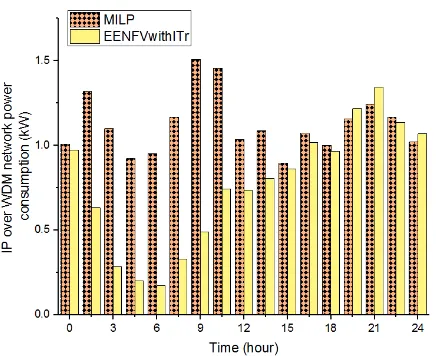
FIGURE 25. Total power consumption of MILP model compared with EENFVwithITr heuristic at CNVMs inter-traffic 16% of the total backhaul traffic.

FIGURE 26. IP over WDM network power consumption of MILP model compared with EENFVwithITr heuristic at CNVMs inter-traffic 16% of the total backhaul traffic.

FIGURE 27. VM servers power consumption of MILP model compared with EENFVwithITr heuristic at CNVMs inter-traffic 16% of the total backhaul traffic.

their location, and available capacity increases the processing distribution of VMs in the network which leads to a high VM servers power consumption compared with the MILP model as shown in Fig. 27 which compares the VM servers power consumption of the MILP model with EENFVwithITr heuristic during different times of the day.

D. COMPLEXITY ANALYSIS

Both EENFVnoITr and EENFVwithITr heuristic algorithms were developed to tackle the non-deterministic-polynomial time hardness (NP-hard) problem of the linear programming model proven in [67]. Two main processes form the core of both heuristics: hosting VMs in the network nodes and routing the traffic between VMs; and between VMs and RRH nodes. Hosting VMs in network nodes is done in two stages: hosting BBUVMs and hosting CNVMs. To host BBUVMs in the network nodes, two nested loops are needed with (R×N) iterations where R is the number of RRH nodes and N is the number of hosting nodes, while (N×N=N2) iterations are needed to host the CNVMs. As the number of users increases,

FIGURE 28. VM servers power consumption of MILP model compared with EENFVwithITr heuristic at CNVMs inter-traffic 16% of the total backhaul traffic.

the network size increases and the number of RRH nodes will be approximately equal to the number of hosting nodes N (R = N). However, hosting VMs in the network nodes has complexity of (Big O) O(k ×N2) time, where k is a constant equals to 2. On the other hand, routing the traffic between VMs and also between VMs and RRH nodes is based on the minimum hop algorithm which has complexity of order O(N) [68]. Thus, the overall time complexity is a polynomial time complexity expressed as O kN2+O(N). However, EENFVnoITr and EENFVwithITr algorithms time complexity is approximately O N2as it is the dominant term in the aforementioned complexity expression. EENFVnoITr and EENFVwithITr algorithms running time versus the net-work size is shown in Fig. 28 where it is evaluated up to 2000 users. The results in Fig. 28 were obtained when the EENFVnoITr and EENFVwithITr algorithms were executed in an Intel Core i5, 3.00 GHz processor with 16 GB RAM.

VII. GENETIC ALGORITHM IMPLEMENTATION

In this section, a genetic algorithm (GA) is introduced as an alternative approach to validate the results. The main differ-ence between EENFVnoITr and EENFVwithITr algorithms is the added consideration of the traffic between CNVMs carried out by EENFVwithITr where this traffic is considered zero in EENFVnoITr. The genetic algorithm is developed here for the case where traffic flows between CNVMs which is the general case, thus avoiding redundant verification of the results.

The principle of GA is to let a certain population of several candidates or individuals to evolve through a number of gen-erations in the search of the individual that has the optimum fitness. The optimum fitness in this work is the minimum.

FIGURE 29. BBUVMs chromosome structure.

FIGURE 30. CNVMs chromosome structure.

The first step in the GA is to define chromosomes for the problem under study. Two types of chromosomes are defined in this work: BBUVMs chromosome, and CNVMs chromosome. The BBUVMs chromosome has 700 genes corresponding to the binary decision (σ_hrB) that is introduced in the MILP model. Each gene represents a BBUVM hosted in a specific node to serve an RRH node. If the hosting node h1 has a BBUVM that serves a RRH node r1 then the corre-sponding gene is set to 1, otherwise it is set to zero. A two dimensional array representation of BBUVM chromosome is shown in Fig. 29.

The same methodology is applied to construct the CNVMs chromosome. The CNVMs chromosome has 175 genes where each gene represents a CNVM at an IP over WDM node that serves a BBUVM at a specific hosting node. If a node h2 has a CNVM that serves a BBUVM at node h5 then the corresponding chromosome is set to 1. Otherwise, it is set to zero. The two dimensional array representation of CNVMs chromosome is shown in Fig. 30.

The fitness function in the developed algorithm consists of evaluating the power consumption associated with traffic routing and VM processing for each individual. After that selection, crossover, and mutation are applied to create a new generation of individuals as shown in Algorithm 3.

A. GA SETUP AND RESULTS

We have considered two types of chromosomes: BBUVMs chromosome and CNVMs chromosome. The

Algorithm 3 Energy Efficient NFV With CNVMs Inter-Traffic (EENFVwithITr) Heuristic

INPUT:initial populations

OUTPUT:minimum power consumption

1: Set a counter for the number of generationi=1 2: Get the initial population

3: Evaluation of the population fitness 4: Select parents

5: Crossover 6: Mutation 7: Elitism

8: Get a new population

9: if the termination criteria is not satisfied 10: i=i+1

11: goto 3 12: else

13: Optimal Power Consumption 14: EXIT

15: end if

FIGURE 31. Fitness history.

BBUVMs chromosome has 700 genes corresponding to 35 candidates that can host BBUVM (ONU+OLT+IP over WDM nodes) multiplied by 20 RRH nodes as proposed in the topology used. CNVMs chromosome has 175 genes corresponding to 5 candidates IP over WDM nodes to host CNVMs multiplied by 35 candidates to host BBUVMs. We have considered 10 chromosomes for each type (BBU-VMs and CN(BBU-VMs) to be evolved throughout 100 generations with probabilities of crossover 95%, mutation 0.01% and elitism 20%. The fitness function (power consumption) was recorded at each generation and is illustrated in Fig. 31. The fitness history graph shows that the solution (minimum power consumption) is obtained beyond generation 65 where the graph shows no further change.

FIGURE 32. Total power consumption of GA compared with EENFVwithITr heuristic and MILP model at CNVMs inter-traffic 1% of the total backhaul traffic.

CNVMs inter-traffic 1% of the total backhaul traffic. The results are illustrated in Fig. 32 and they are comparable.

VIII. CONCLUSIONS

This paper has investigated network function virtualization in 5G mobile networks with the impact of total number of active users in the network, the backhaul/fronthaul configu-rations, and the inter-traffic between VMs. A MILP optimiza-tion model was developed with the objective of minimizing the total power consumption by optimizing the VMs loca-tions and VM servers’ utilization. The MILP model results have been investigated under the impact of CNVMs traffic variation, and variation in the total number of active users during different times of the day. The MILP model results show that virtualization can save up to 38% (average 34%) of the total power consumption, also the results reveal how the total number of active users affects the BBUVMs distri-bution while CNVMs distridistri-bution is affected mainly by the inter-traffic between them. For real-time implementation, this paper has introduced two heuristics: Energy Efficient NFV without CNVMs inter-traffic and Energy Efficient NFV with CNVMs inter-traffic. The results obtained through the use of the heuristics were compared with the MILP model results. The comparisons showed that the total power consumption when the heuristics are used is higher than the total power consumption when the MILP optimization model is used by a maximum of 9% (average 5%). Finally, a Genetic algorithm has been introduced to for further results verification.

ACKNOWLEGMENT

The authors would like to acknowledge them for funding this work. Mr. Ahmed Al-Quzweeni would like to acknowledge HCED for funding his Ph.D. All data are provided in full in the results section of this paper.

REFERENCES

[1] G. Aueret al., ‘‘How much energy is needed to run a wireless network?’’

IEEE Trans. Wireless Commun., vol. 18, no. 5, pp. 40–49, Oct. 2011. [2] Cisco Visual Networking Index: Forecast and Methodology 2016–2021,

Cisco, San Jose, CA, USA, Jun. 2017.

[3] I. Neokosmidis, T. Rokkas, P. Paglierani, C. Meani, K. M. Nasr, and K. Moessner, ‘‘Techno economic assessment of immersive video services in 5G converged optical/wireless networks,’’ inProc. Opt. Fiber Commun. Conf. Expo. (OFC), Mar. 2018, pp. 1–3.

[4] V. G. Nguyenet al.,A Comprehensive Guide to 5G Security, 1st ed. Hoboken, NJ, USA: Wiley, 2018, pp. 31–57.

[5] Z. Zhang, Y. Gao, Y. Liu, and Z. Li, ‘‘Performance evaluation of shortened transmission time interval in LTE networks,’’ in Proc. IEEE Wireless Commun. Netw. Conf. (WCNC), Apr. 2018, pp. 1–5.

[6] L. Belkhir and A. Elmeligi, ‘‘Assessing ICT global emissions foot-print: Trends to 2040 & recommendations,’’J. Cleaner Prod., vol. 177, pp. 448–463, Mar. 2018.

[7] A. Z. Aktas, ‘‘Could energy hamper future developments in information and communication technologies (ICT) and knowledge engineering?’’

Renew. Sustain. Energy Rev., vol. 82, pp. 2613–2617, Feb. 2018. [8] P. Liu, G. Xu, K. Yang, K. Wang, and X. Meng, ‘‘Jointly optimized

energy-minimal resource allocation in cache-enhanced mobile edge computing systems,’’IEEE Access, vol. 7, pp. 3336–3347, 2019.

[9] P. Lähdekorpi, M. Hronec, P. Jolma, and J. Moilanen, ‘‘Energy efficiency of 5G mobile networks with base station sleep modes,’’ inProc. IEEE Conf. Standards Commun. Netw. (CSCN), Sep. 2017, pp. 163–168.

[10] X. Ge, J. Yang, H. Gharavi, and Y. Sun, ‘‘Energy efficiency challenges of 5G small cell networks,’’IEEE Commun. Mag., vol. 55, no. 5, pp. 184–191, May 2017.

[11] R. Bassoli, M. Di Renzo, and F. Granelli, ‘‘Analytical energy-efficient planning of 5G cloud radio access network,’’ inProc. Proc. IEEE Int. Conf. Commun. (ICC), May 2017, pp. 1–4.

[12] K. Zhanget al., ‘‘Energy-efficient offloading for mobile edge computing in 5G heterogeneous networks,’’IEEE Access, vol. 4, pp. 5896–5907, 2016. [13] J. G. Andrewset al., ‘‘What will 5G be?’’IEEE J. Sel. Areas Commun.,

vol. 32, no. 6, pp. 1065–1082, Jun. 2014.

[14] T. Choi, T. Kim, W. TaverNier, A. Korvala, and J. Pajunpaa, ‘‘Agile management of 5G core network based on SDN/NFV technology,’’ inProc. Int. Conf. Inf. Commun. Technol. Converg. (ICTC), Oct. 2017, pp. 840–844. [15] H. Hawilo, L. Liao, A. Shami, and V. C. M. Leung, ‘‘NFV/SDN-based vEPC solution in hybrid clouds,’’ inProc. IEEE Middle East North Africa Commun. Conf. (MENACOMM), Apr. 2018, pp. 1–6.

[16] S. H. Wonet al., ‘‘Development of 5G CHAMPION testbeds for 5G services at the 2018 Winter Olympic Games,’’ inProc. IEEE 18th Int. Workshop Signal Process. Adv. Wireless Commun. (SPAWC), Jul. 2017, pp. 1–5.

[17] V. Q. Rodriguez and F. Guillemin, ‘‘Cloud-RAN modeling based on paral-lel processing,’’IEEE J. Sel. Areas Commun., vol. 36, no. 3, pp. 457–468, Mar. 2018.

[18] G. C. Valastro, D. Panno, and S. Riolo, ‘‘A SDN/NFV based C-RAN architecture for 5G mobile networks,’’ inProc. Int. Conf. Sel. Topics Mobile Wireless Netw. (MoWNeT), Jun. 2018, pp. 1–8.

[19] A. Tzanakakiet al., ‘‘Wireless-optical network convergence: Enabling the 5G architecture to support operational and end-user services,’’IEEE Commun. Mag., vol. 55, no. 10, pp. 184–192, Oct. 2017.

[20] M. Rivaet al., ‘‘An elastic optical network-based architecture for the 5G fronthaul,’’ inProc. Simpósio Brasileiro Redes Comput. (SBRC), 2018, pp. 1–11.

[21] J. Luo, Q. Chen, and L. Tang, ‘‘Reducing power consumption by joint sleeping strategy and power control in delay-aware C-RAN,’’IEEE Access, vol. 6, pp. 14655–14667, 2018.

[22] 3GPP.Releases. Accessed: Mar. 3, 2016. [Online]. Available: http://www. 3gpp.org/specifications/67-releases.

[23] C. D. Monfreid. (2012). The LTE Network Architecture– A Comprehensive Tutorial. Alcatel-Lucent, Paris, France. Accessed: Oct. 11, 2018. [Online]. Available: http://www.cse.unt.edu/∼rdantu/FALL _2013_WIRELESS_NETWORKS/LTE_Alcatel_

White_Paper.pdf

[24] Alcatel-Lucent. Interworking LTE EPC With W-CDMA Packet Switched Mobile Cores. Accessed: Sep. 20, 2017. [Online]. Available: http://www.alcatel-lucent.com

[25] A. Al-Quzweeni, T. E. H. El-Gorashi, L. Nonde, and J. M. H. Elmirghani, ‘‘Energy efficient network function virtualization in 5G networks,’’ pre-sented at the 17th Int. Conf. Transparent Opt. Netw. (ICTON), Jul. 2015. [26] A. Al-Quzweeni, A. Lawey, T. El-Gorashi, and J. M. H. Elmirghani,

‘‘A framework for energy efficient NFV in 5G networks,’’ inProc. 18th Int. Conf. Transparent Opt. Netw. (ICTON), Jul. 2016, pp. 1–4. [27] M. H. Alsharif and R. Nordin, ‘‘Evolution towards fifth generation (5G)