group object tracking with irregular shapes
.
White Rose Research Online URL for this paper:
http://eprints.whiterose.ac.uk/140444/
Version: Accepted Version
Article:
Aftab, W., Hostettler, R., De Freitas, A. et al. (2 more authors) (2019) Spatio-temporal
Gaussian process models for extended and group object tracking with irregular shapes.
IEEE Transactions on Vehicular Technology. ISSN 0018-9545
https://doi.org/10.1109/TVT.2019.2891006
© 2019 IEEE. Personal use of this material is permitted. Permission from IEEE must be
obtained for all other users, including reprinting/ republishing this material for advertising or
promotional purposes, creating new collective works for resale or redistribution to servers
or lists, or reuse of any copyrighted components of this work in other works. Reproduced
in accordance with the publisher's self-archiving policy.
[email protected] https://eprints.whiterose.ac.uk/
Reuse
Items deposited in White Rose Research Online are protected by copyright, with all rights reserved unless indicated otherwise. They may be downloaded and/or printed for private study, or other acts as permitted by national copyright laws. The publisher or other rights holders may allow further reproduction and re-use of the full text version. This is indicated by the licence information on the White Rose Research Online record for the item.
Takedown
If you consider content in White Rose Research Online to be in breach of UK law, please notify us by
Spatio-temporal Gaussian Process Models for
Extended and Group Object Tracking with Irregular
Shapes
Waqas Aftab, Roland Hostettler,
Member, IEEE
, Allan De Freitas, Mahnaz Arvaneh,
and Lyudmila Mihaylova,
Senior Member, IEEE
Abstract—Extended object tracking has become an integral part of many autonomous systems during the last two decades. For the first time, this paper presents a generic spatio-temporal Gaussian process (STGP) for tracking an irregular and non-rigid extended object. The complex shape is represented by key points and their parameters are estimated both in space and time. This is achieved by a factorization of the power spectral density function of the STGP covariance function. A new form of the temporal covariance kernel is derived with the theoretical expression of the filter likelihood function. Solutions to both the filtering and the smoothing problems are presented. A thorough evaluation of the performance in a simulated environment shows that the proposed STGP approach outperforms the state-of-the-art GP extended Kalman filter approach [1], with up to90%improvement in the accuracy in position,95%in velocity and7%in the shape, while tracking a simulated asymmetric non-rigid object. The tracking performance improvement for a non-rigid irregular real object is up to 43%in position,68%in velocity,10%in the recall and 115%in the precision measures.
Index Terms—Extended Object Tracking, Spatio-temporal Gaussian Process, Rauch-Tung-Streibel Smoother.
I. INTRODUCTION
E
XTENDED object tracking (EOT) includes the process of estimating the kinematic states and the shape parameters of the objects of interest using a sequence of noisy sensor measurements. Group object tracking (GOT) involves state estimation of closely spaced objects moving with similar dynamics. Often, the average dynamics and the shape of the group are estimated over time. Since the state estimation requirements are comparable, hence the methods for EOT and GOT are similar. EOT and GOT are an integral part of various autonomous systems1, for example: robot navigation [2], people tracking using depth sensors such as Microsoft Kinect [3]. Other applications include crowd analysis [4], tracking of chemical, biological, radiological and nuclear (CBRN) pollutant clouds [5] and sea surveillance [6]. In all these systems, specialized sensors are used to collect measurements. AlthoughCopyright (c) 2015 IEEE. Personal use of this material is permitted. However, permission to use this material for any other purposes must be obtained from the IEEE by sending a request to [email protected].
W. Aftab, M. Arvaneh, L. Mihaylova and A. De Freitas are at the Department of Automatic Control and Systems Engineering (ACSE), The University of Sheffield, Sheffield, UK. waftab1,m.arvaneh,[email protected]. [email protected]
R. Hostettler is at the Department of Electrical Engineering and Automation, Aalto University, Espoo, Finland. [email protected].
1From here on, the term EOT is used only and everything proposed in this
paper is applicable to the GOT as well.
the states are interpreted according to the application, the measurement processing and the state estimation requirements are similar. The object kinematic states such as the position, velocity or other higher order time derivatives and shape parameters are estimated based on sensor data. The shape is generally represented by the size or volume parameters.
The EOT methods are also applied in self-driving cars navi-gating through the urban traffic [7]. Although the technology of autonomous vehicles has many advantages, the main focus is on improving safety and resilience of this technology. Various types of sensors, such as a camera, radar and LiDAR (light detection and ranging), are installed for detection and tracking of roads and obstacles [8]–[10], around the driverless car. The EOT techniques are an inherent part of the cars obstacle avoidance and navigation system.
Tracking multiple point objects (commonly called targets) is known as multi-target tracking (MTT) [11], [12] and requires non-linear estimation methods that successfully deal with data association and clutter. In contrast to tracking point targets [13]– [16], which has been a widely researched area, EOT is a relatively new area and has seen an increase in real-world applications during the last two decades. In point objects tracking, the object kinematics is estimated and most methods assume single measurement per object per time sample. In a similar way, in EOT, the kinematics as well as the shape, extent, and size of the object are estimated. Moreover, multiple measurements per object per time sample are received. The already developed kinematics models for point objects [17], [18] have been typically used in the EOT kinematic state estimation. Hence, the focus of the EOT research has been on the measurement models, the shape estimation and data association.
A Gaussian Process (GP) [20] can also be employed for estimation of the extent. A GP is a distribution over an unknown and nonlinear function, in the continuous domain. The observed values of these functions can be used to predict the values at unobserved points. Traditionally, the GP is a batch processing method and cannot be used for real-time applications. A GP based recursive filter for real-time EOT has been proposed in [1], [21]. This GP based EOT method models the correlations in a single input domain. The extent states consist of radial values of the object extent from the CoO at different angles. The GP is used to model the nonlinear mapping of the spatial input (angle) to the spatial output (radius). However, the spatial output is correlated in both the spatial and the temporal domain. In [22], it has been shown that if one of the input dimensions is stationary (and some other conditions), then it has an equivalent state space representation which can be solved using Rauch-Tung-Streibel smoothing. The model is termed as spatio-temporal GP (STGP). A recursive equivalent of a temporal GP is proposed in [23], [24] and of an STGP is proposed in [22]. The filter requires a forward pass and is suitable for a real-time implementation. The smoother requires a forward and backward pass and the increase in computational expense with time makes it unsuitable for real-time processing. In this paper, a new model based on the recursive equivalent of the STGP is proposed for real-time tracking of a non-rigid extended object.
A. Related Work
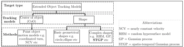
Recent methods for EOT have been comprehensively summa-rized in two overview papers [15] and [16]. The EOT research can be divided into two parts as shown in Fig. 1: tracking of the CoO and the shape. The CoO kinematics models have been inherited and are similar to the point object kinematics models. Object shapes have been estimated using basic geometric shapes based models for example stick [25], circle [26], [27], rectangle [28] or ellipse [13], [29]. Although the real world objects do not typically have such basic geometrical shapes, these models have been shown to perform satisfactorily well in some applications such as tracking boats with elliptical shapes [30] or cars with rectangular shapes [31]. In the presence of sensor clutter and multiple objects or for tracking irregularly shaped objects, a more detailed shape estimation not only improves the data association performance by providing more accurate confidence regions but also gives better kinematics states estimation [16]. Relatively complex shape models have been proposed using a mixture of ellipsoids [32] or star-convex shape models such as random hypersurface model (RHM) [33] and GP model [1]. The shape changes have been estimated well using basic geometrical shape models. These models are however insufficient for the tracking of irregularly shaped objects. The shape changes in the complex shape models, which perform better for irregular shapes, and some other basic shape models such as the random matrix approach the shape is assumed constant (rigid) and the changes in the shape are incorporated using motion process noise (random walk) [13], [14], [34]. A different approach is taken in the GP extended Kalman filter (GP-EKF) [1], where the
shape changes are modeled using a forgetting factor. When tracking non-rigid extended objects, the extent changes over time. Tracking performance is degraded in such scenarios when modeled using the random walk or a forgetting factor shape change model. Additionally, in [1] the GP based approach has been proposed equivalent to a batch GP regression without giving the theoretical explanation and the necessary conditions for the equivalence. Additionally, the measurement noise is ignored at some points during the derivation of the measurement likelihood.
B. Contributions
The contribution area of the proposed model in the EOT literature is depicted in Fig. 1. The key contributions of this work are as follows; (i) A novel interpretation of the center of an asymmetric extended object is presented (given in Subsection IV-A). (ii) A novel non-rigid extended object tracker is proposed based on an STGP model, which includes both the spatial and the temporal correlations of the extent (See Subsection IV-C). (iii) Based on the theoretical results of [22], the full GP regression is proposed to be approximated using a fixed-lag Rauch-Tung-Streibel smoother to obtain quasi-real time approach. This is the first time in the literature of EOT that the theoretical fundamentals of the equivalence between a batch and the recursive GP regression are described for deep understanding (See Subsection IV-H). (iv) A real-time fixed lag smoother based on the STGP model is proposed, which improves upon the accuracy of the filter estimates (See Subsections IV-H and VI-B). (v) The measurement likelihood is derived considering all noises. Due to the complex relationship between the states and the measurements, the previous GP based implementations of the EOT ignored part of the noise (given in Subsection IV-E). (vi) The performance validation of the proposed approach is provided on real and simulated data. The computational complexity and the effect of smoother lag is also evaluated (given in Section VI).
The remaining part of the paper is structured as follows. The theoretical background of the GP and the STGP is covered in Section II and that of inference is covered in Section III. The proposed model of the EOT is explained in Section IV, an example is given in Section V and the evaluation is presented in Section VI followed by conclusions. The sensor measurements coordinate conversions are given in Appendix A and the transformed sensor noise pdfs are derived in Appendix B.
II. GAUSSIANPROCESSREGRESSIONMODELS A. Gaussian Processes
Extended Object Tracking Models
Center of object
(CoO) Shape
Basic geometrical shapes e.g. circle,ellipse etc
Complex shapes e.g. RHM, GP,
STGPetc Point object
motion models e.g. coordinated turn,
NCV etc
Target type
Tracking models
Methods
NCV = nearly constant velocity RHM = random hypersurface model GP = Gaussian process
[image:4.612.123.489.54.148.2]STGP = spatio-temporal Gaussian process Abbreviations
Fig. 1. The proposed innovation. The figure gives a hierarchical representation of single EOT research and highlights the contribution of this paper within this paradigm. A complex extent model namely STGP (bold) has been proposed in this paper.
can predict the mean output and its uncertainty at new input locations.
Suppose a GP models the nonlinear functiongfrom a random inputθ to an output γgiven below:
γ=g(θ), g(θ)∼GP(µ(θ), k(θ, θ′)), (1) where µ(θ) represents the mean and k(θ, θ′) represents the covariance kernel of the GP. The output γ is observed atn
different input values and modeled using the measurement equation given below:
z=g(θ) +v, (2)
wherez= [z1, z2, ..., zn]T represents the measurement vector
corresponding to the input vectorθ= [θ1, θ2, ..., θn]T,g(θ) =
[g(θ1), g(θ2), ..., g(θn)]T represents the function values vector,
v ∼ N(0, σ2I
n)represents the additive independent identically
distributed (i.i.d.) measurement noise vector with variance σ2 and In represents ann-dimensional identity matrix. Several
works on GP regression for non-i.i.d. Gaussian measurement noise assumption can be found at [35]–[37]. The GP covariance matrixΣθθand the GP prediction at the new input vectorθ⋆
is given below [20]:
Σθθ=
k(θ1, θ′1) k(θ1, θ′2) · · · k(θ1, θ′n)
..
. ... . .. ...
k(θn, θ1′) k(θn, θ′2) · · · k(θn, θn′)
, (3)
µ(θ⋆) =µ(θ) +Σθ⋆θ(Σθθ+σ2In)−1[g(θ)−µ(θ)], (4)
C(θ⋆) =Σθ⋆θ⋆−Σθ⋆θ(Σθθ+σ2In)−1Σθθ⋆, (5)
whereµ(θ)represents the mean vector of GP atθ,µ(·)and C(·) represent, respectively, the mean vector and the error covariance matrix of the GP prediction.
B. Spatio-Temporal Gaussian Processes
An STGP is a stochastic process model for systems evolving in both space and time [22]. Let the spatial input be represented byθand the temporal input is represented byt, then an STGP can be used to model a functional mapping from the input to the outputr of the form given below:
r=f(θ, t), f(θ, t)∼ST GP(µ(θ, t), k(θ, θ′;t, t′)), (6) whereµ(θ, t)andk(θ, θ′;t, t′)represent, respectively, the mean
and the covariance kernel of the STGP model. The STGP regression can be determined in the same way as the GP regression explained in Subsection II-A. The time complexity of determining an STGP regression on a model trained atT
time steps for N input locations is O(N3T3). As the time
progresses the computational expense increases beyond desired for most applications that require real-time processing. In [22] it has been shown that under some conditions, the STGP regression is equivalent to an infinite dimensional state space model. An infinite dimensional recursive filter and a smoother can then be used to perform the inference instead of using the batch processing method. An additional separability assumption, given below, simplifies the resulting model:
k(θ, θ′;t, t′) =kθ(θ, θ′)kt(t, t′),
where kθ(·,·)and kt(·,·) represent the spatial and temporal
covariance kernels, respectively. The conditions are given below:
(C1) The temporal (process) covariance is stationary
kt(t, t′) =kt(t−t′).
(C2) The power spectral density (PSD) of the process is rational
S(ωθ, ωt) =F[k(θ, θ′;t, t′)] =
constant w.r.tωt
polynomial inωt2,
whereS(·)represents the PSD of the process,ωθ andωt
represent the Fourier frequency in theθ andt domains, respectively and F[·]denotes the Fourier transform.
(C3) The order of the temporal PSD is a multiple of 2
S(ωθ, ωt) =
qtS(ωθ) S(ω2t) ,
where qt denotes the spectral density of a white noise
process driving the temporal dynamics.
(C4) The spectral factorization of PSD gives a stable transfer function i.e.
S(ωθ, ωt) =G(ιωt)S(ωθ)G(−ιωt),
where G(ιωt) and G(−ιωt) represent the unstable and
the stable transfer function components, respectively, and
ιωt represents the complex Fourier frequency.
As a result, the corresponding GP covariance matrices are also separable. Under the above conditions, the spatio-temporal stochastic process can be equivalently represented by an infinite dimensional dynamic system given below:
∂f(θ, t)
∂t =Af(θ, t) +Lw(θ, t), (7)
The measurements are assumed to be arriving at discrete time. The equivalent discrete time model is given below:
f(θ, tk) =Fkf(θ, tk−1) +wk(θ), (8)
zk =Hkf(θ, tk) +vk, (9)
wherekdenotes the discrete time step,Fkis the state transition
matrix, wk(θ)∼ N(0,Q(θ,θ′;Ts=tk−tk−1)) represents the zero mean white process noise with corresponding co-variance matrixQ(·,·;·),Tsrepresents the sampling time,Hk
is the measurement matrix andvk represents the measurement
noise vector.
Given a system model of the form (8)–(9), recursive Bayesian filtering and smoothing solutions can be developed to estimate the functionf(θ, tk). As a result, the computational complexity
of the STGP regression is reduced to O(N3T)and becomes linear in time.
III. BAYESIANINFERENCE
The state estimation for the model defined by (8) and (9) can be done using Bayesian inference methods. Bayesian inference relies on belief propagation using a prior density and the measurements. The standard Bayesian inference is done in two steps namely the prediction and the update step. The prediction step uses the prior density and the system dynamics model to determine a predictive density. The update step is performed once the measurements have been received. This step uses the predictive distribution and the measurement likelihood to determine the posterior density. All the information regarding the state is encapsulated in the posterior density. Consider the system dynamics and the measurement model given below:
xk=f(xk−1,wk), (10)
zk=h(xk,vk), (11)
wherex andz represent the state and measurement vectors, respectively,f andhrepresent the nonlinear state dynamics and measurement functions, respectively, andwandvrepresent the process and measurement noise vectors, respectively.The Chapman-Kolmogorov equation given below describes the Bayesian prediction:
p(xk|z1:k−1) = Z
Rnxp(xk|xk−1)p(xk−1|z1:k−1)dxk−1,(12)
where p(xk−1|z1:k−1) denotes the prior and p(xk|z1:k−1) denotes the predictive density, p(xk|xk−1) denotes the one step state prediction and z1:k−1 represents all measurements from beginning up to time k− 1. Under the Markovian assumption, the posterior density is determined using the following recursion:
p(xk|z1:k) =
p(zk|xk)p(xk|z1:k−1) R
Rnxp(zk|xk)p(xk|z1:k−1)dxk
, (13)
where p(xk|z1:k) is the posterior density and p(zk|xk) is
the measurement likelihood. For a linear Gaussian system dynamics and measurement model, the Kalman filter [38] is the closed form optimal solution to the Bayes recursion given above. For nonlinear Gaussian models various nonlinear filtering techniques such as extended Kalman filter can be used while for nonlinear non-Gaussian models sequential Monte
Carlo methods have been proposed, some of which have been studied in the survey paper [39].
In this paper, an EKF is derived for recursive filtering and Rauch-Tung-Streibel smoother (RTSS) for smoothing.
A. Extended Kalman Filter
The EKF provides a recursive solution to the model given by (10)–(11) under additional assumptions of additive, i.i.d. Gaussian noises (both process and measurement). The model under these assumptions is given below:
xk =f(xk−1) +wk, wk∼ N(0,Qk), (14)
zk =h(xk) +vk, vk∼ N(0,Rk). (15)
The time update equations are given below;
xk+1|k =fk+1(xk|k),Fk+1=
∂f
∂x
xk=xk|k
, (16)
Pk+1|k =Fk+1Pk|k(Fk+1)T +Qk+1, (17) whereP represents the state error covariance matrix,(·)k|k rep-resents the estimate and(·)k+1|krepresents one-step prediction.
The measurement update is given below:
zk+1|k =h(xk+1|k),Hk+1=
∂h
∂x
xk=xk+1|k, (18)
Sk+1=Hk+1Pk+1|kHTk+1+Rk+1, (19) Kk+1=Pk+1|kHTk+1S−k+11 , (20) xk+1|k+1=xk+1|k+Kk+1[zk+1−zk+1|k], (21)
Pk+1|k+1=Pk+1|k−Kk+1Hk+1Pk+1|k. (22)
B. Fixed Lag Smoother
Given a smoothing lengthks, the smoothed statex˜k and the
state error covarianceP˜k are recursively estimated using the
following recursion [40], which is performed for the time-steps
{k−1, k−2,· · ·, k−ks};
Gk=Pk|kFT(Pk+1|k)−1, (23)
˜
xk=xˆk|k+Gk[x˜k+1−xˆk+1|k], (24)
˜
Pk=Pk|k+Gk[P˜k+1−Pk+1|k]GTk. (25)
The smoother is initialized at the current time step k as ˜
xk=xˆk|k andP˜k=Pk|k.
IV. THEPROPOSEDEXTENDEDOBJECTMODEL
y(Sensor)
x(Sensor)
xsen,c
ysen,c
rs
¯ xsen,ci ¯
yisen,c i
¯
θiobj,p
(0,0)
¯
r
obj,pi=
f
(¯
θ
iobj,p) =
x¯sen,ci −xsen,c cos(¯θobj,pi )Origin
¯
robj,pi
¯ φsen,pi
¯ ψsen,pi
+
+
+
+
Sensor
Object
rs M easurement
+
Keypointsb
c
b
c IRP
b
b CoO
l
d
[image:6.612.66.292.57.215.2]l
Fig. 2. An example illustrating sensor and object frames.The figure shows a sensor, an extended object, the CoO, two (Cartesian and polar) sensor frames with origin at the sensor and an object (polar) frame (origin at IRP). A superscript with the coordinates represents the frame it belongs to e.g. the coordinates of the IRP in Cartesian sensor frame are(xsen,c, ysen,c). The state vector consists of radial extent values
at equidistant points in the angle domain. A sensor measurementiis reported at¯zisen,p= [ ¯ψisen,p,φ¯sen,pi ]T in polar sensor frame. The
co-ordinates ofiin Cartesian sensor frame are¯zsen,ci = [¯xsen,ci ,y¯sen,ci ]T
and in object polar frame arez¯obj,pi = [¯riobj,p,θ¯iobj,p]T.
r
s
i
0 2π
¯ robj,pi
¯
θiobj,p θ
obj,p
robj,p
robj,p=f(θobj,p)
θobj,p1 θobj,p 4 =θobj,pB θobj,p3
θ2obj,p robj,p
1
robj,pB =robj,p4 robj,p2
robj,p3
+
+
+
+
(xsen,c, ysen,c)
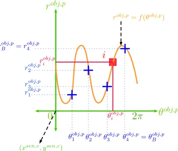
Fig. 3. Visualization of the nonlinear function estimated using the STGP.The figure shows the radial functionrobj,p=f(θobj,p)
(orange) on polar axis (green). The origin corresponds to the IRP i.e. (xsen,c, ysen,c)given in Fig. 2. The measurementi(red square) is
shown for comparison with Fig. 2. The extent state vector (blue plus) consists of radial values (shown on y-axis), which are equidistant points on theθobj,paxis. In this figure, the number of extent states isB= 4.
The function is periodic with period equal to2π. An STGP, trained on coordinates ofiand other measurements reported by the sensor, can model the extent at complete angle domain.
A. Center of a Non-rigid Asymmetric Extended Object
The definition of the CoO depends on the application, for example, for uniformly dense objects the geometric center (centroid) of the object shape is considered as the CoO. For non-uniformly dense objects, it can be defined as the center of gravity or the center of mass. In this paper, objects with uniform density are considered. The CoO of rigid objects is assumed to lie on the same position relative to the object extent at all times. In such cases, a filter with nearly accurate initialization and appropriately modeled dynamics can provide efficient CoO estimates. In contrast, the CoO of a non-rigid asymmetric extended object can shift relative to the object extent. This displacement of the CoO needs to be considered in the CoO kinematics model. In this paper, it is proposed that the estimator does not model the CoO kinematics. Instead, the kinematics of a reference point and the extent states relative to this reference point are modeled. This point lies anywhere inside the object boundary and is called the Internal Reference Point (IRP). The CoO kinematic parameters are determined from the IRP and the extent estimates.
B. Sensor and Object Reference Frames
The extended object tracking problem is modeled in two frames, the sensor (global), and the object (local) frames. The sensor measurements are reported in the sensor (polar or Cartesian) frame. The kinematics of the CoO parameters and the IRP states are modeled in the Cartesian sensor frame whereas the extent states and their kinematics are modeled in the object (polar) frame as shown in Fig. 2. The extent states are radial values of the object extent at an angle from the IRP that is robj,p=f(θobj,p), where(·)obj,p denotes the variable
is in the polar object frame,robj,prepresents the radial extent
and θobj,p represents the angle from the IRP. This is shown in
Fig. 3. The frames and coordinates superscripts are omitted from hereon for brevity.
C. Dynamic Model
The IRP dynamics are modeled using point object motion models [17], [18]. The extent dynamics are designed as separable kernels, which satisfy(C1) to(C4), as given below:
kE(θ, θ′;t, t′) =kE
θ(θ, θ′)ktE(t, t′), (26)
where kE(
·)represents the spatio-temporal covariance kernel,
kE
θ(·)represents the spatial andkEt (·) represents the temporal
covariance kernel. A periodic [20] or Von-Mises [41] covariance kernel can be used to model kE
θ(·). kEt(·) can be modeled
in a number of ways, e.g. squared exponential or Whittle-Mat`ern, which shows the generality of the proposed method. The proposed model is converted to a transfer function form and subsequently to an equivalent state space representation using steps given in Subsection II-B. The dynamics of the IRP and the extent states are assumed independent of each other. The dynamical models are given below:
xIk =fIk(xIk−1) +wIk, wIk∼ N(0,Q I
k), (27)
xEk =FEkxEk−1+wEk, wEk ∼ N(0,QEk), (28)
where (·)I and(·)E denote the vector or matrix corresponds,
[image:6.612.318.496.63.214.2]models [17], [18] can be adopted. The resulting state vector at timek is given below:
xk =
(xI
k)T (xEk)T
T
, (29)
where xk∈Rn
x
represents the overall state vector, xI
k =
(pk)T,(p′
k)T
T
∈RnI denotes the IRP kinematic states, xEk =
(rk)T,(r′k)T
T
∈RnE represents the extent dynamics states, pk andp′k denote, respectively, the position
and its higher order time derivatives, rk and r′k represent,
respectively, the radial extent and its higher order time derivatives. The spatial input of the STGP model is denoted asθ= [θ1, θ2, ..., θB]T which consists ofB keypoints in the
angle domain between 0 and2π, as shown in Fig. 3.
D. Measurement Model
Nk measurements are received from the object boundary at
time k. The coordinates of the sensor measurements can be either polarz˜sen,pk or Cartesianz˜sen,ck . The polar measurement vector is represented asz˜sen,pk =
˜
zsen,p1,k ,· · ·,z˜sen,pNk,kT . Each measurement is modeled as an i.i.d. Gaussian ˜zsen,pi,k ∼ N(µsen,pi,k ,Rsen,pi,k ). The coordinate converted measurement vector in sensor (Cartesian) frame is represented byz˜sen,ck =
˜
zsen,c1,k ,· · ·,z˜sen,cNk,kT
and the corresponding pdf of the ith
measurement at timekis approximated to a correlated Gaussian ˜
zsen,ci,k ∼ N(µsen,ci,k ,Rsen,ci,k ). For the Cartesian sensor measure-ments case, this approximation is not required. After translating
˜
zsen,ck to the IRP and converting the coordinates to polar, the
measurement vectorz˜obj,pk =hz˜obj,p1,k ,· · ·,z˜obj,pNk,kiT is obtained. The corresponding pdf of the ith measurement at time k is
approximated to a Gaussian z˜obj,pi,k ∼ N(µobj,pi,k ,Robj,pi,k ). The relationship among z˜sen,pk ,z˜sen,ck and z˜obj,pk is explained in Fig. 2 and given in Appendix A. The resulting measurement model is given below:
zsen,ck =h(xCk,xkE,z˜obj,pk ,vk), (30)
whereh(·)is a generic measurement function (linear / nonlin-ear) and vk is the measurement noise.
E. Derivation of the Measurement Likelihood Function
The measurement likelihood is derived in this subsection assuming contour measurements. For the surface measurements case, the model derived in this section and a GP convolution particle filter [41] can be used. Alternatively, Kalman filter based approach, given in this paper, can be adopted using a modified spatial covariance kernel as proposed in [1].
[image:7.612.311.565.284.499.2]1) Likelihood function of a single measurement: The like-lihood function is derived for theith measurement. Refer to
Fig. 2 and consider the following vectors:
xobj,ci = ¯xsen,ci −xsen,c, ysen,c= ¯yisen,c−ysen,c, (31)
wherea1−a2 represents the vector difference ofa2 froma1,
(¯xsen,ci ,y¯isen,c)represents the coordinates of the ith
measure-ment and(xsen,c, ysen,c)represents the coordinates of the IRP.
Assuming a noise free environment and using vector algebra the measurement vectors are related to the IRP as given below:
¯
xsen,ci =xsen,c+xobj,ci =xsen,c+ ¯robj,pi cos(¯θobj,pi ), (32)
¯
yisen,c=ysen,c+yobj,ci =ysen,c+ ¯riobj,psin(¯θobj,pi ), (33) zsen,ci =p+µGP
i ζ¯i, (34)
where (¯riobj,p,θ¯obj,pi )represent theithmeasurement predicted
coordinates, zsen,ci represents the ith sensor measurement
vector,p= [¯xsen,ci ,y¯isen,c]T represents the coordinates of the
IRP,µGP i = ¯r
obj,p
i represents the mean of the STGP model at
theithmeasurement angle andζ¯
i= [cos(¯θ obj,p i ),sin(¯θ
obj,p i )]T
represents the ith measurement transformation vector mean. ¯
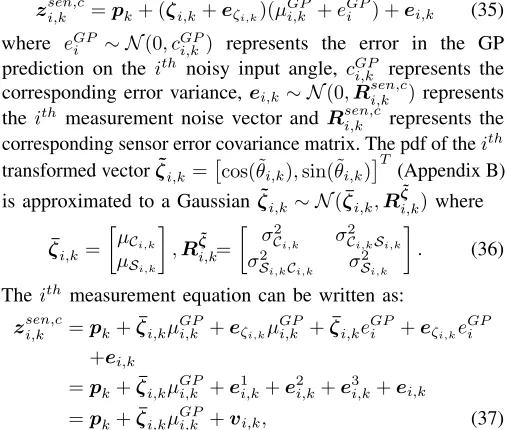
robj,pi is determined using the STGP model prediction and has an associated error represented by the STGP covariance matrix.θ¯obj,pi is calculated using coordinates transform between the sensor and the object frames (Appendix A) and has an associated uncertainty for the noisy measurement case, represented by the pdfp(˜r,θ˜). The sensor and the object frames and coordinates superscripts are omitted from the right hand side of the measurement equation and the time step subscript is added from here on for clarity. The measurement equation with the noise terms is given below:
zsen,ci,k =pk+ (ζ¯i,k+eζi,k)(µGPi,k +eGPi ) +ei,k (35)
where eGP
i ∼ N(0, cGPi,k ) represents the error in the GP
prediction on the ith noisy input angle, cGP
i,k represents the
corresponding error variance,ei,k∼ N(0,Rsen,ci,k )represents
theith measurement noise vector and Rsen,c
i,k represents the
corresponding sensor error covariance matrix. The pdf of theith
transformed vectorζ˜i,k =
cos(˜θi,k),sin(˜θi,k)
T
(Appendix B) is approximated to a Gaussianζ˜i,k∼ N(ζ¯i,k,Rζi,k˜ )where
¯ ζi,k=
µCi,k µSi,k
,Rζi,k˜=
σ2
Ci,k σ
2
Ci,kSi,k σ2Si,kCi,k σ2Si,k
. (36)
Theith measurement equation can be written as:
zsen,ci,k =pk+ζ¯i,kµGPi,k +eζi,kµGPi,k +ζ¯i,keGPi +eζi,keGPi +ei,k
=pk+ζ¯i,kµGPi,k +e1i,k+e2i,k+e3i,k+ei,k
=pk+ζ¯i,kµGPi,k +vi,k, (37)
wherevi,k represents the cumulative measurement error vector
consisting of four error vector componentsei,k,e1i,k,e2i,k and
e3i,k. The components of the noise termvi,k are derived below
e1i,k ∼ N(0,(µGPi,k)2Ri,kζ˜ ) =N(0,RGi,k¯ζ˜), (38)
e2i,k ∼ N(0,ζ¯i,kcGPi,kζ¯Ti,k) =N(0,Rζi,k¯G˜), (39) e3i,k ∼ N(0,Rζi,k˜G˜), (40)
Rζi,k˜G˜ = diag
σ2
Ci,kc GP i,k 2π(σ2
Ci,k+c GP i,k)2
, σ
2
Si,kc GP i,k 2π(σ2
Si,k+c GP i,k )2
, (41)
where RGi,k¯ζ˜,Ri,kζ¯G˜ and Rζi,k˜G˜ represent the noise covariance matrices corresponding to the error termse1
i,k,e2i,k ande3i,k,
respectively, anddiag(·)represents a diagonal matrix. The sum of independent Gaussian random variables is a Gaussian given below:
vi,k∼ N(0,Λi,k),Λi,k=R
¯
Gζ˜ i,k +R
¯
ζG˜ i,k+R
˜
ζG˜ i,k +R
whereΛi,k represents theithmeasurement noise covariance
matrix. The likelihood function is given below:
p(˜zsen,ci,k |xk) =N(Υi,k,Λi,k), (43) Υi,k = ¯zsen,ci,k −(pk+ζ¯i,kµGPi,k). (44) 2) Likelihood Function for Multiple Measurements: In this section, the multiple measurement likelihood is given for Nk
measurements using the single measurement likelihood. The measurement equation is given below:
¯
zsen,ck =H(z˜obj,p
k )xk+vk, (45)
whereH(z˜obj,p
k )represents the measurement function and is
given below:
H(z˜obj,p
k ) =H1(z˜ obj,p k )C1(z˜
obj,p
k )C2, (46)
whereH1,C1 and C2 represent the sub-functions ofH. The
matrix multiplication of C1and C2 with the state vectorxk
gives a matrix consisting of the IRP states and the prediction of the object’s extent at the angles defined by Nk measurements
with respect to the IRP. Subsequent multiplication with H1
performs the coordinate frame conversion of the predicted measurements from polar local to Cartesian local and further to Cartesian global. These matrices and the measurement noise are:
H1(z˜obj,p
k ) =
H2 ζ¯1,k o2 · · · o2 H2 o2 ζ¯2,k · · · o2
..
. ... ... . .. ... H2 o2 o2 · · · ζ¯Nk,k
, (47)
H2=
1 0 o(nI−2) 0 1 o(nI−2)
, (48)
C1(z˜obj,p
k ) =
"
InI OnI×nE
ONk×nI Cθkθ¯ + Σ˜θ
kC ′′ ¯ θkθ
2 #
, (49)
¯
θk=θ¯1,k θ¯2,k · · · θ¯Nk,k T
(50) Σθk˜ = diag(σ2θ1,k˜ , σθ2,k2˜ ,· · ·, σθ2˜
Nk,k), (51)
C2=
InI OnI×nE
OnE×nI C−θθ1
, Cθθ=Σθθ⊗InE B
,(52)
vk∼ N(0,Λk =Ω
¯
Gζ˜
k +Ω
¯
ζG˜
k +Ω
˜
ζG˜ k +Ω˜
zG k ), (53)
ΩGk¯ζ˜= blkdiag
RG1¯,kζ˜ RG2¯,kζ˜ · · · RGNk,k¯ζ˜
, (54)
Ωζk¯G˜= blkdiag
Rζ1¯,kG˜ Rζ2¯,kG˜ · · · RζNk,k¯G˜
, (55)
Ωζk˜G˜= blkdiag
Rζ1˜,kG˜ Rζ2˜,kG˜ · · · RζNk,k˜G˜
, (56)
Ωsen,ck = blkdiag R sen,c
1,k R sen,c
2,k · · · R sen,c Nk,k
, (57)
whereOm×n represents anmbynzero matrix,omrepresents
an m-dimensional zero row vector, om represents an m -dimensional zero column vector, ⊗represents the Kronecker product and blkdiag[·] represents a block diagonal matrix. The measurements are assumed independent which gives the structure ofΣθk˜ ,Ω
¯
Gζ˜ k ,Ω
¯
ζG˜ k ,Ω
˜
ζG˜
k andΩ
sen,c
k as block diagonal.
The GP expression appearing inC1(zobj,p
k )andC2and the GP
covarianceCGPk are derived in Subsection IV-F. The multiple measurements likelihood function is given below:
p(˜zsen,ck |xk) =N(Υk,Λk), (58)
Υk= ¯zsen,ck − [pk]×Nk+ζ¯k⊙
µGPk ⊗
1 1
!
,
where [a]×n represents a column vector with n times
repetition of the vectora,⊙represents element-wise product, ¯
ζk = [ζ¯1,k,· · ·,ζ¯Nk,k]T andµGPk = [µGP1,k,· · ·, µGPNk,k]T.
F. GP Prediction at Noisy Input Locations
The input locationsθ¯k in (50) are corrupted by the sensor
noise. This gives a non-Gaussian posterior, which is approx-imated to a Gaussian. The GP prediction given in (4)–(5) is valid for noise-free inputs. The GP prediction for noisy training input locations and non-noisy predicted locations is derived in [20]. In (45), the GP prediction is required at noisy locations using data of non-noisy input locations. This has been derived in [42], [43] for different covariance kernels. Exact first and second moments of the posterior are derived for linear or Gaussian covariance kernels. For remaining covariance kernels (like the spatial covariance kernel), using a Taylor series expansion, the approximate moments are derived. For a given input with distributionθ˜k ∼ N( ¯θk,Σ˜θk), the predictive mean
and covariance are given below:
µGPk =µ( ˜θk) + 1 2
B
X
i=1
βiT r[C ′′
˜
θkθiΣ˜θk],
CGPk =C(˜θk) +T r
h1
2C
′′(˜θ
k) +µ′(˜θk)µ′(˜θk)T
Σ˜θk
i
,
whereµGP
k andCGPk represent the mean and the covariance
of the GP prediction at the noisy input angle measurements, µ( ˜θk)andC(˜θk)represent the noise-free GP prediction mean
and covariance, respectively, andT r[·] is the trace function. The terms on the right side of the summation in both equations can be seen as the correction of the noise free GP mean and covariance values. These are explained in the following equations:
β=Cθθ−1xEk,µ′(˜θk) =C′¯θkθC−θθ1xEk, (59)
C′′(˜θk) =C′′¯θkθk¯ −Cθkθ′′¯ C−θθ1C′′θ¯θk, (60)
C′′¯θkθ=Σ′′θkθ¯ ⊗ h
1 o¯ nE B−1
i
, (61)
C′′θk¯ ¯θk =Σ′′θk¯ ¯θk⊗ h
1 o¯ nE B−1
i
, (62)
C′¯θkθ=Σ
′
¯
θkθ⊗
h
1 o¯ nE B−1
i
, (63)
whereΣ′·andΣ
′′
· represent the first and second differential of
the corresponding noise free GP covariance matrices.
G. CoO Parameter Estimates
The parameters of the CoO kinematics are the posi-tion and the higher order time derivatives of the posiposi-tion. These parameters are calculated from the estimated shape (polygon) in the sensor frame at each time step. Consider
{(xP1ˆ, y ˆ
P
1),(x ˆ
P
2, y ˆ
P
2),· · ·,(x ˆ
P B, y
ˆ
P
B)}represents the coordinates
of the estimated polygon. The positional [44](xC
k, ykC)and the
velocity( ˙xC
k,y˙kC)parameters are determined as given below:
A= 1 2
B
X
i=1
xC k = 1 6A B X i=1
(xPˆ i +x
ˆ
P i+1)(x
ˆ
P i y
ˆ
P i+1−x
ˆ
P i+1y
ˆ
P
i ), (65)
ykC= 1 6A
B
X
i=1
(yiPˆ+yiPˆ+1)(xPiˆyiPˆ+1−xPiˆ+1yiPˆ), (66)
˙ xCk =x
C k −xCk−1
Ts
, y˙kC=y
C k −yCk−1
Ts
, (67)
whereArepresents the area of the polygon.
H. Real-time Inference
The inference can be done using an STGP batch regression. As most of the EOT applications require real-time processing, the estimation of the state space model and the measurement likelihood derived above is done recursively. A real-time recursive filter equivalent to a full GP regression has also been proposed in [1], [21]. The mathematical equivalence of a full GP regression is a smoother rather than a filter [22]. Given a model of the form (27), (28) and (45) a recursive (nonlinear) Kalman filtering and smoothing solution is developed, to estimate the states at each time step. In high nonlinearity scenarios, advance nonlinear filtering and smoothing methods such as sequential Monte Carlo (SMC), Markov chain Monte Carlo (MCMC) are preferred [39].
The processing time of the smoother increases with time and the computation becomes non-real time as more measurement samples are reported. A fixed lag RTSS is proposed for real-time smoothing. It is further proposed to set the lag of the RTSS equal to as long as the states are correlated in time. In short, the real-time inference is achieved using a fixed lag RTSS with lag value set equal tolt.
V. EXTENDEDOBJECTTRACKING USING
WHITTLE-MATERN` TEMPORALCOVARIANCE
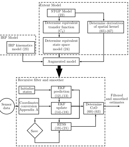
[image:9.612.315.541.54.311.2] [image:9.612.321.551.364.534.2]Section V demonstrates the proposed method using different models. A block diagram of the proposed method is given in Fig. 4.
A. Extent Evolution Model
1) Spatial Covariance Kernel: The periodic spatial covari-ance kernel [20] is illustrated in Fig. 5 and is given below:
kEθ(θ, θ′) =σf2e−
2 sin2 θ−θ′ p
l2
θ +σ2
r, (68)
where σf2, σr2, pand lθ are hyperparameters. σf2 controls the
correlation magnitude, σ2r is the prior radial variance, p is periodicity and lθ controls correlation length-scale. This kernel
is generic and can be used for various real-world extended
objects. Given ϑ= cos
2ε
p
andε= ¯θ−θ′, the derivatives of the covariance kernel are given below:
k′θ(¯θ, θ′) = d dθ¯
kθ(¯θ, θ′)
=− σ2 fe ϑ−1 4l2 θ sin 2ε p
2l2
θp
, (69)
k′′θ(¯θ, θ′) = d dθ¯
k′(¯θ, θ′)
=−σ
2
fe ϑ−1
4l2 θ (4l2
θϑ+ϑ2)−1)
4l4θp2 ,(70)
STGP Model (22)
Determine equivalent transfer function
(C4)
Determine equivalent state space model (24) IRP kinematics model (23) Augmented model Determine derivatives of spatial kernel
(65)-(67) Extent Model IRP Model Initialize states Sensor data Coordinates conversion Appendix A EKF prediction (12),(13) EKF update (14)-(18) RTSS (19)-(21) Save Determine CoO (60)-(63) Recursive filter and smoother
Filtered and smoothed
estimates
Fig. 4. Proposed method. The figure shows the proposed method. The top half (blue) of the figure shows the modeling part whereas the bottom half shows the recursive filtering and smoothing solution. The diamond shape represents a memory storage, required by the RTSS.
l /2 (p) 3 /2 (2p)
r 2 r 2+ f 2
k ( , ,)
Fig. 5. Spatial (Periodic) covariance kernel.
kθ′′(¯θ, θ′) = ∂ ∂θ∂θ¯ ′
h ∂
∂θ∂θ¯ ′
k(¯θ, θ′)i
= σ
2
f l8θ exp
cos(ε)−1.0
lθ2
−cos(2ε)
2 +
cos(4ε)
8 −
3l2θcos(ε)
2 +l
6
θcos(ε)
+3l
2
θcos(3ε)
2 +
7l4θcos(2ε)
2 −
l4θ
2 +
3 8
. (71)
2) Temporal Covariance Kernel: A Whittle-Mat`ern temporal covariance kernel [45], [46] is chosen and is given below:
ktE(t, t′) =σt22
1−ν
Γ(ν)
√2 ν lt τ ν Kν √2 ν lt τ , (72)
whereτ =t′−t,Γ(·)is the gamma function andσ2
t represents
the correlation magnitude andltrepresents the temporal
smoothness of process is determined by the kernel parameter
ν. The corresponding spectral densityS(ωt)is given below:
S(ωt) =σ2t
2π12Γ(ν+1
2)
Γ(ν) λ
2ν(λ2+ω2
t)−(ν+ 1
2), (73)
where ωt represents frequency and λ=
√
2ν
lt . As the
spec-tral density is a function of ω2
t, a stable transfer function G(ιωt) = (λ+ιω)−(p+1) can be obtained after spectral
fac-torization of the given kernel where p=ν−12 and:
qt=
2σ2
tπ 1
2λ(2p+1)Γ(p+ 1) Γ(p+1
2)
, (74)
where qt is the spectral density of the white noise process
driving the temporal evolution of the states.
Remark 1: Choosing the order of the Whittle-Matern
covariance function, ν = 12, yields the Ornstein-Uhlenbeck function [47]. This in turn has the same state-space representa-tion as the model used in GP-EKF [1]. Hence, the GP-EKF can be seen as a special case of the method proposed herein.
3) Extent State Space Model: The system matrix and the noise effect vector of the corresponding state space model for
ν =52 are derived in [23] and given below:
A=
0 1 0
0 0 1
−λ3 −3λ2 −3λ
, L=
0 0 1
. (75)
Using above a multidimensional discrete time state space model for B keypoints is derived and given below:
xEk =FExEk−1+wEk,FE=IB⊗eATs (76)
wEk ∼ N(0,QE(θ,θ′;Ts)), (77)
QE(θ,θ′;Ts) =Cθθ[IB⊗Q˜(Ts)],
˜ Q(Ts) =
Z Ts
0
FE(Ts−τ)LqtLTFE(Ts−τ)Tdτ,(78)
whereFE andQE(θ,θ′;Ts)represent the discrete time state
transition matrix and the process noise covariance matrix for
B keypoints, respectively.
B. IRP Kinematics Model
The IRP kinematics are modeled using a nearly constant velocity (NCV) [17] motion model as given below:
xIk=FIxIk−1+wIk, wIk∼ N(0,Q I)
, (79)
FI = diag( ˜FI,F˜I), QI = diag(qxQ˜ I
, qyQ˜ I
), (80)
˜
FI =
1 Ts
0 1
, Q˜I =
"T3 s
3
T2 s
2
T2 s
2 Ts
#
, (81)
whereqx andqy represent the process noise variances.
C. State Vector
The corresponding state vectors are given below:
xIk=
xk x˙k yk y˙k
T
, (82)
xE k =
r1
k r˙1k r¨1k · · · rkB r˙Bk ¨rkB
T
, (83)
where the location of the IRP is represented by xk, yk and
the velocity of the IRP is represented by x˙k,y˙k. The extent
states consist ofB radial values from the IRP and its first and second time derivatives.
VI. PERFORMANCEVALIDATION
The performance of the proposed method is validated using simulated and real data. The estimates of the proposed method are compared with the GP-EKF estimates [1] over 100Monte Carlo runs for the simulated experiments. The performance evaluation parameters are the positional and velocity root mean square errors (RMSE) of the CoO, the mean shape precision
Pµ and the mean shape recallRµ. These are defined below:
RM SEa=
v u u t
1 K
K
X
j=1
1 NM C
NM C
X
i=1
(ai
j−ˆaij)2, (84)
Rµ=
1 K
K
X
j=1
1 NM C
NM C
X
i=1
Area(Ti j ∩Eji) Area(Ti
j)
, (85)
Pµ=
1 K
K
X
j=1
1 NM C
NM C
X
i=1
Area(Ti j ∩Eji) Area(Ei
j)
, (86)
whereRM SEa represents the RMSE of the parametera,aij
represents the true andˆaij represents the estimated value,Tji
represents the true shape,Ei
j represents the estimated shape,
∩represents the intersection of two star-convex polygons and
Area(p) represents the area of the polygon p. The recall specifies how much of the true shape has been recalled while the precision evaluates the false (not belonging to true object) area. These parameters have been used to evaluate estimators in computer vision for rectangular objects estimation problems [48]. The percentage improvement compared to GP-EKF is also given in the results section. IfRM SEa,RµorPµ
of the GP-EKF is represented by vectorband those of STGP-EKF and STGP-RTSS byc, then the corresponding percentage improvementdand the mean percentage improvementdµ are
given below:
d=b−c
b , dµ = d
K ×100. (87)
A. Simulation Results
The IRP motion model of the simulated object and the estimators is CV with matched process noise variance
qx=qy= 1. Five different shape evolutions are simulated
using two shape models active at different time samples for
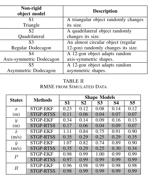
K= 250 time samples. These are the Singer acceleration model [49] and a constant shape model. The shape of the object does not change and the time derivatives of the radial states are zero when the constant shape model is active. The Singer model is active for the time samples in the range k= [(1−50),(80−130),(180−230)]and the constant model is active at all other times. The parameters of the Singer model are maneuver varianceσm2 = 12and maneuver time constantτ = 1s. The shape model and the parameters for simulation are different from the model in filter and smoother. The switching and mismatched shape models further validate the robustness of the proposed method. The different shape evolutions simulated are explained in Table I.
The number of keypoints is B= 24, the sample time is
Ts= 301s, the spatial length-scale islθ= 15◦, the prior radial
variance isσ2
r = 1, the spatial correlation magnitude variance
isσ2
TABLE I NON-RIGID SHAPE MODELS
Non-rigid
object model Description
S1 Triangle
A triangular object randomly changes its size.
S2 Quadrilateral
A quadrilateral object randomly changes its size.
S3 Regular Dodecagon
An almost circular object (regular 12-gon) randomly changes its size. S4
Axis-symmetric Dodecagon
A 12-gon object adapts random axis-symmetric shapes. S5
Asymmetric Dodecagon
A 12-gon object adapts random asymmetric shapes.
TABLE II
RMSEFROMSIMULATEDDATA
Shape Models
States Methods
S1 S2 S3 S4 S5
STGP-EKF 0.23 0.12 0.08 0.14 0.12
x
(m) STGP-RTSS 0.11 0.06 0.04 0.07 0.07
STGP-EKF 0.34 0.14 0.09 0.16 0.13
y
(m) STGP-RTSS 0.17 0.06 0.04 0.09 0.07
STGP-EKF 1.11 0.84 0.75 0.91 0.90
˙ x
(m/s) STGP-RTSS 0.35 0.29 0.25 0.29 0.35
STGP-EKF 1.07 0.82 0.74 0.89 0.90
˙ y
(m/s) STGP-RTSS 0.35 0.29 0.25 0.30 0.34
STGP-EKF 0.98 0.99 1.00 0.99 0.99
P STGP-RTSS 0.97 0.99 0.99 0.99 0.99
STGP-EKF 0.96 0.98 0.99 0.98 0.98
R
STGP-RTSS 0.98 0.99 0.99 0.99 0.99
lt= 2s, the temporal correlation magnitude isσ2t = 1. The
GP-EKF forgetting factor is tuned toα= 0.001. The sensor error standard deviations are σr= 0.25m for range andσθ= 0.25◦
for angle. The number of measurements is Poisson distributed with mean λm= 20. The measurements are located randomly
over the contour of the object using a uniform distribution.
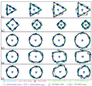
a) Results: The RMSE values and the percentage im-provement from 100Monte Carlo runs for the five scenarios is given in the Tables II and III. The tables show that the performance of the STGP-EKF and STGP-RTSS is improved in all five cases. Fig. 6 shows the snapshots of tracking of a single simulation run of the five scenarios at the selected time steps. It can again be observed that the GP-EKF shape estimates are less accurate as compared to both the STGP-EKF and the STGP-RTSS estimates except for S3 (simplest shape model), where they are comparable.
TABLE III
MEANPERCENTAGEIMPROVEMENT(SIMULATIONS) Shape Models
States Methods
compared S1 S2 S3 S4 S5
STGP-EKF 85.81 86.87 79.85 83.49 85.76
x STGP-RTSS 92.09 93.47 89.66 90.89 91.47
STGP-EKF 77.91 84.74 73.82 83.90 84.17
y
STGP-RTSS 87.55 92.47 87.15 91.50 90.86
STGP-EKF 91.98 90.23 61.90 88.40 87.96
˙
x STGP-RTSS 97.08 96.99 87.53 96.42 95.53
STGP-EKF 91.79 90.43 62.69 88.43 87.85
˙ y
STGP-RTSS 96.60 96.90 87.40 96.50 95.51
STGP-EKF 33.27 14.71 2.01 9.33 8.51
P STGP-RTSS 32.55 14.12 1.70 8.90 8.13
STGP-EKF 18.02 11.21 0.69 7.20 6.59
R
STGP-RTSS 19.62 12.28 1.52 8.20 7.56
B. Effect of the STGP-RTSS Lag Value
The performance of the fixed-lag smoother is evaluated using the shape model S5. The performance is evaluated at different lag values for100 Monte Carlo runs. The smoother lagks is
chosen less than, equal to and more than the true temporal correlation length-scalelt. The results are given in Fig. 7. It can
be observed that the performance of the smoother is degraded forks< lt. However, the smoother performance is comparable
for the cases ks>=lt. Keeping in mind the computational
advantage gained by keeping the lag smaller, as proposed, the
ks=lt is a reasonable trade-off value for the smoother lag.
The peaks in the graphs are observed at time samples when the shape model switches between the Singer and the constant model.
C. Computational Complexity
The computational complexity of the EKF and STGP-RTSS scale asO(N3
kB+Nk2B3)and O(ksB3), respectively.
The empirical results with respect to the three variables B,
Nk andks are shown in Figs. 8, 9 and 10, respectively. The
program was run on MATLAB R2016b on a Windows 10 (64 bit) Desktop computer installed with an Intel(R) Core(TM) i5-6500 CPU @ 3.20GHz (4CPUs) and 8GB RAM. B andks
are the model parameters and can be managed during the design phase. The number of extent states,B, can be decreased in the model according to the available computational resources. At the end of each time-step, the object shape can be constructed as per the requirement using the standard GP prediction (4) and (5). If the object shape is constructed at B0 angles, the increase in computational expense due to this operation is
B0B. Similarly,ks can be reduced according to the available
computational resources. The third variable,Nk, is dependent
on the sensor, the object and other environmental conditions. The processing time can be further reduced through faster code implementation in C++.
D. Real Data
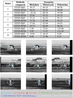
In this section, the proposed method is evaluated on real data presented in [50]. This is a thermal video data of pedestrians and vehicles sampled at 10Hz obtained using a fixed camera in an open environment. Three different video samples are chosen for evaluation which are a motorcycle, a rickshaw and a pedestrian. The rickshaw appears as a regular rigid object, the motorcycle as an irregular rigid object and the pedestrian as an irregular non-rigid object. The ground truth data is not available and is manually generated by marking the object contour (as precisely as possible) in each frame, calculating the CoO location in each frame and the CoO kinematics are determined using the CoO locations of consecutive frames. The video frames are pre-processed using frame differencing and median filtering to generate contour measurements. The following parameters are changed for the real data experiments;
B = 48, lt = 1, σf2 = 30and qx =qy = 50 for the
STGP-EKF / STGP-RTSS andB = 48,σ2
f = 2 andqx=qy = 10
S1
S2
S3
S4
S5
×
measurement True shape bc STGP-EKF shaper
s
STGP-RTSS shape
+
ut GP-EKF shapeb
c
rs ut GP-EKF COO
True COO STGP-EKF COO
STGP-RTSS COO
r
[image:12.612.151.460.51.338.2]s
Fig. 6. Simulated shapes atk= 1,50,150,230. The figure shows snapshots at selected time samples of the five different shape evolutions. The true CoO (red plus) and the shape (red solid line) along with the corresponding estimates are also presented in the figure. It can be observed that except for the S3 the shape estimates of the proposed method are improved as compared to the method [1].
0 20 40 60 80 100
K 0
0.1 0.2
0 20 40 60 80 100
K 0
0.2 0.4
0 20 40 60 80 100
K 0
1 2
0 20 40 60 80 100
K 0
1 2
0 20 40 60 80 100
K 0.98
0.99 1
0 20 40 60 80 100
K 0.98
0.99 1
b
c
[image:12.612.50.300.395.553.2]Nt−58 dl Nt−45 sr Nt Nt+ 60
+
KFig. 7. STGP-RTSS performance at different lag values. The figure shows the comparison of smoother performance at different lag values compared to the true temporal correlationlt. The best performance is given by the smoother
with lagks=Kthat is a full STGP regression. It can be observed that values
less thanltprovide degraded performance while the performance is almost
similar forks>=lt.
Results: The RMSE and the percentage improvement of all three scenarios are given in Tables IV and V. It can be observed that the performance of the proposed approach is comparable to the reference (GP-EKF) method while tracking a regularly shaped rigid object (rickshaw). As observed in the simulated experiments, there is a significant improvement in performance while tracking irregularly shaped objects, especially when the object shape is also changing (pedestrian). The snapshots at three different samples is given in Fig. 11. It can again be observed that the shape estimates (especially the precision) are
20 25 30 35 40 45
0 0.01 0.02 0.03 0.04 0.05 0.06 0.07
Processing time per step(s)
GP-EKF STGP-EKF STGP-EKF-RTSS
Fig. 8. Effect ofBon the processing time. The figure shows a comparison of time taken per time sample by increasingB. The extent state vector of the STGP model is three times the size of the GP-EKF vector. Hence, the STGP-EKF and the STGP-EKF-RTSS require more processing time. AsB increases, the processing time of the STGP-EKF-RTSS rises at a much faster rate compared to the filters due to the RTSS recursion.
significantly improved for non-rigid objects.
VII. CONCLUSIONS
[image:12.612.330.546.395.569.2]5 10 15 20 0.004
0.006 0.008 0.01 0.012 0.014 0.016 0.018 0.02 0.022
Processing time per step(s)
GP-EKF STGP-EKF STGP-EKF-RTSS
Fig. 9. Effect of theNkon the processing time. The figure shows a comparison
of time taken per time sample by increasingNk. The computational cost of
the STGP-EKF increases at a higher rate as compared to the GP-EKF. The STGP-EKF-RTSS computational cost is not dependent on theNkand hence
the plot follows the a similar slope to STGP-EKF with a vertical shift equal to the time required for RTSS recursion.
10 15 20 25 30 35 40
0.005 0.01 0.015 0.02 0.025 0.03 0.035
Processing time per step(s)
[image:13.612.311.565.82.422.2]GP-EKF STGP-EKF STGP-EKF-RTSS
Fig. 10. Effect of thekson the processing time. The figure shows a comparison
of time taken per time sample by increasingks. The computational complexity
of the filter is independent ofkswhile that of RTSS increases exponentially.
TABLE IV RMSEFROMREALDATA
Scenarios
States Methods Rickshaw Motorcycle Pedestrian
STGP-EKF 1.68 1.74 1.63
x
(p) STGP-RTSS 1.11 1.05 1.47
STGP-EKF 2.31 1.50 3.95
y
(p) STGP-RTSS 0.84 1.08 4.00
STGP-EKF 9.13 11.43 6.31
˙ x
(p/s) STGP-RTSS 7.79 7.87 5.51
STGP-EKF 8.35 10.43 14.87
˙ y
(p/s) STGP-RTSS 6.08 8.19 13.41
STGP-EKF 0.99 0.96 0.83
P
STGP-RTSS 0.97 0.93 0.76
STGP-EKF 0.81 0.81 0.84
R
STGP-RTSS 0.89 0.89 0.91
TABLE V
MEANPERCENTAGEIMPROVEMENT(REAL DATA) Scenarios
States Methods
compared Rickshaw Motorcycle Pedestrian
STGP-EKF 30.37 89.18 89.56
x
STGP-RTSS 54.19 93.45 90.58
STGP-EKF -22.16 88.29 43.96
y
STGP-RTSS 55.82 91.53 43.32
STGP-EKF 27.11 82.52 91.11
˙ x
STGP-RTSS 37.78 87.96 92.23
STGP-EKF 37.84 83.04 64.81
˙ y
STGP-RTSS 54.75 86.69 68.26
STGP-EKF 7.58 75.81 135.06
P
STGP-RTSS 5.95 71.67 115.54
STGP-EKF -8.94 16.23 0.20
R
STGP-RTSS 0.60 27.90 9.23
×
measurement True shape STGP-EKF shaper
s
STGP-RTSS shape
+
GP-EKF COO GP-EKF shapeTrue COO STGP-EKF COO
STGP-RTSS COO
b
c
u
t
b
c
rs ut
rs
Fig. 11. Snapshots of three time samples. The figure shows snapshots at selected time samples of the three scenarios, that is rickshaw (top), motorcyclist (middle) and the pedestrian (bottom). The ground truth and the estimates from the STGP-EKF, STGP-RTSS and GP-EKF are also shown. It can be observed that the shape estimates of the STGP based models are improved as compared to the GP-EKF.
the accuracy in position, 95% in velocity and 7% in the shape for the tracking of an asymmetric non-rigid object. The performance improvement to track a non-rigid real object (pedestrian) is up to43%in position, 68%in velocity,10%in the recall and115%in the precision. For complicated nonlinear scenarios, advanced nonlinear filters and smoothers can be derived for the same model using similar steps. Being a general model, it can be applied to solve various real-world problems. The model can also be extended to 3D scenarios.
APPENDIXA
SENSORMEASUREMENTSCOORDINATECONVERSIONS
[image:13.612.66.285.335.502.2]A biased conversion degrades the filter performance [53]. The unbias coordinate conversion has also been proposed namely unbiased converted measurement (UCM) in [54], for polar to Cartesian conversion. In [55], an incompatibility in the UCM derivation was highlighted and removed. The corrected conversion was named modified UCM (MUCM), which was later verified through experiments in [56], [57]. The MUCM conversion is exactly same as proposed in the Appendix of [51]. In this paper, we use the geometric approximate conversion proposed in [51], as the approximation is valid for low sensor noise, which is often the case in EOT / GOT applications.
The sensor measurement noise is modeled i.i.d. Gaussian with variancesσ2
˜
ψi,k andσ
2 ˜
φi,k. The sensor measurement pdf
in polar global frame is z˜sen,pi,k =N(µsen,pi,k ,Rsen,pi,k )
with z˜sen,pi,k = [ ˜ψi,k,φ˜i,k]T, µsen,pi,k = [ ¯ψi,k,φ¯i,k]T
and Rsen,pi,k = diag(σ2 ˜
ψi,k, σ
2 ˜
φi,k). The corresponding
sensor measurement pdf in Cartesian global frame is ˜
zsen,ci,k =N(µsen,ci,k ,Rsen,ci,k ) with z˜sen,ci,k = [˜xi,k,y˜i,k]T,
µsen,ci,k = [¯xi,k,y¯i,k]T, Rsen,ci,k =
σ2 ˜
xi,k σ2˜xi,kyi,k˜
σ2yi,k˜ xi,k˜ σyi,k2˜
,
λb= exp
−φ˜2 i,k
2
¯ ψi,k and
¯
xi,k =λbcos ¯φi,k,y¯i,k=λbsin ¯φi,k, (88)
σxi,k2˜ =
1 2( ¯ψ
2
i,k+σ
2 ˜
ψi,k)[1 + cos(2 ¯φi,k) exp(−2σ
2 ˜
φi,k)]
−exp(σ2φi,k˜ ) ¯ψi,k2 cos2φ¯i,k (89)
σ2yi,k˜ =1 2( ¯ψ
2
i,k+σ
2 ˜
ψi,k)[1−cos(2 ¯φi,k) exp(−2σ
2 ˜
φi,k)]
−exp(σ2φi,k˜ ) ¯ψi,k2 sin2φ¯i,k (90)
σxi,k2˜ yi,k˜ =
1 2( ¯ψ
2
i,k+σ
2 ˜
ψi,k)[sin(2 ¯φi,k) exp(−2σ
2 ˜
φi,k)]
−exp(σ2φi,k˜ ) ¯ψi,k2 cos ¯φi,ksin ¯φi,k (91)
Suppose a [−xk,−yk]T translation is applied to z˜sen,ci,k to
obtainz˜obj,ci,k = [˜xt
i,k,y˜ti,k]T wherex˜i,kt = ¯xi,k−xk+νxi,k˜ =
˘
xi,k +νxi,k˜ , y˜ti,k = ¯yi,k −yk +ν˜yi,k = ˘yi,k +νyi,k˜ and νi,k= [ν˜xi,k, νyi,k˜ ]T =N(0,Rsen,ci,k )represents measurement
noise. The measurement pdf after converting the translated vector to the polar coordinates is approximated to a Gaus-sian z˜obj,pi,k = N(µobj,pi,k ,Robj,pi,k ) with z˜obj,pi,k = [˜ri,k,θ˜i,k]T,
µobj,pi,k = [¯ri,k,θ¯i,k]T and Robj,pi,k =
"
σ2˜ri,k σ2
˜
ri,kθi,k˜ σ2
˜
θi,k˜ri,k σ
2 ˜
θi,k
#
where
σ2ri,k˜ =σ2˜xi,kcos2(¯θi,k) +̺i,k+σyi,k2˜ sin2(¯θi,k) (92)
σ2˜ θi,k =
σxi,k2˜ sin 2(¯
θi,k)−̺i,k+σyi,k2˜ cos2(¯θi,k) ¯
ri,k2 (93)
̺i,k= 2σxi,k˜ yi,k˜ cos(¯θi,k) sin(¯θi,k) (94)
ρri,k˜ θi,k˜ =
(−σ2 ˜
xi,k+σyi,k2˜ )sin(2¯θi,k)+2σxi,k˜ yi,k˜ cos(2¯θi,k) 2σ˜ri,kσθi,k˜ ¯ri,k
(95)
σri,k˜ θi,k˜ =σθi,k˜ ri,k˜ =ρri,k˜ θi,k˜ σ˜ri,kσθi,k˜ , (96)
¯ ri,k=
q
˘ x2
i,k+ ˘yi,k2 , θ¯i,k= tan−1
y˘i,k
˘ xi,k
(97)
The above conversions are approximate and this approximation
is valid in the central and near central regions. If the angular error isσφ˜= 0.5 deg, then the approximation becomes invalid at10σφ˜. Similarly, if
σψ˜
¯
ψ = 0.01, then5%error occurs at5σψ˜.
The sensor errors in the EOT / GOT applications are generally lower and the above approximation remains valid.
APPENDIXB
PROBABILITYDENSITYFUNCTION OFζ˜i,k
Given ζi,k=
cos(˜θi,k),sin(˜θi,k)
T
, the Gaussian approx-imation of the pdf of ζi,k is derived in this Appendix. Suppose, a cosine transformation is applied to a standard nor-mal distribution β∼ N(0, σ2
β). According to Euler’s formula exp(ιβ) = cosβ+ιsinβ and E[exp(ιβ)] = exp
−σ 2 β 2
where E[·] represents the mathematical expectation oper-ator. Also E[eιβ] = E[cosβ + ιsinβ] = E[cosβ] + ιE[sinβ]. As a result, the real and imaginary parts can
be equated as ℜ{E[eιβ]}= exp
−σ 2 β 2
=E[cosβ] and
ℑ{E[eιβ]}= 0 =E[sinβ], respectively, whereℜ{.} andℑ{.}
represent the real and imaginary parts of the variable. Now consider cosine and sine transformations applied to
˜
θi,k∼ N(¯θi,k, σ2θi,k˜ ) with σθi,k˜2 =σβ2, Ci,k= cos(˜θi,k) and
Si,k= sin(˜θi,k). Given that β = ˜θi,k−θ¯i,k, the mean and
variances are approximated as follows:
µCi,k=E[cos(˜θi,k)] =e
−
σ2˜ θi,k
2 cos ¯θ
i,k, (98)
µC2
i,k=E[cos
2(˜θ
i,k)] = 1 2+
1 2e
−2σ2 ˜
θi,kcos 2¯θ
i,k, (99)
σC2i,k=E[cos2θ˜i,k]−(E[˜θi,k])2 = 1
2 + 1 2e
−2σ2 ˜
θi,kcos 2¯θ i,k−e
−σ2 ˜
θi,kcos2θ¯ i,k,
µSi,k=e− σθi,k2˜
2 sin ¯θ
i,k, (100)
σS2i,k= 1 2 −
1 2e
−2σ2 ˜
θi,kcos 2¯θ i,k−e
−σ2 ˜
θi,ksin2θ¯
i,k, (101)
σ2Ci,kSi,k=σ2Si,kCi,k =E[{cos(˜θi,k)−E(cos(˜θi,k))}×
{sin(˜θi,k)−E(sin(˜θi,k))}] = 0, (102)
where µCi,k and µSi,k represent the mean, σ2
Ci,k and σ
2
Si,k
represent the variances and σ2Ci,kSi,k and σS2i,kCi,k represent the covariances. Using above, the pdf can be approximated to a Gaussianζ˜i,k ∼ N(ζ¯i,k,Rζi,k˜ )where:
¯ ζi,k =
µCi,k µSi,k
,Rζi,k˜ =
σ2
Ci,k σ
2
Ci,kSi,k σ2Si,kCi,k σS2i,k
. (103)
The approximation is valid in central and near central regions as explained in the Appendix A.
ACKNOWLEDGMENT