Some aspects about milling : expert system for cutting parameters selection and control designs

Rubio Rodriguez, Luis and De la Sen Parte, Manuel

Some aspects about Milling: Expert System for cutting parameters selection and Control Designs

Original Citation

Rubio Rodriguez, Luis and De la Sen Parte, Manuel (2006) Some aspects about Milling: Expert System for cutting parameters selection and Control Designs. In: Advanced Technologies: Research, Development and Application. ARS publishers, Germany. ISBN 9783866111974

This version is available at http://eprints.hud.ac.uk/16024/

The University Repository is a digital collection of the research output of the University, available on Open Access. Copyright and Moral Rights for the items on this site are retained by the individual author and/or other copyright owners. Users may access full items free of charge; copies of full text items generally can be reproduced, displayed or performed and given to third parties in any format or medium for personal research or study, educational or not-for-profit purposes without prior permission or charge, provided:

• The authors, title and full bibliographic details is credited in any copy;

• A hyperlink and/or URL is included for the original metadata page; and

• The content is not changed in any way.

For more information, including our policy and submission procedure, please contact the Repository Team at: [email protected].

Some aspects about Milling: Expert System for

cutting parameters selection and Control Designs

Rubio, L., De la Sen, M. & Ibeas, A.

are with the IIDP at the UPV/EHU in Spain.

1. Introduction

Milling is a mechanical process which consist of the relative movement between feeding the work-piece and rotating the multitooth cutter, to remove material from the work-piece. Milling is used in industry for the manufacturing of mechanical components. During a operation static and dynamic effects can lead to undesared states, such as stick slip friction and forced and self-excited oscillations (Wiercigroch & Budak 2001). These oscillations, also called chatter oscillation, can culminate in non-smooth work-piece surface, inaccurate dimensions and excessive tool wear (Altintas 2000 , Landers 1997). The regenerative effect is the most widely recognized which causes chatter. Spindle speed selection or modulation and absorbers vibrations are the main solutions to supress chatter without reduce the productivity (Ganguli 2005). But, the difficulties to introduce these techniques and the increasing competence lead to use intelligent techniques to evaluate process parameters, such as, time requeriments, programmed cutting parameters, machine tool selection and/or cuting tools selection (Wong & Hamouda 2003).

2. Milling system description

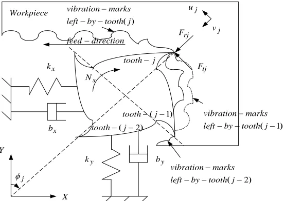
The dynamic milling system is modelled by the interaction between the tool and the work-piece. The milling cutter and the work-piece are usually represented by transfer functions with multiple degrees of freedom, which are obtained from the experimental modal analysis. The model developed here assumes the cutter to have two orthogonal degrees of freedom and the work-piece to be rigid (figure 1).

A. Dynamic model

Then, the dynamic model of the milling cutter has a mode of vibration in each direction, X and Y, while the feed direction of the work-piece is along the X-axis. The milling cutter has n_t teeth, which are equally spaced. Thus, the dynamics of the system is given by the differential equations (Li, H. and Li, X.):

( )

( )

( )

t F

( )

t F y k y c y m t F t F x k x c x m y n j yj y y y x n j xj x x x t t = = ⋅ + ⋅ + ⋅ = = ⋅ + ⋅ + ⋅

∑

∑

− = ⋅ ⋅⋅ − = ⋅ ⋅⋅ 1 0 1 0 (1)

where x and y are the dynamic displacements of the cutter structure into the

X and Y axes, m_i,c_iand k_iare the mass, damping and stiffness of the tool, F_xjand

X Y x k y k x b y b s N j φ j u j v rj F tj F j tooth− ) ( −1

− j tooth

) ( −2

− j tooth ) ( j tooth by left marks vibration − − − ) ( −1

− − − j tooth by left marks vibration ) ( −2

[image:3.595.163.440.122.318.2]

− − − j tooth by left marks vibration Workpiece direction feed−

yj

F are the projections into the two orthogonal axis of the cutting force, F , applied by the jthtooth on the work-piece.

B. Cutting force model

A simple model of the cutting forces will be discussed in this sub-section which expresses the tangential cutting force to be proportional with the instantaneous chip thickness.Despite this simplicity, this model captures the essence of the process. Hence,

( )

t K b h

( )

t

F_t = _t ⋅ ⋅ (2)

where K_t is the specific cutting force parameter, bis the axial depth of cut measured perpendicular to the figure 1 plane, and h

( )

t is the instantaneous chip thickness. In addition, the radial force may also be expressed in terms of the tangential force as,

( )

t K F

( )

t

F_r = _r ⋅ _t (3)

where K_ris a proportional constant. This cutting force model has been widely used by several authors, and was first proposed by Kroenigsberger, A. and Sabberwal, S.

C. Un-deformed cut chip thickness

The most critical variable in (2) is the chip thickness because it changes not only with the geometry of cutting tool and cutting parameters, but also with the uneven surface left by the previous passes of the cutting tool. Hence, after determining the chip thickness for an uncut fresh surface, this thickness must be compared with the undulations left by the cutting tool during subsequent passes at the same position to obtain the instantaneous thickness of the material left to be removed. This process is known as regenerative chatter. The total chip load consist of a static part, h_st, and dynamic components caused by the vibrations of the tool at present and previous tooth periods. This dynamic contribution to the chip-thickness can be modelled through a set of parameters usually known as inner ν _j, and outer ν _j,o, modulations :

(

) ( )

(

hst j o j g j

)

h= + ν _, −ν ⋅ φ (4)

st

h is attribuited to rigid body motion, determined from the feed per tooth s_t by:

j t

st s

The chip thickness is measured in the radial direction, with the coordinate transformation,

j j

j x φ y φ

ν =− ⋅sin − ⋅cos (6) being xand ythe dynamic displacements of the cutter structure at the present period. The dynamic displacements of the cutter at previous tooth periods, νo_jis usually modulated by the value of ν _j−1of previuos tooth

(

j−1

)

.

Then, the regenereative chatter is modelled as (Altintas, Y. 2000),

( )

( )

[

(

)

( ) (

)

( )

]

( )

( ) ( )

( )

[

x t t y t t

]

t T t y t T t x t s t h j j j j j t j φ φ φ φ φ cos sin cos sin sin ⋅ − ⋅ − − − ⋅ − − ⋅ − − + ⋅ = (7) where t is time and T is the tooth period.

D. Stability lobes

The chatter stability lobes make up a spindle speed dependent dividing line between stable and unstable axial depth of cut. It is obtained from the knowledge of the system dynamics. The border line between stable and unstable axial depth of cuts is related to the spindle speed as

( )

2

lim 1

2π _+κ

⋅ Λ − = t t R K n b (8) where T T c c R I ω ω κ cos 1 sin − = Λ Λ

= , being Λ_R,Λ_Ithe real and imaginary parts of the eigen-value of the characteristic equation of the dynamic milling equation, n_tthe number of teeth and K_tthe specific tangential cutting pressure.

The relationship between the chatter frequency, ω_c and the tooth passing period,

T, is given by

π ε

ω_cT = +2k (9)

being kthe integer number of full vibration waves (i.e., lobes) imprinted on the cut arc and εthe phase shift between the inner and outer modulations (present and previous vibration marks). The spindle speed is calculated by finding the tooth pass period T,

T n N

t s = _⋅

60

E. Time domain simulations

The stability charts give broad information about a range of milling operation conditions, indicating the stable and unstable combinations of the axial depth of cut and the spindle speed. To improve the accuracy of the predictions and to gain more insight into the cutting operation, time domain simulation programs have been developed. Simulations are capable of producing information about severity of any resulting vibration, the surface left by the operation, the magnitude of the forces, the frequency of the vibration and so on. The time domain method provides a realistic simulation of the cutting process and chatter instability, since the number of assumptions involved is minimal. Thus, the 4 order Runge-Kutta method is th employed to solve the differential equations (1) in the time domain (Smith & Tlusty 1993, Li & Li 2000).

F. Chatter detection and suppression

An algorithm for the monitorization the detection of chatter and a strategy for the suppression have been extensively researched in the field of the milling process in analytical and experimental ways, for instance see ( Delio et. al. 1992, Landers 1997). In this section, it is intended to give an analytical method to chatter detection. On the other hand, the suppresion of chatter has been widely researched. The main ways are spindle speed selection, spindle speed modulations and vibration absorbers.

1) Chatter detection

The automatically chatter suppression leads firstly to necessity of an algorithm to detect the vibration. Analytically, Li et. al. 2003 proved the effectiveness of the criteria based on the predicted forces. The algorithm visualizes the relative displacements between the tool and the work-piece through a statistical value which measures the oscillations due to the regenerative effect. The non-dimensional coefficient,η, is defined as:

( )

( )

st

dy

F F

max max

=

η (11)

where F_dyis the cutting force predicted using dynamic cutting force model where the regenerative effect of the equation (7) is taken into consideration, and F_stis the resulted cutting force using the static cutting force model and the cutting tool and the work-piece remain rigid. The threshold of instability is selected to be 1.3, then,

3 . 1

≥

2) Chatter suppression

Chatter affects the performance of milling machine, limits productivity of cutting processes, causes poor surface finish, reduces dimensional accuracy, increase the rate of tool wear and reduce the life of milling machine. Conservative cutting

conditions, using the lobes charts, is the most extensive method used in

manufacturing environments to avoid chatter. However, great efforts have been done to increase the productivity without losing efficiency.

a) Spindle speed selection

Other technique which uses the stability charts to suppress chatter is by adjusting the spindle speed to stay within two lobes. In this way, the milling system provides their maximum depth of cut for a given spindle speed increasing the system productivity. The selected lobes are depended on the machine tool requirements such as spindle power or spindle torque.

The main drawbacks are the systems with several coupled modes and the changes in the system parameters due to changes in the work-piece geometry upon cutting. A more detailed explain can be found in Smith & Tlusty 1992.

b) Spindle speed modulation

Michels, V. et al. demonstrated enhancement of the stability in systems with time varying delay by modulating the point-wise delay,T , in equation (7). In the case of milling, modulation of spindle speed is roughly equivalent to modulation of the time delay between successive tooth inserts occupying the same angular position (Sastry et. al. 2001). Then, the spindle speed is varied about a nominal value, typically in a sinusoidal manner:

(

)

(

f t

)

N

N_s = _so 1+α⋅sin 2π _ss (12)

where N_sois the nominal spindle speed, α is the amplitude ratio, f_ss is the signal frequency and t is the time. Although, there are some analytical approach (Jayaram et al. 2000, Sastry et al. 2001, Insperger et al. 2003, and references therein), even successfully experimental cases (Altintas & Chan 1992) to suppress chatter in this way, it has not been obtained a clear method to program the amplitude and frequency of the sinusoidal wave.

c) Vibration absorbers

slightly to the left and the asymptotic stability boundary shifts up (Landers 2005), improving the stability.

Structural damping can be augmented either by passive or off-line and active or on-line means. Smart fluids such as electrorheological (Wang & Fei 1999) or magnetorheological (Segalman & Redmond 1996) fluids or active damping (Dohner et. al. 2004, Ganguli 2005) are examples to suppress chatter actively.

The above introduced methods enhance production and quality of process avoiding the undesired effects caused by the presence of chatter. Nevertheless, these methods suffer from a number of drawbacks which make their application limited or unprofitable. For example, the application of passive or active dampers in the machine requires the machine to be specifically designed. Furthermore, active dampers based on electro/magneto-rheological elements increase the final cost of the machine and causes additional maintenance work. On the other hand, spindle speed modulation leads to complex analytical systems implementation by usual operators hard in everyday work. In conclusion, the field of chatter suppression is still an open research field whose key point is the determination of an adequate set of cutting parameters avoiding chatter while being this set of parameters easy to find and formulate. In the following section, an expert-system based method is developed as a solution to this problem. The expert system provides adequate values for cutting parameters which not only the stability and absence of chatter in the system but also an improved machine behavior taking by into account an optimality criterion. Thus, expert system appears as a feasible method to deal with chatter suppression and efficiency of the milling process. Moreover, the expert system is able to select an adequate tool among a known available set.

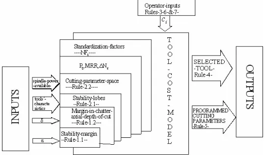
3. Expert mill cutter and cutting parameters selection system

On the other hand, a novel tool cost function is designed to select the operating point. It depends on spindle power consumption, material removing rate (MRR) and on a stability criterion against possible perturbation in the spindle speed variable. Each term of the cost function has a proportional factor to have terms of approximately similar magnitudes. A weight factor which measures the importance of each term is also incorporated.

The proposed cost function is a measure of how the milling process is being carried out at certain operation condittions. The larger the cost function is, the worst operation conditions are. Thus, the cutter and cutting conditions which minimise the designed cost function are selected.

Then, the expert system takes tool characteristics, related tool-work-piece material parameters and milling operation as inputs and outputs the selected tool among the candidates and robust programmed cutting parameters.

A. Milling process determination and preliminary rules

In order to evaluate the system performance, a suitable tool and performance indices are needed. Milling processes, basically, consists of two phases roughing and finishing the surface. The main difference between these operations is to decide the most appropriate performance index for a given tool. The quality and geometric profile of the cutting surface is of paramount importance in milling finishing operation, whereas roughing -milling consists on removing a large amount of material from a blank.

This chapter deals with roughing milling operation. The rate at which the material is removed is called material removing rate (MRR). This parameter measures the productivity of machining processes. In milling operations, MRR is defined as the multiplication between axial and radial depth of cut, spindle speed, and feed. MRR upper limit is given by chatter vibrations and power deliver by the spindle motor. For certain combinations of cutting parameters, such as spindle speed, axial depth of cut and feed, either chatter vibrations are sensed, or the power available by the spindle motor is insufficient. Then, these parameters bound the roughing-milling operation productivity.

For those reasons, the input cutting parameter space is given by the cutting parameters as a first approximation, below the line at the stable stability lobes char while the power consumption is less than the power available by the spindle motor. But, due to uncertainties in the model, the lobes are constructed, not by replacing pure imaginary roots into the characteristic equation, but adding a positive real number to them. Furthermore, to have a robust system, it has been taken into account a confine in a programmed maximum depth of cut.

Then, the following algorithmic methodologies are used, which are called

Rule1: Stability margin setting to ensure that the system plays in a stable region, despite the system model uncertainties.

Rule 1.1: For calculating secure stability lobes char, a small stability margin is selected, i.e, it is supposed that the chatter vibrations happen at δ +i⋅ω_c instead of at i⋅ω_c. The reason is that the stability border line is calculated from a linear approximation. Then, i⋅ω_c is replaced byδ +i⋅ω_c,δ > 0, when the stability border line is calculated. This rule is applied to the equation (13).

Rule 1.2: For improving the robustness of the system, a margin at the final expression for chatter free axial depth of cut has been taken into account, equation (18), i.e, b_lim =α ⋅b_lim,0<α <1. This rule lets a better control capacity in the spindle speed. On the other hand, a better MRR selection is lost because of the above design simplifying process.

Rule2: For searching the allowable input space parameter, the set of spindle speed, Ns, axial depth of cut, b and feed rate, stthe following rules are applied.

Rule2.1: Calculate the boundary points, spindle speed and axial depth of cut pairs, which compose the line between stable and unstable zones, satisfying Rule 1. This rule is obtained by plotting the stability lobes char, which gives the line between stable and unstable zones

Rule2.2: Calculate the admissible input space, Q:=(N_s,b,s_t). The boundaries spindle speed and axial depth of cut, gives the maximum spindle speed and axial depth of cut pairs without chatter vibrations (rule 2.1). The time domain simulation is used to obtain the applied force by the milling machine. As it will be then seen in the next section, the spindle power is force-dependent, which is spindle speed, axial depth of cut and feed rate dependent. Then, for a given spindle motor power available, the admissible input cutting parameter space is obtained.

A. Tool selection

In this section, an approach for tool selection is suggested. For this purpose, a tool cost model function is designed. The designed tool cost model is used to select the appropriate tool between the candidates though the optimization Rules, explained below.

Then, the study requires a given set of candidates milling cutters. Each one is characterized by the following properties:

(

nxi nyi xi yi xi yi ti i i

)

i k k n D

conformed by the pairs

(

ω_nx,ω_ny

)

for each tool, ξ is the set of tools’ damping ratio, conformed by the pairs

(

ξ_x,ξ_y

)

for each tool and tools’ static stiffness is conformed by

(

k_x,k_y

)

for each tool.

B. Tool cost model definition

To carry out the selection of a suitable tool, a novel tool cost function has been conceived. The tool cost model for a single milling process can be calculated using the equation (20).

(

)

s t

s

t MRR N R c c c NF P c NF _MRR c NF _N

P

C , ,∆ ; , ₁, ₂ = ₁⋅ ₁⋅ + ₂⋅ 2 + ₃⋅ 3_∆ (13)

with 1

3

1

=

∑

= i

i

c ,

R

∈

T

, where

∑

( )

= ⋅

= nt

j

j tj

t V f

P

1

φ ,

t s t N n

s b a

MRR= ⋅ ⋅ ⋅ ⋅ , ∆N_stakes its definition given below, andq≡

(

N_s,b,s_t

)

∈Q. Standardizing factors, NF_i, are defined as follow,

1 1 = P_tAv−

NF , where P_tAvis the power available in the spindle motor,

max

2 MRR

NF = , where MRR_maxis the maximum MRR with the chatter vibrations and spindle power restrictions calculated among all the candidate cutters and NF₃ =∆N_s,maxwhere ∆N_s,maxis the maximum measured value of this variable among the candidate cutters.

The tool cost function is designed to minimize a tradeoff amongMRR, power consumption, and a range against possible perturbations in tool rotational motion, dependent and inversely proportional to MRR and a range against possible perturbations and directly to power consumption. The designer keeps the capability of designing the weight of each of those terms according to design requeriments. He also keeps the capability of on-line adjusting such weights. A condition to be fulfilled is the scheme´s stability. For that purpose, all admisible operation points have to belong to the stability region delimited by the lobes which is corrected in the context of a worst case situation, so as to deal with possible uncertain locations of the operation points due to uncertainties in the model like for instance, unmodelled nonlinearities, neglected high-order harmonics and external disturbances.

These parameters have the following definitions: Material or Metal -Removing Rate

(

MRR

)

s t t n N

s b a

MRR= ⋅ ⋅ ⋅ ⋅ , beinga the radial depth of cut, b the axial depth of cut, n_t

parameter, which compares, the efficiency of the milling process. A larger MRR

improves the process productivity.

Cutting power draw from the spindle motor

( )

P_t

The cutting power,P_t, drawn from the spindle motor is found from,

( )

∑

= ⋅

= nt

j

j tj

t V F

P

1

φ (14)

being V =π ⋅D⋅N_s the cutting speed and Ns the spindle speed. The tangential

cutting force is given by:

( )

j t

( )

j

tj K b h

F φ = ⋅ ⋅ φ (15)

where b is the axial depth of cut, Ktis the cutting force coefficient, which are

material dependent and is evaluated from experiments, and h

( )

φ_j is the chip thickness variation, which is feed rate s_t (mm/rev-tooth) dependent.

Spindle speed security change

(

∆N_s

)

An additional term, spindle speed security change, is added to the cost function model to be sure that chatter vibrations are avoided. The spindle speed security change, ∆N_s, measure the nearest spindle speed at which chatter vibrations happen to the supposed spindle speed it will be operated. This fact allows having an error margin due to possible perturbations in this variable.

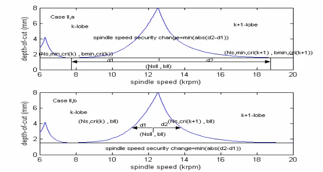
To calculate analytically,∆N_s, the following algorithmic methodologies are carried out. They are divided in two cases:

Case I:k =0, this case corresponds to pairs, spindle speed-axial depth of cut, situated below the first lobe of the stability chars. Then, there is no lobe in the right part of the point. Suppose that

(

N_sI,b_I

)

is the point which ∆N_s has to be calculated:

a) If b_min,cri >b, ∆N_s =abs

(

N_s,min,cri −N_s,I

)

. b) If b_min,cri <b, ∆N_s =abs

(

N_s,cri

( )

b_I −N_sI

)

.

cri

b_min, is the minimum value of the axial depth of cut corresponding to the border line, N_s,min,criis its corresponding spindle speed, N_s,cri

( )

b_I is the left-projection of the point

(

N_sI,b_I

)

into the nearest lobe.

( )

k

N_s,min,cri is the spindle speed corresponding to the axial depth of cut minimum value on the border line, b_min,cri

( )

k , for the k-lobe. Then:

a) If b_min,cri

( )

k >b <b_min,cri

(

k+1

)

( )

(

)

(

(

)

)

(

s cri s s cri s

)

s abs N k N abs N k N

N = − + −

∆ min _,min, , _,min, 1

b) If b_min,cri

( )

k <b>b_min,cri

(

k+1

)

( )

(

)

(

(

)

)

(

scri s scri s

)

s abs N k N abs N k N

N = − + −

∆ min _, , _, 1

where N_s,cri

( )

k is the left-projection of the point

(

N_sII,b_II

)

into the k-lobe, and

(

1

)

, k+

N_scri is the right-projection into the k+1-lobe. The case under consideration is graphically represented in figure 2.

Furthermore, the other possible cases in the ∆N_s calculation are not considered, since they are unstable states cases. On the other hand, the calculated ∆N_s have been done taking into account Rules 1.1 and 1.2. Standardization factors,NF_i, are also added to the cost function to have terms with the same magnitude. Moreover, they make to have a relative term among all the candidates cutters involved. On the other hand, these terms ensure that the cost function will be comparable among the different cutters.

[image:13.595.141.471.308.484.2]

The values are the weights of the cost function terms. They c_i,i=1,2,3 measure the importance of the cost function terms. The below optimization Rule 3 give a pattern to program the parametersc_i.

C. Optimization rules

The above defined tool cost function is used to select the appropriate tool and cutting parameters, through the following optimization rules.

Rule 3: Weight factors selection

The weight factors are intended to be programmed by the machine operator. An extended explanation of their meaning and their adequate selection is given in this section To select suitable values of c_i, i=1,..,3, their meaning has to be perceived. The c₁-value measures the importance of the spindle speed consumption. A larger

1

c parameter is the more important to the spindle power consumption in the cost model function. The c₂measures the machine productivity if the c₂is near to one high productivity is required and if it is near to zero the productivity has no importance. The same reasoning is applied to thec₃, which measures the stability against possible perturbations in the spindle speed variable.

It has to be taken into account that the expert system, ensures that the spindle power consumption is always going to be smaller than the power available in the spindle motor, through Rule 1. Also, that the cutting parameter space has no sensed chatter vibrations through Rule 2.

Then, a possible criterion leading to a process with acceptable productivity, which is the main objective of the milling processes, c₂about 0.75, and the other two constants will add0.25, suitable values are c₁=0.1 andc₂ =0.15.

Rule 4: Tool selection criterion

A simple tool selection criterion for cutter selection has been developed. For a given values of c₁,c₂,c₃, and a given tool characteristics, the cost function value is obtained for all the admissible input cutting parameter space. The minimum value of the cost function is stored. The procedure is repeated for all the available cutters. Comparing the minimum value of the cost function for all available or candidate cutters, the corresponding cutter to the minimum value of the minimum value of the cost function is the selected tool.

The selection criterion is, mathematically, expressed as: Compute,

( )

( )

( )

(

P q ,MRR q , N q ;R ,c1,c2

)

C _{tj j j j} ∆ _{sj j i} (16)

for each R_i∈T,

_

N

i∈ , and

_

Nis the set of candidate tools and

(

sj j tj

)

j N b s

q ≡ , ,

∀ where j∈N _p =

{

1,..,N_p

}

is a discrete sub-space of the cutting parameters space where the cost function (20) is calculated.

( )

( )

( )

(

)

{

, , ; , 1, 2

}

min

arg C P q MRR q N q R c c

ST _{t j j s j i}

N i

∆ =

∈

(17) withST∈T, obtaining the appropriate tool according to the criterion.

Following the rules, the expert system provides an appropriate cutter among the candidates.

Note that the objectives of the expert system are to obtain a tool which has an operating point or adequate cutting parameters where the MRR will be higher than the others available tools, with a prescribed stability robustness and without consumption more power than the available in the spindle motor. Hence, the tool cost model is designed so as to minimize it. Furthermore, the power consumption will be minimum, and the MRR and stability robustness will be maximum, for a given values ofc₁,c₂, andc₃. Thec_i,i=1,2,3, are designed by the machine operator.

Rule 5: Cutting parameter selection

To obtain the cutting parameters a simple criterion, which consist of calculate the cutting parameters which corresponds to the minimum value of the cost function above defined for a certain values of c₁,c₂,c₃. But, here, a new approach thought an auxiliary cost function is going to be applied. In this case, once the tool has been selected, another novel and complete cost function is designed in order to obtain the best cutting parameters. It is composed by the above defined cost functions and other two, which are time and frequency domain responses related. Then, the first new cost function studies the temporal behavior of the input cutting parameters, and the second one its frequency response. The resultant cost function is used to obtain the cutting parameters for the selected tool.

• Temporal response cost model definition

The temporal response cost model is defined as the maximum overshot

( )

M_p and the settling time

( )

t_s dependent function. Those characteristics are typical in the study of the time domain response of a system.

(

)

max , 2

max , 1

2 1 ,

, ,

s s t s

s t t

t j tool

t T Q c c c t _t c M _M

C = ⋅ + ⋅ (18)

where t_s,maxand M_s,maxare the maximum settling time and maximum overshot between the allowable input cutting space parameter, T_toolis the selected tool according with the previous section and

∑

= =

2

1

1

i it

• Frequency response cost model definition

The frequency response cost model is dependent on the relation between the first and the second harmonic frequencies through the function,R_12h, and the relation between the first harmonic frequency and the chatter frequency,R_1ch. That is:

(

)

max 1 12 2 max 12 12 1 2 1 , , , ch h f h h f f f j tool

f T Q c c c R _R c R _R

C = ⋅ + ⋅ (19)

where R_12hmax and R_12chmaxare the maximum of those parameters between the allowable input space cutting parameter, T_toolis the selecting tool according the previous section, and 1

2 1 =

∑

= i if

c ,c_if ≥0.

• Total cost- function model

The total cost function is, then, composed by the defined above three cost functions, the tool cost model, the temporal response cost model and the frequency response cost model.

For this case, the cutting parameters are calculated following the algorithm:

(

)

(

)

(

tool j t t

)

r f

(

tool j f f

)

t r j tool r r r r j tool t resul c c Q T C c c c Q T C c c c c Q T C c c c c Q T C 2 1 3 2 1 2 3 2 1 1 3 2 1 tan , , , , , , , , , , , , , , ⋅ + ⋅ + + ⋅ = (20) where

∑

= = 3 1 1 i ir

c , 0c_ir ≥ , and T_toolis the selected tool.

Compute,C_resultant

(

T_tool,Q_j,c_1t,c_2t,c_3t

)

;∀q_jtool ∈Q_tool, satisfying the rule 22 . . Compute, ⎪⎭ ⎪ ⎬ ⎫ ⎪⎩ ⎪ ⎨ ⎧ = ∀ ( ( , , , , )) min

arg _{tan 1 2 3}

* * r r r j tool t resul q c c c q T C q j

and obtain the input cutting parameters for the selected tool.

Rule6:Process malfunctions: tunning c₁,c₂,c₃values

Nevertheless, in programming the selected tool and cutting parameters, malfunctions of the process may lead to a poor behavior of the process. The most important are tool wear and burr formation (Landers et. al. 2002). These phenomena, which are common in the manufcturing processes, make that the analytical and experimental testes are not always in concordance. If it is happened, the follow algorithmic methodology could be apllied:

where A_chatter is the chatter frequency vibration amplitude, and A_toothpassis the highest amplitude among the tooth passing frequency and its harmonics. So, a more stable state is obtained.

Rule7: Resultant cost function weight factors selection.

To select the values of c_irit has been taken into account the fact that the most important term in C_resultant is C by practical reasons. It is because C_t and C_r are corrected terms. For this reason, it should be taken the c_1r about 0.8, and c_2rand

r

c₃ about 0.1 each one. The time and frequency domains weighting factors,

f f t

t c c c

c₁ , ₂ , ₁ , ₂ are assumed to have the same value or be very similar. Finally, figure 5 shows a scheme of the expert system. The developed expert

system takes the α and δ constants, the tools´ modal parameters such as its natural frequency, damping ratio, tool static stiffness, the number of teeth, the radius of the tool, the helix angle, and the cutting constants for the work material and cutter (tools´ characteristics), the spindle power available and the cost function weight factors, as inputs and outputs the appropriate tool among the candidates and robust programmed cutting parameters.

D. Example

For the validation of this method, the above study has been applied for two practical straight cutters and a full-immersion up-milling operation. The example considers the tools to have the following characteristics, according with the section III.B notation,

(

603,666,3.9,3.5,5.59,5.715,3,30,0

)

1=

R , and

(

900.03,911.65,1.39,1.38,0.879,0.971,2,12.7,0

)

2 =

R .

[image:17.595.163.432.386.544.2]

The natural frequency is measured in hertz, the tool damping is in %, the tool stiffness is in KN ⋅mm−1 and the diameter of the tool is inmm. The work-piece is

a rigid aluminum block whose specific cutting energy is chosen to be

2 2

,

1 =600KN⋅mm−

K and the proportionally factor is taken to bek_r1 =0.3, for the tool one, and k_r2 =0.07 for the other one. Other design expert system parameters are, the stability margin factor, δ =0.05 and the stability margin factor for the axial depth of cut, α =0.95.

The analytical test for mill cutter selection was conducted using spindle speeds with increments of 1000rpm, axial cutting depth started with its minimum value in the stability border line divided by ten, and it is increased in steps of this same size, for a given spindle speed. The operation constraint on the maximum feed per tooth is 550. mm and the step integration is selected to be 050. . The spindle power availability is745.3W .

The resultant tool is that leading to the minimum tool cost function value.

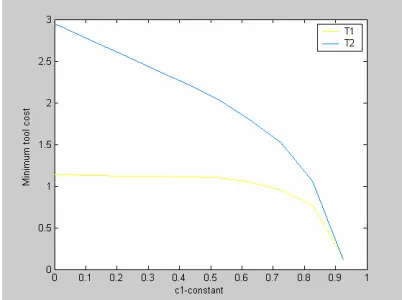
In figure 4, it is shown the values of tool cost function as c₁-parameter varies, thec₃-value has been taken as a constant c₃ =0.075and the c₂ follow the rule

3 1

2 1 c c

c = − − .

This study has been performed to illustrate the influence of the c_iparameters in the tool cost function. It is observed the tool R₁has a better behavior respect to the tool

2

R for all possible value of c₁andc₂, with c₃ =0.075. Analyses with other values of c₁,c₂ and c₃have been carried out and the results are similar, and the tool R₁

has a better behavior.

Then, a more general analysis shows in figure 5, in which the minimum value of the tool cost function for all possible combinations ofc₁,c₂,c₃, with the restriction

1

3 2

1+c +c =

c is displayed.

[image:18.595.202.403.372.522.2]

The analysis has revealed that the first tool has a better behavior than the second one for all combinations of the c_iparameters. Thus the output of the expert system is the first tool.

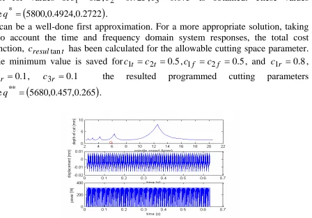
For the cutting parameters selection, two steps have been done. First, the cutting parameter corresponding to the minimum of the tool cost function for the selected tool for values ofc₁ =0.2,c₂ =0.725,c₃ = 0.075 is obtained. These values areq* =

(

5800,0.4924,0.2722

)

.

It can be a well-done first approximation. For a more appropriate solution, taking into account the time and frequency domain system responses, the total cost function, c_resultant has been calculated for the allowable cutting space parameter. The minimum value is saved forc_1t =c_2t =0.5,c_1f =c_2f = 0.5, and c_1r =0.8,

1 . 0

2r =

[image:19.595.187.390.120.271.2]

c , c_3r =0.1 the resulted programmed cutting parameters areq** =

(

5680,0.457,0.265

)

.

[image:19.595.83.531.343.657.2]

Figure 6 shows the situation for the stability lobes of the programmed pointq**, the tool displacement and the power consumption. It is observed that the point is

[image:19.595.173.429.467.653.2]

Fig. 5: Minimum tool cost function versus c₁,c₂,c₃varies

robustly stable and the power consumption is less than the power availability in the spindle motor, while the MRR measure becomes acceptable.

This method can also be applied to any number of selected tools generating in automatic task the best one to be used in the system. Moreover, the method can be used to schedule the relative compliance between the available tools and the used work-pieces materials. On the other hand, the expert system can be used to optimize the manufacturing process, in the sense of planning the adequate sequence of work-pieces to be manufactured for each tool in order to minimize the changes of tools. Finally, apart from being a cheep method, the expert system could be easily used by an inexpert human operator.

According to the established criterion the expert system, once the cutting tool has been selected, provides an operating point in a robust region of the lobes charts, for a given tool, optimizing time and frequency domains reponses and taking into considerartions process malfunctions, such as tool wear and burr formation. On the other hand, it is needed a control strategy to mantain the cutting force below a limit value to prevent fracture of the shank.

4. Milling forces adaptive control under β −FROH discretization

The main objective of control in roughing milling operations is to maintain the cutting force at the desired level, manipulating the feed rate during milling in spite of variation of machining conditions, such as depth of cuts and spindle speed, and then dependent machining parameters, such as time average constants or/and material dependent values. Due to their variations the ideas from adaptive control theory has been widely used. It makes that the term adaptive control of machine tools is applied to systems that range from the simple to the very complex (Koren 1983, Koren 1997, Ulsoy & Koren 1989, Elbestawi et. al. 1990).

In the present section, the adaptive control theory has been applied to prove his efficiency when the milling system changes due to a sudden increase in the cutter immersion, as bench mark, to follow the reference cutting force (Tomizuka 1983, Altintas 2000, Peng 2004).

A. System description

i. Continuous model

1992). Besides, they can be tuned to be over-damped without overshoot, so that they can be approximated to have first order dynamics (Altintas 2000):

( )

_{( )}

( )

1 1 + = = s s f s f s G s c a

s _{τ (21)}

where f_aand f_c are the actual output and command input values of the feed speed in

(

mm s

)

andτ_s is a time constant, which is an average value dependent on the system dynamics, in this study, it is assumed to be 0.1 ms.

The chatter vibration free and resonant free cutting process, which results from equation (1), can be approximated as a first order continuous system (Altintas 2000) :

( )

_{( )}

( )

(

)

1 1 , , + ⋅ = = s n N N ba K s f s F s G c t s ex st c a p p _τ φ φ (22) whereK_c

(

N mm2

)

is the cutting pressure constant, b

( )

mm is the axial depth of cut, and a

(

φ_st,φ_ex,N

)

is the immersion function, which is adimensional and may change between 0 and a proportinal value of the number of teeth, depending on immersion angle and the number of teeth in cut.

The combined transfer function of the system is composed by the feed drive servo and cutting system cascade dynamics,

( )

_{( )}

( )

( )

_{( ) (}

₎

₍

_{) (}

₎₍

₎

1 1 1 1 1 + + = + + = = = s s K s n N ba K s s A s B s f s F s G c m p c t s c m c c c p

c _{τ τ τ τ}

(23) where the process gain is K_p

(

N⋅s mm

)

=K_cab N_tn_s.

The complete system is piecewise constant: admitting sudden changes in the cutting parameters remaining invariant between these changes.

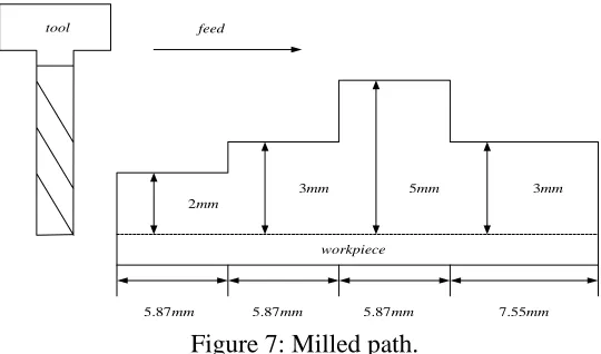
To test the efficiency of the parameter adaptive controller proposes below, it is supossed that the tool have to mill a work-piece with the following geometry (figure 7). An axial depth of cut of 2 mm for a distance of 5.87mm, then 3 mm for 5.87 mm, 5 mm for 5.87 mm, too, and 3 mm for 7.55 mm, as it can be seen in figure 7, respectively in the feed direction with a constant spindle speed of 715 rpm; the work-piece is made of Aluminum 6067 whose specific cutting pressure is assumed to be

2

1200

mm N

ii. Discrete model under β −FROH

A computerized strategy control requires a discrete model. Typically, a zero order hold is used in the manufacturing literature. Here, a fractional order hold of correcting gain β∈

[ ]

−1,1 is used to obtain the discrete transfer function of the continuous system explained above. It provides an extra degree of freedom, β , the gain of the fractional order hold. This extra degree of freedom can used with a broad variety of objectives such as to improve the transient response behavior, to avoid the existence of oscillations in the continuous time output of the system or to improve the stability properties of the zeros of the discretized system. In this way, this work is especially focused on the used of this kind of techniques to improve the transient response of the adaptive system by selecting an adequate value of the fractional order hold. Then, the discrete transfer function is calculated as follow (Bilbao-Guillerna et. al. 2005),

( )

z Z

[

h

( )

s G

( )

s

]

H_β = _β ⋅ _c (24)

where

( )

(

)

s e Ts

e e

s h

sT sT

sT − −

− −

⎟ ⎟ ⎠ ⎞ ⎜

⎜ ⎝

⎛ ₋

+ −

= 1 β β1 1

β is the transfer function of a

FROH

−

β , where zis the argument of theZ −transform, being formally equivalent to the one step ahead operators, q , used in time domain representation of difference equations. This allows us to keep a simple unambiguous notation for the whole section content. The sampling time has been chosen to be the spindle speed, T , as it is usual for this kind of systems (Altintas 2000). Note that, whenβ =1, theFROH hold becomes a first order hold

(

FOH

)

and ifβ =0 the zero order hold

(

ZOH

)

is obtained, as particular cases ofβ ∈

[ ]

−1,1 .

mm

87 .

5 5.87mm 5.87mm 7.55mm mm

2

mm

3 5mm 3mm

tool

[image:22.595.144.414.118.277.2]

workpiece feed

( )

( )

( )

[

( ) ( )

]

(

)

_{( ) ( )}

( )

⎟ ⎟ ⎠ ⎞ ⎜ ⎜ ⎝ ⎛ − ⋅ ⎟ ⎟ ⎠ ⎞ ⎜ ⎜ ⎝ ⎛ − ⋅ = = ⎥⎦ ⎤ ⎢⎣ ⎡ − + − = ⋅ = c m T T c o c o e z e z z z B s s G s h Z Tz z s G s h Z z z z A z z B z H τ τ δ β δ β β β β β β 1 (25)

Furthermore, H_β

( )

z may be calculated just using ZOHin the following way, where

( )

s e s h sT o − −

= 1 is the transfer function of a ZOH and Tis the sampling time, which allows to calculate the β −discrete version of the continuous time plant when only ZOH devices are available. Note that B_β

( )

z depends on β, i.e. a fractional order hold with β ≠0adds a pole at the origin respect to the case β =0 and 0 0 0 1 = ≠ ⎩ ⎨ ⎧ = β β δ_β if if .

iii. Desired response: model reference

The second order system

( )

2 2

2

2 _{n n}

n m s s s G ω ξω ω + +

= is selected to represent the system model reference. This system is characterized by a desired damping ratio of

ξand a natural frequency ofω_n. It is known that small values of ξwould yield short rise time (Kuo 1991). Yet, too small ξ gives a large overshoot and a large settling time. A general accepted range value of ξ for satisfactory performance is between 0.5 and 1, which corresponds to so-called under-damped systems. A damping ratio about ξ =0.75and a rise time, T_r, equal to four spindle periods is selected for practical applications (Altintas et. al. 1990). The natural frequency corresponds toω_n =2.5 T_r rad s(Kuo 1991).

The authors are carrying out a several study of the system output using differents

FROH

−

β holds to obtain the plant and the model reference. Due to extension problems, it will be treated the case which the same β −FROH to hold the plant and the model reference is used. Then, in the present section study,

( )

z Z

[

h

( )

s G

( )

s

]

B. Adaptive model following controller

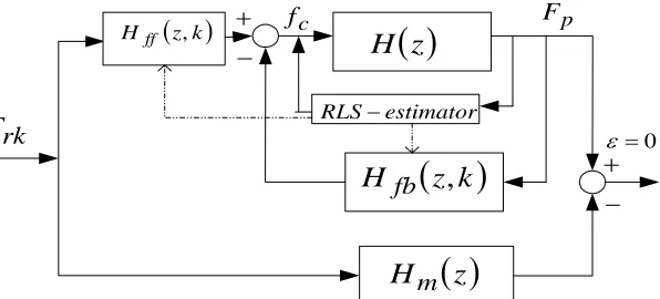
The principle of the model following method is to design a set (pair) of controllers in such a way that the poles of the closed-loop system coincides with a prescribed set of desired poles. These poles are designed according to the required performance of a closed loop system.

Two main steps are involved, the estimation of the parameters of the controlled system, i.e the polynomials A_β

( )

z and B_β

( )

z , which compose

( )

( )

( )

z A

z B z H

β β β = , and the design process of the controller based on these estimated parameters.

When the model plant is not completely known and/or there is measured noise and/or varies with the time an adaptive model following control strategy allows the programmer to place the poles and zeros. But it is necessary to estimate the plant between changes of the cutting parameters. Then, a recursive least square (RLS) algorithm is used to estimate these parameters. In least square estimation unknown parameters of the linear system explained above are calculated using the following RLS with a forgetting factor,λ, at each sampled period k:

( ) (

ˆ 1

) ( ) ( )

[

( ) (

ˆ 1

)

]

ˆ _{k = k − +L k F k −} T _{k k −}

p φ θ

θ θ

( )

(

) ( )

(

( ) (

) ( )

)

1

1

1 + − −

−

= P k k k P k k

k

L φ λ φT φ

( )

(

( ) ( )

)

(

)

λ φ −1 1

−

= I L k k P k

k

P T

(26)

where θˆ

( )

k is the estimated parameter vector at sample k, L

( )

k is the estimation gain, φ

( )

k is the regression or observation vector, P

( )

k is the covariance matrix and

(

0 1

)

, <λ ≤

λ is the forgetting factor. When the forgetting factor takes the value of 1

=

λ the estimation algorithm reduces to the least squares standard algorithm. Alternatively, the smaller the λ value gets, the faster forgets the estimation process oldest data. For simplicity, in the simulations it is usedλ =1.

A pre-compensator and a feedback filter are used to control the plant. The advantages are that the control strategy allows the programmer to place poles and zeros for a unknown plant, with the disadvantage that the control scheme is useless when the system introduces an unstable zero. Thus, the designed control can be applied to inversely stable dicrete systems. The here proposed system introduces a unstable zero of discretization when the β − FROH takes β <−0.6 values. Then, the adaptive control theory has the incovennience that if the unstable zero is unknown it can not be applied.

where

( )

( )

( )

z k R k z S k z H _ff , ,

, = is the feed-forward filter from the reference signal,

( )

( )

_{( )}

k z R k z T k z H _fb , ,

, = is the feedback controller,H

( )

z is the discrete plant, H_m

( )

z is the model reference and F_rk is the reference force.

The desired performance of the closed loop system is represented by the transfer function,

( )

( )

( )

z A z B z H m m

m = , in which the required poles are included in Am

( )

z . In

order to obtain the desired input-output relation, the filters

( )

( )

( )

z k R k z T k z H_fc , ,

, = and

( )

( )

_{( )}

k z R k z S k z H_ff , ,

, = must be adjusted, determining the polynomials T

( )

z,k , R

( )

z,k

and S

( )

z,k .

The polynomial B

( )

z is composed by the stable and monic zeros, B+

( )

z , and the unstables, B−

( )

z , in order to cancel the stable zeros of the system closed loop. The model reference zeros is represented by B_m

( )

z =B_m'

( )

z ⋅B−

( )

z .

( ) ( )

z k T z B

( )

z A

( )

z

T , = = _m' ⋅ _o is time invariant since it only depends on the free selected zeros of the reference model which is composed of constant coeficients andA_o

( )

z is a constant polinomial which is included to ensure good tracking and causality in the design, R

( )

z,k = B+

( ) ( )

z ⋅R' z,k , which is monic.

( ) ( )

z R z k

T , , and S

( )

z,k are the unique solutions of degrees,

( )

2deg

( )

deg

( )

deg

( )

1 deg A_o ≥ A − A_m − B+ −

( )

R deg

( )

A_o deg

( )

A_m deg

( )

A

deg = + −

( )

z H

( )

z k

H _fb ,

( )

z

H_m

+ε =0

rk F − + − c

f Fp

( )z k H_ff ,

estimator

[image:25.595.154.452.115.250.2]

RLS−

( )

deg

( )

1 deg S = A −

( )

_{T =}

( )

_{A +}

( )

_{B −}

( )

_B− m

o deg deg

deg deg

(27)

of the Diophantine equation of polynomials:

( ) ( )

z k R z k B

( ) ( )

z k S z k A

( )

z A

( )

z

Aˆ , ⋅ ' , + ˆ− , ⋅ , = _m ⋅ _o (28)

This leads to design the controller:

( ) ( ) ( )

z k f k T z k F

( ) ( )

k S z k F

( )

k

R , ⋅ _c = , ⋅ _r − , ⋅ _p (29)

The adaptive model following control will be designed for different cases of the transfer function and reference model obtained from β − FROH. In the case of sampling with β =0, a discrete second order plant is obtained,

( )

2 1 2 1 0 a z a z b z b z H o + + + = = β (30)

and a second order model is obatined as a reference,

( )

m m m om m a z a z b z b z H 2 1 2 1 0 , + + + = = β (31)

and if β ≠0, third order models result,

( )

z a z a z b z b z b z H o 2 2 1 3 2 1 2 0 + + + + = ≠ β (32) and

( )

z a z a z b z b z b z H m m m m om m 2 2 1 3 2 1 2 0 , + + + + = ≠ β (33) Then, the parameter vector is θˆ=

[

aˆ₁aˆ₂bˆ_obˆ₁

]

ifβ =0, and θˆ=

[

aˆ₁aˆ₂bˆ_obˆ₁bˆ₂

]

ifβ ≠0. Its initial values are set to arbitrary value ofθ_i

( )

0 =0.2,∀i, where i is the number of estimated parameters for each case.

The regressor vector is namelyφ

( )

k . The covariance matrix P

( )

k is a square matrix whose dimension is the number of the parameters to be estimate, and it is initialized as diagonal with large equal eigen-values

P

( )

0

=

10

5.The covariance matrix is reset to its inititial value each time that the estimation error becomes greater than 5% of the reference force (Altintas et. al. 1990) or by monitoring the trace of the covariance matrix (Altintas 2000).

plotted for the cases of β =−0.3,β =0,β =0.3,β =1, respectively. The figures show the model reference and the plant output signal versus sample time, the tracking error signal, e=

(

F_p −F_pm

)

, the controller response and the time domain system response. The figures present the resultant force keeping at the reference force, which is set to 1.2KN . The system registers large overshots in the transient responses, depending on the β-value, and when the axial depth of cut change abruptly.

[image:27.595.199.399.245.391.2]

The transient responses are relied on the initial values of the parameter vector. If those values are near to real values of the plant, the transient response of the milling system will be smooth and feasible. In contrast, if the initial value of the parameter vector has been selected in arbitrary manner the transient is normally oscillated with great maximum overshot and large setting time, leading to damage or even, break the tool (Altintas 1992 and Altintas et. al. 1988).

Figure 9: Discrete and continuos responses, tracking error, and programmed control law using a β=−0.3- FROH, with θ_i( )0 =0.2.

[image:27.595.202.403.447.595.2]

An accurate transfer function representation of the machining process help the controller designer to have a succesfull implemetation, in the sense that the system transient behaviour is smooth and feasible.

Nevertheless, in spite of being quite robust and stable, the adaptive algorithm encountered large output overshots during dangerous step changes of the axial depth of cut. It is because of the intrinsic structure of the closed-loop output. For this reason, if the reference force is selected near to the tool breakage limit, the large overshot lead to break the tool. To avoid this fact, in Spence & Altintas 1998 is proposed to use a CAD assisted force which is introduced when the axial depth of cut changes to minimize the problem. The only thing they need to know a priori information about the work-piece geometry changes to design a successful adaptive control.

[image:28.595.198.395.171.315.2]

The β −FROH provides a extra degree of freedom. Selecting appropiately the β -value, better transient response behavior will be achieved. Also, less overshots

Figure 11: Discrete and continuos responses, tracking error, and programmed control law using a β =0.3- FROH, with θ_i( )0 =0.2.

[image:28.595.198.397.377.525.2]

betweeen dangerous changes in the axial depth of cut could be obtained. Then, this parameter can be tuned to damp large overshots, such transient responses as between changes in the axial depth of cut. To analyze and compare system responses under differents β −FROH discretizations, a cost function is defined:

(

)

( )

( )

( )

( )

( )

F

( )

dt F

T jT F

jT F dt

t F t F T

Jc

p

p

T

m p p

N T

j

m p p

T

m p p

∫

∑

∫

− ≅

≅ ⋅ −

≅ −

=

=

0

,

0 1

0 ,

0 0

,

0

,

τ τ

β

β

β β

(34)

where F_pis the continuous time domain response, m

p

F _β

, is the discrete response

with a linear interpolation, T is the sampled time, T_ois the discretized time of the computer, T_pis the tested time and N_pis the samples number of the T_operiod over

p

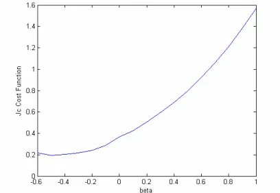
T .The cost function calculates an approximation of the area between the time domain response and the linear interpolation of the discrete response. The smaller the area is the better output response will be respect to system overshoots.

The figure 13 shows the value of the cost function, J_c, for the range of β where the sytem has stable zeros. It can be seen for a β about −0.3, the value of the cost function is minimum and the transient behavior has less overshoot. This fact can be checked in figures from 9 to 12.

Note that the programmed feed rates in case of using a β − FROH or using a

[image:29.595.190.394.419.560.2]

ZOH for discretizasing the milling system are not the same, see figures 9 and 10. Forced feed rates can also be lead to tool failure or breakage (Altintas 1992).