A model based circular binary segmentation algorithm for the analysis of array CGH data

R E S E A R C H A R T I C L E

Open Access

A model-based circular binary segmentation

algorithm for the analysis of array CGH data

Fang-Han Hsu

, Hung-I H Chen

, Mong-Hsun Tsai

, Liang-Chuan Lai

, Chi-Cheng Huang

, Shih-Hsin Tu

,

Eric Y Chuang

and Yidong Chen

Abstract

Background:Circular Binary Segmentation (CBS) is a permutation-based algorithm for array Comparative Genomic Hybridization (aCGH) data analysis. CBS accurately segments data by detecting change-points using a maximal-t test; but extensive computational burden is involved for evaluating the significance of change-points using permutations. A recent implementation utilizing a hybrid method and early stopping rules (hybrid CBS) to improve the performance in speed was subsequently proposed. However, a time analysis revealed that a major portion of computation time of the hybrid CBS was still spent on permutation. In addition, what the hybrid method provides is an approximation of the significance upper bound or lower bound, not an approximation of the significance of change-points itself.

Results:We developed a novel model-based algorithm, extreme-value based CBS (eCBS), which limits

permutations and provides robust results without loss of accuracy. Thousands of aCGH data under null hypothesis were simulated in advance based on a variety of non-normal assumptions, and the corresponding maximal-t distribution was modeled by the Generalized Extreme Value (GEV) distribution. The modeling results, which associate characteristics of aCGH data to the GEV parameters, constitute lookup tables (eXtreme model). Using the eXtreme model, the significance of change-points could be evaluated in a constant time complexity through a table lookup process.

Conclusions:A novel algorithm, eCBS, was developed in this study. The current implementation of eCBS consistently outperforms the hybrid CBS 4× to 20× in computation time without loss of accuracy. Source codes, supplementary materials, supplementary figures, and supplementary tables can be found at http://ntumaps.cgm. ntu.edu.tw/eCBSsupplementary.

Background

Copy number alterations (CNAs) are genomic disorders that closely correlate with many human diseases [1]. For instance, 17q23 was found to be a common region of amplification associated with breast cancers with poor prognosis [2], and copy number losses at 13q and gains at 1q and 5p were frequently observed in a prostate can-cer study [3]. While some CNAs are well studied, most CNAs and their relation to genetic disorders remain lar-gely unknown. Identifying regions of DNA copy number

gains or losses is thus a critical step for studying the pathogenesis of cancer and many other diseases.

Array comparative genomic hybridization (aCGH) is a high throughput and high-resolution technique for mea-suring CNAs [4,5], and the main purpose of aCGH data segmentation is to detect CNAs precisely and efficiently by utilizing neighboring probes’characteristics. Many algorithms have been proposed for this purpose, such as the Clustering Method Along Chromosomes (CLAC) [6], Hidden Markov Model methods [7,8], and Bayesian segmentation approaches [9,10]. Among these algo-rithms, Circular Binary Segmentation (CBS) [11] has the best operational characteristics in terms of its sensitivity and false discovery rate (FDR) for change-point detec-tion [12,13].

* Correspondence: [email protected]; [email protected] 1

Graduate Institute of Biomedical Electronics and Bioinformatics, Department of Electrical Engineering, National Taiwan University, Taipei 106, Taiwan 2

Greehey Children’s Cancer Research Institute, The University of Texas Health Science Center at San Antonio, San Antonio, TX 78229, USA

Full list of author information is available at the end of the article

CBS performs consistently [13] and has been widely used by researchers [14,15], but the major weakness of heavy computational cost prohibits CBS for high-density aCGH microarrays with millions of probes. The original CBS relies fully on a permutation-based maximal-ttest to detect change-points. Through a recursive cut and test process, reliable results can be derived but require extensive computational burden. Realizing the defi-ciency, a hybrid version of CBS that mixes the permuta-tions and a mathematical approximation was recently proposed [16]. Along with additional early stopping rules for approximating the significance of change-points, the hybrid CBS can detect change-points in a linear time and provides a substantial gain in speed.

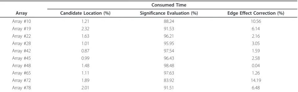
However, further improvements in CBS are still urgently needed. First, the computation time of the hybrid CBS needs to be improved because of the grow-ing density of commercial microarrays. A time con-sumption investigation of the hybrid CBS revealed that the majority of the computation time, about 94% of total time, was spent on significance evaluation, with the bulk of the time being consumed by permutations (shown in Table 1). This finding indicates that limiting permutations may be necessary. Without the improve-ment, for example, it might take days to segment 500 samples generated by the most recently completed ovar-ian cancer study by the Cancer Genome Atlas (TCGA) research network [17]. Second, what the mathematical approximation in the hybrid method provides is an approximation of significance upper bound or lower bound, not an approximation of the significance of change-points itself. As indicated in [16], using an sig-nificance upper bound to reject the null hypothesis may result in fewer change-points.

In this study, we proposed a model-based version of CBS, termed extreme-value based CBS (eCBS). Instead of evaluating an significance upper bound or a lower

bound, eCBS approximates the significance of change-points using a Generalized Extreme Value (GEV) distri-bution model (eXtreme model). The eXtreme model consists of a set of lookup tables built in advance through simulation. Considering a variety of non-normal aCGH data, we simulated thousands of data without change-points using the Pearson system. The corre-sponding maximal-tdistribution was then modeled by the GEV distribution, and the modeling results in the form of the GEV parameters constituted the eXtreme model. Using the eXtreme model, the significance of change-points can be approximated through a table lookup process in a constant time complexity. As a result, permutations are limited and computation time can be significantly reduced. The performance of seg-mentation in speed and segseg-mentation results using both the hybrid CBS and eCBS were compared via simulation and real data analysis.

Methods

Algorithm - Finding Change-Points

Similar to CBS, the newly proposed algorithm, eCBS, detects change-points relying on a sequence of maxi-mal-ttests. Before getting into the details of the maxi-mal-ttest, we first introduce the maximal-tstatistic as follows. Let r1,..., rNbe log2 ratios of signal intensities indexed byNordered genomic markers. LetSi =r1+ ... + ri, 1 ≤ i ≤ N, be the partial sums, and let

Sij=Sj−Si=j_l=i+1rl. StatisticsTijare given by [11]

Tij=

Sij

k −

SN−Sij

N−k

/

s

1

k +

1

N−k

, (1)

where 1 ≤i < j≤N,srefers to the standard deviation ofr1,..., rN, andk=j - i. Among all values ofTijderived from all possible permutes of i and j under

Table 1 The percentage of time consumed on each step of segmentation using the hybrid CBS

Consumed Time

Array Candidate Location (%) Significance Evaluation (%) Edge Effect Correction (%)

Array #10 1.21 88.24 10.56

Array #19 2.32 91.53 6.14

Array #22 1.63 96.21 2.16

Array #28 1.01 95.95 3.05

Array #42 0.87 97.54 1.59

Array #45 0.99 96.43 2.58

Array #48 1.48 98.48 0.04

Array #65 1.11 97.63 1.26

Array #72 1.89 83.92 14.19

Array #78 2.01 91.51 6.48

consideration, the maximal statistic,Tmax, is referred to as the maximal-tstatistic, and the corresponding loca-tions, ic andjc, are termed candidate change-points, which are given by

ic,jc = arg max 1≤i<j≤N

|Tij|, 1≤ic<jc≤N.

Based on the maximal-tstatistic, a maximal-ttest with two hypotheses (H0: there is no change-point,H1: there are change-points locating at ic and jc) is formulated. We reject the null hypothesis H0 and declare locations ic andjcas change-points if Tmax exceeds a significance threshold.

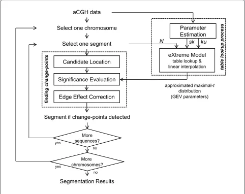
For a chromosome under consideration, similar to CBS, eCBS detects the regions with equal DNA copy numbers by recursively invoking a change-point func-tion, named “finding change-points“, in which two ends of a sequential data are first connected and then ternary splits are determined using the maximal-t test. The function of finding change-points contains three steps: 1) apply maximal-tstatistic to locate candidate change-points ic and jc; 2) determine whether the candidate change-points are significant or not; and 3) if significant change-points occur, a t-test is applied to remove errors near the edges. We refer to these three steps as candi-date location, significance evaluation, and edge effect correction.

The implementation of the process for finding change-points in eCBS is basically the same as CBS except the method for significance evaluation. More precisely, in the original CBS, maximal-tdistribution (distribution of the maximal-tstatistics under null hypothesis) and the significance of change-points are evaluated using permu-tations; in the hybrid CBS, the significance of change-points is approximated using a mixed procedure, consti-tuted of permutations, a mathematical approximation, and early stopping rules. In this study, eCBS approxi-mates the significance of change-points using the eXtreme model through a table lookup process. Indexed by the measures of skewness and kurtosis estimated from the array and the number of probes in the sequen-tial data under consideration, the eXtreme model pro-vides an approximation of maximal-tdistribution in the form of GEV parameters. We will introduce the GEV distribution and the GEV parameters later in the next subsection. We herein demonstrate the implementation of the function - finding change-points - in eCBS as Algorithm 1. Please note that the input variables, gev-Params, represent the approximated maximal-t distribu-tion provided by the eXtreme model. Addidistribu-tionally, gevcdf(Tmax, gevParams) is a function returning the cumulative distribution function of GEV distribution

with parametersgevParams at the valueTmax. See Fig-ure 1 for the overall concept.

Algorithm 1- finding change-points

change points = finding change-points (data, gevParams)

Input: data: aCGH data to be segmented, 1 ×N vec-tor

gevParams: GEV parameters,g,s,μ.

Output:change-points: a list of change-points

Step:

1. Compute statistics, Tij, for all possible locations i andjby Eq.(1);

2. Find candidate change-pointsic andjcwith maximal statistic,Tmax;

3. Evaluate the significance of change-points,p-value, using

p-value = 1-gevcdf(Tmax, gevParams);

4. Edge effect correction;

5. If change-points are detected, list change-points into change-points; also, cut and define new subsegments.

The Table Lookup Process

Accurate approximations of maximal-t distribution using the eXtreme model depend on robust estimators of skewness and kurtosis; incorrect estimates of skew-ness and kurtosis from aCGH data render the table lookup process incapable of finding correct values. Since the estimation of skewness and kurtosis could be biased due to extremely large values [18], a pre-segmentation process - scanning obvious change-points quickly before segmentation - is selected (see Additional File 1: Supple-mentary Materials). The pre-segmentation process (see Algorithm 2) is quite similar to formal segmentation, but with lower resolution and no edge effect correction. After subtracting the changes of mean values from copy number amplifications or deletions, skewness and kurto-sis can be estimated without bias due to CNAs. Since no permutations are involved, the pre-segmentation pro-cess is done in a short time.

Algorithm 2- parameter estimation [sk, ku] = parameter_estimation(data)

Input: data: aCGH data to be segmented, 1 × N vector

Output:sk, ku: estimates of skewness and kurtosis.

Step:

2. Discard small segments;

3. Subtract all segments’mean values;

4. Derive measures of skewness and kurtosis after removing segments’mean values.

The table lookup process for deriving approximations of maximal-tdistribution can be done by sending three indexes, namely, estimates of skewness and kurtosis and the number of probes under consideration, to the eXtreme model. If these indexes do not fall exactly on the table grid, linear interpolation is applied to accom-plish the approximation. We apply linear interpolation because the GEV parameters change smoothly with increasing or decreasing values of skewness, kurtosis, and number of probes (shown later). Through the table lookup process, the eXtreme model can provide accu-rate approximations of maximal-tdistribution when the number of probes in the sequential data under

consideration is not too small (described later). We empirically set the default minimum as 100 probes; when number of probes is less than the minimum, the mixed procedure applied in the hybrid CBS kicks in. Additional improvement in computation time may be achieved using a smaller minimum at the expense of accuracy.

Simulating aCGH Data Using the Pearson System

The basic idea to create the eXtreme model, which associates characteristics of aCGH data with maximal-t distribution, was to simulate a large number of aCGH data and then model the distribution of maximal-t sta-tistics under null hypothesis using the GEV distribution. While a fundamental assumption of aCGH data is Gaus-sian normality, practical microarray data can be non-normally distributed [19]. Additionally, as we observed

Candidate Location

Segmentation Results

eXtreme Model

sk

Edge Effect Correction

N

More sequences? yes

no

Select one segment

Significance Evaluation

aCGH data

Select one chromosome

Segment if change-points detected

More chromosomes? yes

no

Parameter

Estimation

ku

approximated maximal-t

distribution (GEV parameters)

finding change

-point

s

table lookup process

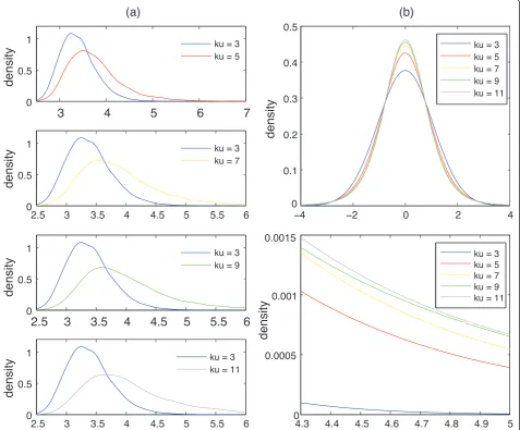
in Figure 2, maximal-tdistribution is quite sensitive to outliers and heavy tails of aCGH data.

Thus, in order to provide accurate modeling results for most aCGH data, we need to consider non-normal properties, namely, the skewness and kurtosis, when generating synthetic datasets.

The Pearson system [20] provides a way to construct probability distributions in which skewness and kurtosis can be adjusted. Without knowing the probability distri-butions from which aCGH data arose, we hypothesized that, by providing up to 4thmoments (mean, variance, skewness and kurtosis), the Pearson system is sufficient to simulate a wide range of aCGH data under null

condition (no change-points). This hypothesis was clearly hold under our simulated condition by the Kol-mogorov-Smirnov Test (KS-test) (see Additional File 1: Supplementary Materials for details of the testing results). Including a set of probability density functions (PDFs), the Pearson system is the solution to the differ-ential equation,

p(x) p(x) =

x−a b2x2+b1x+b0

, (2)

where p(x) is a density function anda, b0,b1, and b2 are parameters of the distribution. Correspondences

3

4

5

6

7

0 0.5 1

(a)

2.5 3 3.5 4 4.5 5 5.5 6

0 0.5 1

2.5

3

3.5

4

4.5

5

5.5

6

0 0.5 1

2.5 3 3.5 4 4.5 5 5.5 6

0 0.5 1

density

−4 −2 0 2 4

0 0.1 0.2 0.3 0.4 0.5

(b)

4.3 4.4 4.5 4.6 4.7 4.8 4.9 5

0 0.0005

0.001 0.0015

ku = 3 ku = 5 ku = 7 ku = 9 ku = 11

ku = 3 ku = 5 ku = 7 ku = 9 ku = 11 ku = 3

ku = 5

ku = 3 ku = 7

ku = 3 ku = 9

ku = 3 ku = 11

density

density

density

density

density

Figure 2Tail effect on maximal-tdistribution. (a) The kernel smoothing density of the maximal-tstatistics derived from 10,000 datasets drawn from the Pearson system (Eq.(2)) with skewness = 0 and various kurtosis. Each dataset contained 250 random numbers. (b) The

between the distribution parameters and the central moments (θ1,θ2,θ3,θ4) [21] are denoted as

b0=−

θ2

4β2−3β12

/A,

b1=−

θ2β1(β2+ 3)

/A,

b2=−

2β2−3β12−6 /A,

where _β1=θ3/

θ3

2 denotes the skewness, and

β2=θ4/θ22 denotes the kurtosis, and

A= 10β2−12β12−18.

A MATLAB function,pearsrnd(), was applied to gener-ate data with different parameters. Again, since these data were generated under null hypothesis, they contain no change-points. Therefore, the maximal-t statistics generated from these data satisfy the null hypothesis. To be specific, we generated tables of data for,

1. The number of probes,N, which varies from 10 to 10,000 with intervals of 10, 100, and 1000 for the number of probes within 100, 1000 and 10000, respectively;

2. Skewness,sk, selected from -1 to 1 with an inter-val of 0.1; and

3. Kurtosis, ku, selected from 2.6 to 5.6 with an interval of 0.2.

Please note that skewness is 0, and kurtosis is 3 for a normal distribution. The ranges and intervals of the simulation parameters were carefully chosen based on typical estimates of skewness and kurtosis from real aCGH data (see Additional File 1: Supplementary Figure. One can always refine the table resolution when improved computation resources are accessible. Note that the mean and standard deviation of the simulated data were irrelevant to GEV modeling due to the nor-malization process in Eq.(1), we thus set the mean and standard deviation for simulating aCGH data to be 0 and 1, respectively.

Modeling Maximal-tDistribution Using the GEV Distribution

After simulating aCGH datasets and the subsequent maximal-tstatistics, we modeled maximal-tdistribution by the GEV distribution with parameters (described later), g, s, and μ, using a maximal likelihood method [22]. Please note that the GEV parameters were derived from the maximal-t statistics, not directly from the simulated datasets. The modeling process was done using a MATLAB function (statistical toolbox), gevfit(), a maximum likelihood estimator of the GEV parameters. As a result, tables of modeling information (one table

for each GEV parameter), indexed by skewness, kurtosis and the number of probes, were generated and saved in the eXtreme model on which eCBS was based.

We briefly go through the GEV distribution and the GEV parameters as follows. For a sequential indepen-dent and iindepen-dentically distributed (i.i.d.) random variables, t1,..., tn, the Fisher-Tippet theorem states that after proper normalization, the maximum of these random variables, tmax = max (t1,..., tn), converges in distribution to one of three possible distributions: the Gumbel distri-bution, the Fréchet distridistri-bution, or the Weibull distribu-tion. The three distributions listed above are unified under the Generalized Extreme Value (GEV) tion [23,24]. The density function of the GEV distribu-tion with parameters (μ,s,g) is given by

f(tmax) = ⎧ ⎨ ⎩σ

−1_w−_γ1−1_e−w− 1 γ

, w>0, forγ = 0

σ−1_e−z_e−e−z

,∀t, forγ = 0

,

where w = (1 + gz), z = (tmax - μ)/s, g is the shape parameter,sis the scale parameter (s>0), and μis the location parameter.

In our setting, the statisticsTijderived from the quoti-ent in Eq.(1), instead of being a seququoti-entiali.i.d. random variables, form a random field spatially correlated in the i -jplane. However, it is not difficult to show that the covariance between any two random variables in thei -j plane, defined by Tij, is small when the distance between them or the number of probes, N, is large. Furthermore, as shown in [25,26], under certain condi-tions (independence when sufficient apart and non-clus-tering), Extreme Value Theory (EVT) can be established for a dependent process by constructing an independent process with the same distribution function. The rigor-ous mathematical derivation of the distribution ofTmax (the maximum among allTij) could be considerably dif-ficult due to the complex dependency and beyond the scope of this paper, we thus simply assume that the dis-tribution of Tmax (i.e., maximal-t distribution) can be modeled by the GEV distribution when Nis properly large, taking on different sets of parameters than that of GEV distribution fori.i.d. random variables.

Simulation for Performance Validation

respectively. Parameterccontrolled the alteration ampli-tudes, and cases with c = 2, 3, and 4 were tested. The second model contains 1,500 probes (N = 1,500) and one change-point near the edges or two change-points in the center of the chromosomes. Data were generated exactly the same as in the first model, but the change-point locations and amplitudes were controlled bymi= cvI, whereIis an indicator function, which equals 1 for segments betweenl < × <(l+k) and 0 otherwise. Para-meterkrefers to the width of the variation, andlrefers to the location of the variation.

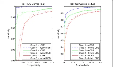
ROC curves were further used to evaluate the power of detecting change-points in the simulated data drawn from the Pearson System. A segment of copy number variations, 15 probes in width (k = 15), was embedded near the edges (l = 0) of every chromosome with 1,500 probes (N = 1,500). Successful detection of change-points from these data was defined as sensitivity. Cases without copy number variations were also tested for deriving specificity. Different settings of variation ampli-tudes, skewness, and kurtosis were tested, and the per-formance of the hybrid CBS and eCBS were compared using ROC curves.

Real aCGH Data

Two real aCGH datasets were employed to test the hybrid CBS and eCBS on computation time and seg-mentation accuracy. Ten unpublished breast cancer aCGH arrays using the Agilent Human Genome CGH 105A platform with 105,072 probes, were analyzed. Probes with unknown positions or small signal-to-noise ratios (SNR<1) were filtered out, and more than 93,000 probes in each array were left for data segmentation. Another aCGH dataset from GSE9177 (NCBI/GEO, 11 aCGH profiles of human glioblastoma GBM using the Agilent 244A human CGH arrays) were also down-loaded and processed for segmentation and performance comparison.

Results

Computation Time of the Hybrid CBS

In the breast cancer study with ten aCGH experiments, the percentage of time consumed by each critical step: candidate location, significance evaluation, and edge effect correction, are listed in Table 1. The results reveal that significance evaluation took at least 83% (93.7% on average) of the total time required to complete the seg-mentation process.

The GEV Distribution Models Maximal-tDistribution Adequately

To demonstrate whether the GEV distribution can model maximal-tdistribution well, we generated 10,000 random datasets under different distributions controlled

by skewness and kurtosis. The generated maximal-t dis-tribution was then fitted by maximum likelihood method with the GEV distribution. Figure 3 shows examples of maximal-t distribution and the fitted GEV distribution under three different conditions: (1) nor-mally distributed random data with 250 probes; (2) slightly skewed and heavy-tailed data with 400 probes; and (3) severely skewed and heavy-tailed data with 550 probes. The solid lines refer to the modeling GEV distri-bution while the dashed lines refer to the maximal-t dis-tribution. The results clearly demonstrate that the GEV distribution can adequately model maximal-t distribution.

The eXtreme Model Content Changes Smoothly

For a specific number of probesN, the eXtreme model provides three 2-dimensional tables, indexed by skew-ness and kurtosis, for the GEV parameters,g, s, and μ, respectively. Figure 4 shows an example of the tables in the eXtreme model withN= 200. With two parameters, namely, the skewnesss and kurtosis (estimated from aCGH data), an approximation of maximal-tdistribution in the form of the GEV parameters, g,s, and μ, can be quickly derived through the table lookup process. Addi-tionally, as shown in the figure, since the eXtreme model content changes smoothly, linear interpretation can be properly applied to provide an approximation when the query parameters (N,sk,ku) do not fall on the grid.

eCBS Performs Equivalently Comparing to the Hybrid CBS The performance of the eCBS algorithm was tested according to the simulation models described early. Using the second simulation model, it is revealed that eCBS has a negligible effect on change-points detection from data with normal noise. In Additional File 1: Sup-plementary Table, the“Exact” column accounts for the cases (among 1,000 simulations) that the segmentation results exactly match the desired number (1 for edge and 2 for center) and locations of change-points. As shown in the table, eCBS performed as good as the hybrid CBS wherever change-points were located. In addition, eCBS outperformed when the aberration width was small (k= 2).

eCBS Performs Adequately under Severely Skewed/Heavy-Tailed Conditions

2 2.5 3 3.5 4 4.5 5 5.5 6 6.5 7 0

0.2 0.4 0.6 0.8 1 1.2

Statistics

ksdensity

Modeling Maximal−t Distribution Using the GEV Distribution

Case 1 − Maximal−t Distribution Case 2 − Maximal−t Distribution Case 3 − Maximal−t Distribution

Case 1 − Max. Likelihood GEV Distribution Case 2 − Max. Likelihood GEV Distribution Case 3 − Max. Likelihood GEV Distribution

Figure 3The GEV distribution models maximal-tdistribution adequately. The maximum likelihood GEV distribution fitted maximal-t

distribution well. The dashed lines refer to the kernel smoothing density of the maximal-tstatistics derived from random numbers, and the solid lines are the maximum likelihood GEV distribution. Three examples under different conditions are shown in the figure. Case 1: number of probes

N= 250, skewnesssk= 0, kurtosisku= 3; Case 2:N= 400,sk= 0.5,ku= 4; and Case 3:N= 550,sk= 1,ku= 5.

0 0.5 1

3 4 5 −0.1 −0.05 0 0.05 0.1

skewness

(a) shape parameter

γ

kurtosis

γ

0 0.5 1

3 4 5 0.3 0.4 0.5

skewness

(b) scale parameter

σ

kurtosis

σ

0 0.5 1

3 4 5 3 3.2 3.4 3.6

skewness

(c) location parameter

μ

kurtosis

μ

distribution, and severely skewed/heavy-tailed distribu-tion. The simulation results shown in Figure 5 reveal that the difference between the hybrid CBS and eCBS is minimal.

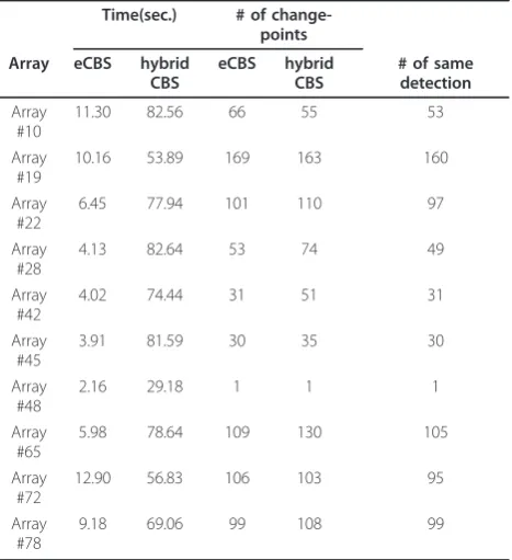
eCBS Performs 4× to 20× Faster than the Hybrid CBS To study the performance of eCBS in terms of the speed, ten breast cancer aCGH arrays were analyzed by both the hybrid CBS and eCBS, and the total time con-sumed on segmentation was compared and listed in Table 2. The time consumed on the pre-segmentation was taken into consideration when eCBS was applied. As shown in the table, it took eCBS much less computa-tion time for segmenting: only about 10 seconds were required to analyze a dataset with eCBS, while on aver-age, 68.68 seconds were needed for the hybrid CBS. The performance of eCBS in speed can be 4-fold faster, or even better. Taking arrays #28 and #45 for example, eCBS performed 20-fold faster than the hybrid CBS.

The segmentation results for eCBS were slightly differ-ent from those of the hybrid CBS. In samples #10, #19 and #72, eCBS detected more change-points than the hybrid CBS, while in the other experiments, eCBS

detected fewer change-points. However, the segmenta-tion results were mostly the same. The eCBS algorithm was also applied to a GSE9177 dataset of GBM samples. As shown in Table 3, eCBS performed four times faster than the hybrid CBS.

Discussion

Circular Binary Segmentation (CBS) performs consis-tently in detecting change-points and thus provides us a good framework for further improvements. The frame-work of CBS is mainly constituted of three steps: candi-date location, significance evaluation, and edge effect correction. The first step, candidate location, locates candidate change-points by a maximal-tstatistic. The second step, significance evaluation, approximates the significance of change-points by permutations or a hybrid method; the last step, edge effect correction, removes errors near the edges due to a circling process. Of these steps, significance evaluation was the major component that made the algorithm time-consuming. A time consumption study (shown in Table 1) on the hybrid CBS that involved analyzing ten breast cancer microarrays supported the above statement: among the

0 0.01 0.02 0.03 0.04 0.05

0.95 0.96 0.97 0.98 0.99 1

1−specificity

sensitivity

(a) ROC Curves (c=2)

0 0.05 0.1 0.15 0.2

0.3 0.4 0.5 0.6 0.7 0.8 0.9 1

1−specificity

sensitivity

(b) ROC Curves (c=1.5)

Case 1 − eCBS Case 1 − hybrid CBS Case 2 − eCBS Case 2 − hybrid CBS Case 3 − eCBS Case 3 − hybrid CBS Case 1 − eCBS

Case 1 − hybrid CBS Case 2 − eCBS Case 2 − hybrid CBS Case 3 − eCBS Case 3 − hybrid CBS

Figure 5The comparison of ROC curves between the hybrid CBS and eCBS. The ROC curves obtained from the segmentation results of 10,000 simulated datasets. Each dataset contained 1,500 probes. Case 1 refers to the performance of analyzing normally distributed data withsk

ten experiments, up to 98% of time consumed was attri-butable to significance evaluation, in which permuta-tions took the majority of the time for evaluating p-values, even when early stopping rules were applied. To improve the performance of the hybrid CBS in speed,

we significantly reduce computation time using the eXtreme model.

The eXtreme model contains lookup tables which associates characteristics of aCGH data with the para-meters of GEV distribution. The simulation, which applied the Pearson system to generate synthetic aCGH data, was done in advance rather than invoked on demand, such as the permutations for the hybrid CBS. Since maximal-tdistribution is sensitive to heavy tails and outliers (shown in Figure 2), non-normal aCGH data distribution was considered for the simulation. Thousands of non-normal aCGH data under null hypothesis (without change-points) were simulated. The corresponding maximal-tdistribution was then modeled by the GEV distribution, and the modeling results in the form of the GEV parameters,g,s, andμ, were saved in the eXtreme model (lookup tables).

Using the eXtreme model, maximal-tdistribution can be approximated given the estimates of skewness (sk) and kurtosis (ku) from the aCGH data and the number of probes (N) under consideration. If the input para-meters (sk, ku,N) fall right on the table grid, the output GEV parameters (g,s,μ) are directly derived through a table lookup process. Otherwise, since the table content changes smoothly (shown in Figure 4), linear interpola-tion from eight closest points in the 3-dimensional tables was applied. Through the table lookup process, maximal-tdistribution and the subsequent approxima-tion of the significance of change-points can be evalu-ated inO(1).

Deriving robust estimates of skewness and kurtosis from aCGH data is a critical step before using the eXtreme model, since estimating bias and variations may lead to incorrect approximations of maximal-t dis-tribution and increase false positive or negative. In addi-tion to the noise from microarray experiments, CNAs greatly increase the difficulties in estimating these para-meters. Recognized what we needed here were estimates of skewness and kurtosis under null condition (the con-dition rarely exists because there are always CNAs within tumor samples), we selected a pre-segmentation step (see Additional File 1: Supplementary Materials) to rapidly pre-cut large regions of amplification or deletion. After removing the mean values of gain and loss seg-ments, skewness and kurtosis can be accurately estimated.

Based on the eXtreme model, a novel algorithm, eCBS, has been developed. First, eCBS pre-segments data and estimates the skewness and kurtosis from the aCGH data. These estimates will be utilized later by the eXtreme model to provide approximations of maximal-t distribution. Once the estimates are provided, eCBS detects the maximal statistic, Tmax, and locates candi-date change-points in a similar way operated by CBS. Table 2 Comparison of performance in speed using the

hybrid CBS and eCBS - 1

Time(sec.) # of change-points

Array eCBS hybrid CBS

eCBS hybrid CBS

# of same detection

Array #10

11.30 82.56 66 55 53

Array #19

10.16 53.89 169 163 160

Array #22

6.45 77.94 101 110 97

Array #28

4.13 82.64 53 74 49

Array #42

4.02 74.44 31 51 31

Array #45

3.91 81.59 30 35 30

Array #48

2.16 29.18 1 1 1

Array #65

5.98 78.64 109 130 105

Array #72

12.90 56.83 106 103 95

Array #78

9.18 69.06 99 108 99

The computation time and segmentation results using the hybrid CBS and eCBS in a breast cancer study with 10 aCGH experiments. The time consumed in pre-segmentation was taken into consideration when eCBS was applied.

Table 3 Comparison of performance in speed using the hybrid CBS and eCBS - 2

Time(sec.) # of change-points

Array eCBS hybrid

CBS

eCBS hybrid CBS

# of same detection

GSM231848 52.26 226.7 557 607 531

GSM231849 62.27 227.5 1208 1217 1118

GSM231850 78.48 203.8 2383 2577 2296

GSM231851 43.87 166.8 123 117 109

GSM231852 57.34 181.0 101 142 100

GSM231853 41.62 259.2 455 520 420

GSM231854 53.16 245.0 968 1010 920

GSM231855 49.91 249.1 1091 1174 1017

*GSM231856 32.09 297.8 291 625 291

GSM231857 91.86 223.2 2163 2116 2041

GSM231858 94.39 203.1 2476 2483 2376

Please note that the maximal-tstatistic is derived from the original aCGH data, not from the data after pre-seg-mentation. After candidate change-points are located, thep-value, or the significance of change-points, is eval-uated based on the maximal-tdistribution approximated using the eXtreme model. After edge effect correction further removes errors due to the circling process, change-points and the consequent subsegments are found. The process of finding change-points repeats iteratively until no more change-points can be detected. Rather than providing an upper bound or a lower bound ofp-values, as implemented in the hybrid CBS, eCBS outperforms the hybrid CBS by approximating p-values forTmaxdirectly and reducing required permuta-tions for significance evaluation.

Conclusions

A novel algorithm, eCBS, was developed in this study, in which the significance of change-points is evaluated using the eXtreme model. The eXtreme model provides approximations of maximal-tdistribution for hypothesis testing. With limited utilization of permutations, eCBS evaluates the significance of change-points through a table lookup process and achieves the best performance in speed. Via real aCGH data analysis and simulations, we showed that eCBS can perform as robustly as CBS, but with much less computation time. The eCBS algo-rithm with eXtreme model was implemented in an R package and is available from the supplementary website.

Availability and Requirements

The eCBS algorithm was developed using Linux (version 2.6.11-1.1369 FC4smp) and R (version 2.8.0), and the source code is freely available at http://ntumaps.cgm. ntu.edu.tw/eCBSsupplementary. In order to execute properly, a compatible version of Linux operating sys-tem with R environment is required. Installation instruc-tions are included in the manual (\eCBS\inst\doc\eCBS. pdf).

Additional material

Additional file 1: This additional file contains supplementary materials, supplementary figures and supplementary tables.

Acknowledgements and Funding

The authors would like to thank the members in the Bioinformatics and Biostatistics Core Laboratory, Center for Genomic Medicine, National Taiwan University, for helpful discussions. This research was supported in part by NCI/NIH Cancer Center Grant P30 CA054174-17 (Y.C.), NIH/NCRR 1UL1RR025767-01 (Y.C.), 95HM0033195R0066-BM01-01 (E.Y.C.) and 98R0065 (E.Y.C.) from National Taiwan University, and DOH98-TD-G-111-003 (E.Y.C.) from the Department of Health, Executive Yuan, ROC (Taiwan). The funding

agencies had no role in study design, data collection and analysis, decision to publish, or preparation of the manuscript.

Author details 1

Graduate Institute of Biomedical Electronics and Bioinformatics, Department of Electrical Engineering, National Taiwan University, Taipei 106, Taiwan. 2

Greehey Children’s Cancer Research Institute, The University of Texas Health Science Center at San Antonio, San Antonio, TX 78229, USA.3_{Department of} Epidemiology and Biostatistics, The University of Texas Health Science Center at San Antonio, San Antonio, TX 78229, USA.4_{Institute of Biotechnology,} Center for Systems Biology and Bioinformatics, National Taiwan University, Taipei 106, Taiwan.5_{Graduate Institute of Physiology, National Taiwan} University, Taipei 100, Taiwan.6_{Cathy General Hospital, Taipei 106, Taiwan.}

Authors_’contributions

FH, HC, and YC designed the eCBS algorithm and carried out the performance analysis. CH and ST collected the samples of breast cancer tissue. EC, MT and LL designed and participated in the coordination of microarray experiments. All authors collectively wrote the paper, read and approved the final manuscript.

Competing interests

The authors declare that they have no competing interests.

Received: 2 June 2011 Accepted: 10 October 2011 Published: 10 October 2011

References

1. Beckmann JS, Estivill X, Antonarakis SE:Copy number variants and genetic traits: closer to the resolution of phenotypic to genotypic variability.

Nature Reviews Genetics2007,8(8):639-646.

2. Monni O, Barlund M, Mousses S, Kononen J, Sauter G, Heiskanen M, Paavola P, Avela K, Chen Y, Bittner ML, Kallioniemi A:Comprehensive copy number and gene expression profiling of the 17q23 amplicon in human breast cancer.PNAS2001,98(10):5711..

3. Wolf M, Mousses S, Hautaniemi S, Karhu R, Huusko P, Allinen M, Elkahloun A, Monni O, Chen Y, Kallioniemi A, Kallioniemi OP: High-resolution analysis of gene copy number alterations in human prostate cancer using CGH on cDNA microarrays: impact of copy number on gene expression.Neoplasia (New York, NY)2004,6(3):240.

4. Pinkel D, Albertson DG:Array comparative genomic hybridization and its applications in cancer.Nature Genetics2005,37:S11-S17.

5. Davies JJ, Wilson IM, Lam WL:Array CGH technologies and their applications to cancer genomes.Chromosome research2005, 13(3):237-248.

6. Wang P, Kim Y, Pollack J, Narasimhan B, Tibshirani R:A method for calling gains and losses in array CGH data.Biostatistics2005, 645.

7. Fridlyand J, Snijders AM, Pinkel D, Albertson DG, Jain AN:Hidden Markov models approach to the analysis of array CGH data.Journal of Multivariate Analysis2004,90:132-153.

8. Marioni JC, Thorne NP, Tavare S:BioHMM: a heterogeneous hidden Markov model for segmenting array CGH data.Bioinformatics2006, 22(9):1144.

9. Pique-Regi R, Monso-Varona J, Ortega A, Seeger RC, Triche TJ,

Asgharzadeh S:Sparse representation and Bayesian detection of genome copy number alterations from microarray data.Bioinformatics2008, 24(3):309.

10. Wu LY, Chipman HA, Bull SB, Briollais L, Wang K:A Bayesian segmentation approach to ascertain copy number variations at the population level.

Bioinformatics2009,25(13):1669.

11. Olshen AB, Venkatraman ES, Lucito R, Wigler M:Circular binary segmentation for the analysis of array-based DNA copy number data.

Biostatistics2004,5(4):557.

12. Willenbrock H, Fridlyand J:A comparison study: applying segmentation to array CGH data for downstream analyses.Bioinformatics2005,21(22):4084. 13. Lai WR, Johnson MD, Kucherlapati R, Park PJ:Comparative analysis of

algorithms for identifying amplifications and deletions in array CGH data.Bioinformatics2005,21(19):3763.

Hurles ME, Edwards PAW, Bignell GR, Stratton MR, Futreal PA:Identification of somatically acquired rearrangements in cancer using genome-wide massively parallel paired-end sequencing.Nature genetics2008, 40(6):722-729.

15. Deshmukh H, Yeh TH, Yu J, Sharma MK, Perry A, Leonard JR, Watson MA, Gutmann DH, Nagarajan R:High-resolution, dual-platform aCGH analysis reveals frequent HIPK2 amplification and increased expression in pilocytic astrocytomas.Oncogene2008,27(34):4745-4751. 16. Venkatraman ES, Olshen AB:A faster circular binary segmentation

algorithm for the analysis of array CGH data.Bioinformatics2007, 23(6):657.

17. Network TCGA:Integrated genomic analyses of ovarian carcinoma.

Nature2011,474:609.

18. Kim TH, White H:On more robust estimation of skewness and kurtosis.

Finance Research Letters2004, 156-73.

19. Hardin J, Wilson J:A note on oligonucleotide expression values not being normally distributed.Biostatistics2009,10(3):446.

20. Andreev A, Kanto A, Malo P:Simple approach for distribution selection in the Pearson system.Helinski School of Economics-Electronic Working Papers

2005,388:22.

21. Stuart A, Ord JK:Kendall’s advanced theory of statistics. Vol. 1 Distribution theoryHodder Arnold; 1994.

22. Embrechts P, Schmidli H:Modelling of extremal events in insurance and finance.Mathematical Methods of Operations Research1994,39:1-34. 23. Jenkinson AF:The frequency distribution of the annual maximum (or

minimum) values of meteorological elements.Quarterly Journal of the Royal Meteorological Society1955,81(348):158-171.

24. Von Mises R:La distribution de la plus grande de n valeurs. Reprinted in Selected Papers Volumen II.American Mathematical Society, Providence, RI

1954, 271-294.

25. Gilleland E, Katz RW:Tutorial for The‘Extremes Toolkit: Weather and Climate Applications of Extreme Value Statistics.[http://www.assessment. ucar.edu/toolkit, 2005].

26. Gupta C:Statistical properties of chaotic dynamical systems: extreme value theory and Borel-Cantelli Lemmas.PhD thesisUniversity of Houston; 2010.

doi:10.1186/1756-0500-4-394

Cite this article as:Hsuet al.:A model-based circular binary segmentation algorithm for the analysis of array CGH data.BMC Research Notes20114:394.

Submit your next manuscript to BioMed Central and take full advantage of:

• Convenient online submission

• Thorough peer review

• No space constraints or color figure charges

• Immediate publication on acceptance

• Inclusion in PubMed, CAS, Scopus and Google Scholar

• Research which is freely available for redistribution