City, University of London Institutional Repository
Citation
:
França, M. V. M., Zaverucha, G. and Garcez, A. (2014). Fast relational learning using bottom clause propositionalization with artificial neural networks. Machine Learning, 94(1), pp. 81-104. doi: 10.1007/s10994-013-5392-1This is the unspecified version of the paper.
This version of the publication may differ from the final published
version.
Permanent repository link:
http://openaccess.city.ac.uk/3057/Link to published version
:
http://dx.doi.org/10.1007/s10994-013-5392-1Copyright and reuse:
City Research Online aims to make research
outputs of City, University of London available to a wider audience.
Copyright and Moral Rights remain with the author(s) and/or copyright
holders. URLs from City Research Online may be freely distributed and
linked to.
City Research Online: http://openaccess.city.ac.uk/ [email protected]
Fast Relational Learning using Bottom Clause
Propositionalization with Artificial Neural Networks
Manoel V. M. França Gerson Zaverucha Artur S. d’Avila Garcez
July 15, 2013
Abstract
Relational learning can be described as the task of learning first-order logic rules from examples. It has enabled a number of new machine learning applications, e.g. graph min-ing and link analysis. Inductive Logic Programmmin-ing (ILP) performs relational learnmin-ing either directly by manipulating first-order rules or through propositionalization, which translates the relational task into an attribute-value learning task by representing subsets of relations as features. In this paper, we introduce a fast method and system for relational learning based on a novel propositionalization called Bottom Clause Propositionalization (BCP). Bottom clauses are boundaries in the hypothesis search space used by ILP systems Progol and Aleph. Bottom clauses carry semantic meaning and can be mapped directly onto numerical vectors, simplifying the feature extraction process. We have integrated BCP with a well-known neural-symbolic system, C-IL2P, to perform learning from nu-merical vectors. C-IL2P uses background knowledge in the form of propositional logic programs to build a neural network. The integrated system, which we call CILP++, han-dles first-order logic knowledge and is available for download from Sourceforge. We have evaluated CILP++ on seven ILP datasets, comparing results with Aleph and a well-known propositionalization method, RSD. The results show that CILP++ can achieve accuracy comparable to Aleph, while being generally faster, BCP achieved statistically significant improvement in accuracy in comparison with RSD when running with a neural network, but BCP and RSD perform similarly when running with C4.5. We have also extended CILP++ to include a statistical feature selection method, mRMR, with preliminary re-sults indicating that a reduction of more than 90% of features can be achieved with a small loss of accuracy.
Keywords:Relational Learning, Inductive Logic Programming, Propositionalization, Neural-Symbolic Integration, Artificial Neural Networks
1
Introduction
Muggleton et al., 2010). Inductive Logic Programming (ILP) (Muggleton and Raedt, 1994; Nienhuys-Cheng and de Wolf, 1997) performs relational learning either directly by manipulat-ing first-order clauses or through a method called propositionalization (Lavraˇc and Džeroski, 1994; Železný and Lavraˇc, 2006), which brings the relational task down to the propositional level by representing subsets of relations as features that can then be used as attributes. In com-parison with full ILP, propositionalization normally exchanges accuracy for efficiency (Krogel et al., 2003), as it enables the use of fast attribute-value learners such as decision trees or even neural networks (Quinlan, 1993; Rumelhart et al., 1994), but could lose information in the translation of first-order clauses into features.
In this paper, we introduce a fast system for relational learning based on a new form of propositionalization, which we call Bottom Clause Propositionalization (BCP). Bottom clauses are boundaries on the hypothesis search space, first introduced by Muggleton (1995) as part of the Progol system, and are built from one random positive example, background knowledge (a set of clauses that describe what is known) and language bias (a set of clauses that define how clauses can be built). A bottom clause is the most specific clause (with most literals) that can be considered as a candidate hypothesis. BCP uses bottom clauses for propo-sitionalization because they carry semantic meaning, and because bottom clause literals can be used directly as features in a truth-table, simplifying the feature extraction process (Muggleton and Tamaddoni-Nezhad, 2008; DiMaio and Shavlik, 2004; Pitangui and Zaverucha, 2012).
The idea of using BCP for learning came from our attempts to represent and learn first-order logic in neural networks (Garcez and Zaverucha, 2012). Neural networks (Rumelhart et al., 1994) are attribute-value learners based on gradient-descent. Learning in neural net-works is achieved by performing small changes to a set of weights, in contrast with ILP, which performs learning at the concept level. Neural networks’ distributed architecture is generally accredited as a reason for robustness; neural networks seem to perform well in continuous domains and when learning from noisy data (Rumelhart et al., 1994). Systems that com-bine symbolic computation with neural networks are called neural-symbolic systems (Garcez et al., 2002). In neural-symbolic integration, the representation of first-order logic by neural networks is of interest in its own right, since first-order logic learning and reasoning using connectionist systems remains an open research question (Garcez et al., 2008). As a result, we investigate whether neural-symbolic learning is a good match for BCP. The experiments reported below indicate that this is indeed the case, in comparison with standard ILP and a well-known propositionalization method.
The neural-symbolic system C-IL2P has been shown effective at learning and reasoning from propositional data in a number of domains (Garcez and Zaverucha, 1999). C-IL2P uses background knowledge in the form of propositional logic programs to build a neural network, which is in turn trained by examples using backpropagation (Rumelhart et al., 1994). We in-tend to achieve the same in relational domains. Hence, we have exin-tended C-IL2P to handle first-order logic by using BCP to train a first-order neural network. The extended system, which we call CILP++, has been implemented in C++ and is available to download from
summarised in the next paragraph, our long-term goal is to apply and evaluate BCP on other general settings, including discrete and continuous data, noisy environments with missing val-ues, and problems containing errors in the background knowledge.
We have compared CILP++ with Aleph (Srinivasan, 2007) – a state-of-the-art ILP system based on Progol – and compared BCP with a well-known propositionalization method, RSD (Železný and Lavraˇc, 2006), using neural networks and the C4.5 decision tree learner (Quin-lan, 1993), on a number of benchmarks: fourAlzheimer’sdatasets (King and Srinivasan, 1995) and theMutagenesis(Srinivasan and Muggleton, 1994),KRK(Bain and Muggleton, 1994) and
UW-CSE(Richardson and Domingos, 2006) datasets. Several aspects were empirically evalu-ated: standard classification accuracy using cross-validation and runtime measurements, how BCP performs in comparison with RSD, and how CILP++ performs in different settings us-ing feature selection (Guyon and Elisseeff, 2003). The CILP++ implementation has not been optimised for performance. We evaluated six different configurations of CILP++ in order to explore some of the capabilities of the approach: three versions of CILP++ trained with standard backpropagation, each one using three sizes of background knowledge, and three versions of CILP++ trained with early stopping (Prechelt, 1997), with the same three back-ground knowledge sizes used for standard backpropagation. In the first set of experiments – accuracy vs. runtime – CILP++ achieved results comparable to Aleph and performed faster on most datasets.
Regarding the performance of BCP against RSD, BCP achieved a statistically significant improvement in accuracy in comparison with RSD when running with a neural network, but BCP and RSD have shown similar performance when running with C4.5. Nevertheless, BCP was faster than RSD in all cases. Since bottom clauses may have a large number of literals (Muggleton, 1995), BCP might generate a large number of features. Hence, we evaluated ac-curacy also using feature selection, as follows. CILP++ was extended to include a statistical feature selection method called mRMR which is widely used for visual recognition and audio analysis (Ding and Peng, 2005). We applied three-fold cross validation on training data to choose two models and used those on twoAlzheimer datasets. The results indicate the exis-tence of an optimal variable-depth parameter for generating bottom clauses and that “more is not merrier”. In one CILP++ model, mRMR managed to reduce over 90% of features while having a loss of less than 2% on accuracy on twoAlzheimertestbeds, although an increase in runtime was observed. Further experiments in different application domains and comparison with other propositionalization methods, e.g. Kuželka and Železný (2011), are under way.
Related Work: Approaches related to CILP++ can be grouped into three categories: ap-proaches that also use bottom clauses, other propositionalization methods, and other relational learning methods. In the first category, DiMaio and Shavlik (2004) use bottom clauses with neural networks to build an efficient hypothesis evaluator for ILP. Instead, CILP++ uses bot-tom clauses to classify first-order examples. The QG/GA system (Muggleton and Tamaddoni-Nezhad, 2008) introduces a new hypothesis search algorithm for ILP, called Quick Generaliza-tion (QG), which performs random single reducGeneraliza-tions in bottom clauses to generate candidate clauses for hypothesis. Additionally, QG/GA proposes the use of Genetic Algorithms (GA) on those candidate clauses to further explore the search space, converting the clauses into nu-merical patterns. CILP++ does the same, but for use with neural networks instead of discrete GAs.
successor, DINUS (Kramer et al., 2001), allows a larger subset of clauses to be accepted (determinate clauses), allowing clauses with body variables that do not appear in the head literal, but still allowing only one possible instantiation of those variables. Finally, SINUS (Kramer et al., 2001) improved on DINUS by allowing unconstrained clauses, making use of language bias in the feature selection and verifying if it is possible to unify newly found literals with existing ones, while keeping consistency between pre-existing variable namings, thus reducing the final number of features. LINUS and DINUS treat body literals as features, which is similar to BCP. However, BCP can deal with the same language as Progol, thus having none of the language restrictions of LINUS/DINUS. SINUS, on the other hand, propositionalizes similarly to another method, RSD, which is compared to this work and is explained separately in Section 2.3. RSD also has a recent successor, called RelF (Kuželka and Železný, 2011), which takes a more classification-driven approach than RSD by only considering features that are interesting for distinguishing between classes (it also discards features thatθ-subsumeany previously-generated feature). Comparisons with RelF are under way.
Finally, in the third category, we place the body of work on statistical relational learning (Getoor and Taskar, 2007; De Raedt et al., 2008), that albeit relevant for comparison, is less directly related to this work, e.g. Markov Logic Networks (MLN) (Richardson and Domingos, 2006) and other systems combining relational and probabilistic graphical models (Koller and Friedman, 2009; Paes et al., 2005), neural-symbolic systems for learning from first-order data in neural networks such as Basilio et al. (2001), Kijsirikul and Lerdlamnaochai (2005) and Guillame-Bert et al. (2010), and systems that propose to integrate neural networks and first-order logic through relational databases, e.g. Uwents et al. (2011). Those systems differ from CILP++ mainly in that they seek to embed relational data directly into the networks’ structures, which is a difficult task. In contrast, CILP++ seeks to benefit from using a simple network structure as an attribute-value learner, following a propositionalization approach, as discussed earlier.
Summarizing, the contribution of this paper is two-fold. The paper introduces: (i)a novel propositionalization method, BCP, which converts first-order examples into propositional pat-terns by generating their bottom clauses, treating each body literal as a propositional feature, and (ii)the successor of C-IL2P, the CILP++ system, which reduces C-IL2P’s learning times and system complexity, uses a new weight normalization, maintaining the integrity of first-order background knowledge, and is easily configurable to be used with any ILP dataset. CILP++ takes advantage of mode declarations and determinations to generate consistent bot-tom clauses which share variable namings, thus being applicable to any dataset that first-order systems Aleph or Progol are applicable. CILP++ may use C-IL2P’s knowledge extraction al-gorithm (Garcez et al., 2001) so that interpretable first-order rules can be obtained from the trained network. Currently, first-order rules can be obtained when BCP is used together with C4.5 (since each node represents a first-order literal). This is further discussed in the body of the paper.
2
Background
In this section, both machine learning subfields that are directly related to this work (In-ductive Logic Programming and Artificial Neural Networks) are reviewed. This section also introduces notation used throughout the paper. An introduction to C-IL2P is also presented, followed by a review of propositionalization and feature selection.
2.1 ILP and Bottom Clause
Inductive Logic Programming (Muggleton and Raedt, 1994) is an area of machine learning that makes use of logical languages to induce theory-structured hypotheses. Given a set of labeled examplesEand background knowledgeB, an ILP system seeks to find a hypothesisH
that minimizes a specified loss function. More precisely, an ILP task is defined as<E, B, L>, whereE=E+ ∪E−is a set of positive (E+) and negative (E−) clauses, calledexamples,Bis a logic program calledbackground knowledge, which is composed byfactsandrules, andLis a set of logic theories calledlanguage bias.
The set of all possible hypotheses for a given task, which we call SH, can be infinite
(Muggleton, 1995). One of the features that constrainsSHin ILP is the language bias,L. It is
usually composed by specification predicates, which define how the search is done and how far it can go. The most common specification language is calledmode declarations, composed of: modeh predicates, that define what can appear as head of a clause; modeb predicates, that define what predicates can appear in the body of a clause; anddeterminationpredicates, which relate body and head literals. The modebandmodeh declarations also specify what is considered to be an input variable, an output variable, a constant, and an upper bound on how many times the predicate it specifies can appear in the same clause, called recall. The language bias L, through mode declarations and determination predicates, can restrict
SH during hypothesis search to only allow a smaller set of candidate hypotheses Hc to be
searched. Formally,Hcis a candidate hypothesis for a given ILP task <E, B, L>iffHc∈L,
B∪HcE+∪N andB∪Hc2E−−N, whereN⊆E− is an allowednoiseinHc in order to
ameliorate overfitting issues.
Something else that is used to restrict hypothesis search space in algorithms based on in-verse entailment, such as Progol, is themost specific (saturated) clause,⊥e. Given an example
e, Progol firstly generates a clause that representsein the most specific way as possible, by searching inLfor modehdeclarations that can unify withe and if it finds one, an initial⊥e
is created. Then it passes through thedeterminationpredicates to verify which of the bodies specified among the modebclauses can be added to⊥e, repeatedly, until a number of cycles
(known asvariable depth) through themodebdeclarations has been reached.
2.2 Artificial Neural Networks and C-IL2P
An artificial neural network (ANN) is a directed graph with the following structure: a unit (or neuron) in the graph is characterized, at time t, by its input vector Ii(t), its input
potential Ui(t), itsactivation state Ai(t), and itsoutput Oi(t). The units of the network are
interconnected via a set of directed and weighted connections such that if there is a connection from unitito unit jthenWji∈Rdenotes theweightof this connection. The input potential of neuroniat timet(Ui(t)) is obtained by computing a weighted sum for neuronisuch that
Ui(t) =∑jWi jIi(t). The activation stateAi(t)of neuroniat timetis then given by the neuron’s
always fixed at 1) is known as thebiasof neuroni. We say that neuroniisactiveat timet if
Ai(t)>−bi.Finally, the neuron’s output value is given by its activation stateAi(t).
For learning,backpropagation(Rumelhart et al., 1994) is the most widely used algorithm, based on gradient descent. It aims to minimize an error function Eregarding the difference between the network’s answer and the example’s actual classification. Standard trainingand
early stopping(Haykin, 2009) are two commonly used stopping criteria for backpropagation training. In standard training, the full training dataset is used to minimize E, while early stopping uses a validation set to measure data overfitting: training stops when the validation set error starts to increase. When this happens, the best validation configuration obtained thus far is used as the learned model.
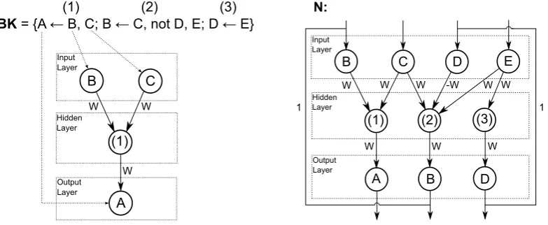
The Connectionist Inductive Learning and Logic Programming system, C-IL2P (Garcez and Zaverucha, 1999), is a neural-symbolic system that builds a recursive ANN using back-ground knowledge composed of propositional clauses (building phase). C-IL2P also learns from examples using backpropagation (training phase), performs inference on unknown data by querying the post-training ANN, and extracts a revised knowledge from the trained network (Garcez et al., 2001) to obtain a new propositional theory (extraction phase). Fig. 1 illustrates the building phase and shows how to build a recursive ANN Nfrom background knowledge BK1.
BK = {A ← B, C; B ← C, not D, E; D ← E}
Input Layer Hidden Layer Output Layer B C (1) A (1) (2) (3)
W W W N: Input Layer Hidden Layer Output Layer
B C D E
A B D (1) (2) (3)
W W W -W W W
W W W
[image:7.595.104.496.351.512.2]1 1
C-IL2P calculates weight and bias values for all neurons. The value ofW is constrained by Eq. 2, the values of the biases of the input layer neurons are set as 0, and the biases of the hidden layer neurons nh (bnh) and of the output layer neuronsno(bno) are given by Eqs. 3 and 4 below, respectively. Both W and the biases are functions of Amin: this parameter
controls the activation of each neuronnin C-IL2P by only allowing activation if the condition shown in Eq. 1 is satisfied, where wi is a network weight that ends inn, xi is an input and
hn is the activation function of neuronn, which islinear if it is an input neuron and
semi-linear bipolar2 if it is not. W and the biases values are set so that the network implements an AND-OR structure with hidden neurons implementing a logical-AND of input neurons, and output neurons implementing a logical-OR of hidden neurons, so that the network can be used to run the logic program. To exemplify the network computation, givenBK, if E and C are set to true, and D is set to false in the network (i.e. neurons E and C are activated while neuron D is not), a feedforward propagation activates output neuron B (because of the second clause in BK). Then, a recursive connection carries this activation to input neuron B, and a second feedforward propagation would activate A. This process continues until a stable state is reached, when no change in activation is seen after a feedforward propagation.
hn(
∑
∀i
wi·xi+b)≥Amin (1)
W≥ 2
β ·
ln(1+Amin)−ln(1−Amin)
max(kn,µn)·(Amin−1) +Amin+1
(2)
bnh=
(1+Amin)(knh−1)
2 ·W (3)
bno =
(1+Amin)(1−µno)
2 ·W (4)
In Eqs. 2, 3 and 4: knh is the number of body literals in the clause corresponding to the hidden neuron nh (i.e., the number of connections coming from the input layer to nh); µno is the number of clauses in the background knowledge with the same head as the head literal mapped by the output neuronno(i.e., the number of connections coming from the hidden layer
tono);max(kn,µn)is the maximum value among allkand allµ, for all neuronsn; andβ is the
semi-linear bipolaractivation function slope.
After the building phase, training can take place. Optionally, more hidden neurons can be added (if this is needed in order to better approximate the training data), and the network is fully connected with near-zero weighted connections. The training algorithm used by C-IL2P is standard backpropagation (Rumelhart et al., 1994). C-IL2P also does not train recursive connections: they are fixed and only used for inference.
Then, inference and knowledge extraction can be done. Garcez et al. (2001) proposes a knowledge extraction algorithm for C-IL2P by splitting of the trained network into “regular” ones, which do not have connections coming from the same neuron with different signs (pos-itive and negative). It is shown that the extraction for those networks is sound and complete, and in the general case, soundness can be achieved, but not completeness.
1We follow logic programming notation where a clause of the form (A←B, not C, D) denotes that A is true if B is true, C is false and D is true; clauses are separated by “;” (semi-colon) in a logic program.
2Semi-linear bipolar function: f(x) = 2
2.3 Propositionalization
Propositionalization is the conversion of a relational database into an attribute-value table, amenable to conventional propositional learners (Krogel et al., 2003). Propositionalization algorithms use background knowledge and examples to find distinctive features, which can differentiate subsets of examples. There are two kinds of propositionalization: logic-oriented
anddatabase-oriented. The former aims to build a set of relevant first-order features by distin-guishing between first-order objects. The latter aims to exploit database relations and functions to generate features for propositionalization. The main representatives oflogic-oriented ap-proaches include: LINUS (and its successors), RSD and RelF; and the main representative of
database-orientedapproaches is RELAGGS (Krogel and Wrobel, 2003). BCP is a new logic-orientedpropositionalization technique, which consists of generating bottom-clauses for each first-order example and using the set of all body literals that occur in them as possible features (in other words, as columns for an attribute-value table).
In order to evaluate how BCP performs, it will be compared with RSD (Železný and Lavraˇc, 2006), a well-known propositionalization algorithm for which an implementation is available at (http://labe.felk.cvut.cz/~zelezny/rsd). RSD is a system which tackles the Relational Subgroup Discoveryproblem: given a population of individuals and a property of interest, RSD seeks to find population subgroups that are as large as possible and have the most unusual distribution characteristics. RSD’s input is an Aleph-formatted dataset, with background knowledge, example set and language bias and its output is a list of clauses that describe interesting subgroups of the examples dataset. RSD is composed of two steps: first-order feature construction and rule induction. The first is a propositionalization method that creates higher-level features that are used to replace groups of first-order literals, and the second is an extension of the propositional CN2 rule learner (Clark and Niblett, 1989), for use as a solver of the relational subgroup discovery problem. We are interested in the proposition-alization component of RSD, which can be further divided into three steps: all expressions that by definition form a first-order feature and comply with the mode declarations are iden-tified; the user can instantiate variables (through instantiate/1predicates) in the background knowledge and afterwards, irrelevant features are filtered out; and a propositionalization of each example using the generated features is created. From now on, when we refer to RSD, we are referring to the RSD propositionalization method, not the relational subgroup discovery system.
2.4 Feature Selection
I between variablesxandy, defined as:
I(x,y) =
∑
i,j
p(xi,yj)log
p(xi,yj)
p(xi)p(yj)
, (5)
wherep(x,y)is the joint probability distribution, andp(x)andp(y)are the respective marginal probabilities. Given a subset S of the feature set Ωto be ranked by mRMR, the minimum redundancy condition and the maximum relevance condition, respectively, are:
min{WI},WI=
1
|S|2
∑
i,j∈S
I(i,j)and (6)
max{VI},VI=
1
|S|
∑
i∈SI(h,i), (7)whereh={h1,h2, . . . ,hK}is the classification variable of a dataset withKpossible classes. Let
ΩS=Ω−Sbe the set of unselected features fromΩ. There are two ways of combining the two
conditions above to select features fromΩS: Mutual Information Difference (MID), defined
as max(VI−WI), and Mutual Information Quotient (MIQ), defined as max(VI/WI). Results
reported in Ding and Peng (2005) indicate that MIQ usually chooses better features. Thus, MIQ is the function we choose to select features in this work and for the sake of simplicity, whenever this work refers to mRMR, it is referring to mRMR with MIQ.
3
Learning with BCP using CILP++
Let us start with a motivating example: consider the well-known family relationship ex-ample (Muggleton and Raedt, 1994), with background knowledgeB= {mother(mom1, daugh-ter1),wife(daughter1, husband1),wife(daughter2, husband2)}, with positive example moth-erInLaw(mom1, husband1), and negative examplemotherInLaw(daughter1, husband2). It can be noticed that the relation betweenmom1andhusband1, which the positive example estab-lishes, can be alternatively described by the sequence of factsmother(mom1, daughter1)and
wife(daughter1, husband1)in the background knowledge. This states semantically thatmom1
is a mother-in-law because mom1 has a married daughter, namely, daughter1. Applied to this example, the bottom clause generation algorithm of Progol would create a clause ⊥=
motherInLaw(A,B) ← mother(A, C), wife(C, B). Comparing ⊥ with the sequence of facts above, we notice that ⊥ describes one possible meaning of mother-in-law: “A is a mother-in-law of BifAis a mother ofC andC is wife ofB”, i.e. the mother of a married daughter is a mother-in-law. This is why, in this paper, we investigate learning from bottom clauses. However, for each learned clause, Progol uses a single random positive example to generate a bottom clause, for limiting the search space. To learn from bottom clauses, BCP generates one bottom clause for each (positive or negative) examplee, which we denote as⊥e.
In this section, we introduce the CILP++ system, which extends the C-IL2P system to learn from first-order logic using BCP. Each step of this relational learning task is explained in detail in what follows.
3.1 Bottom Clause Propositionalization
example is transformed into a bottom clause and mapped onto features on an attribute-value table, and numerical vectors are generated for each example. Thus, BCP has two steps: bottom clause generation and attribute-value mapping.
In the first step, each example is given to Progol’s bottom clause generation algorithm (Tamaddoni-Nezhad and Muggleton, 2009) to create a corresponding bottom clause represen-tation. To do so, a slight modification is needed to allow the samehashfunction to be shared among all examples, in order to keep consistency between variable associations, and to allow negative examples to have bottom clauses as well; the original algorithm deals with positive examples only. This modified version is shown in Algorithm 1, which has a single parameter,
depth, which is thevariable depthof the bottom clause generation algorithm.
Algorithm 1Adapted Bottom Clause Generation 1: E⊥=/0
2: foreach exampleeofE do
3: Addeto background knowledge and remove any previously inserted examples 4: inTerms=/0,⊥e=/0,currentDepth=0
5: Find the firstmode declarationwith headhwhichθ-subsumese
6: for allv/t∈θ do
7: Ifvis of type #, replacevinhtot
8: Ifvis of one of {+,−}, replacevinhtovk, wherek=hash(t)
9: Ifvis of type+, addttoinTerms
10: end for 11: Addhto⊥e
12: foreach body mode declarationbwith recall valuerecalldo
13: for allsubstitutionsθof arguments+ofbto elements ofinTermsdo
14: repeat
15: ifqueryingbθ against the background knowledge succeedsthen 16: foreachv/tinθ do
17: Ifvis of type #, replacevinbtot
18: Else, replacevinbtovk, wherek=hash(t)
19: Ifvis of type−, addttoinTerms
20: end for
21: Addbθ to⊥e, if it has not been added already
22: end if
23: untilrecallnumber of iterations has been reached
24: end for
25: end for
26: IncrementcurrentDepth; if it is less thandepth, go back to line 12
27: Ifeis a negative example, add an explicit negation symbol “∼” to the head of⊥e
28: Add⊥etoE⊥ 29: end for
30: return E⊥
For example, if Algorithm 1 is executed withdepth=1 on the positive and negative exam-ples of our motivating (family relationship) example above, motherInLaw(mom1, husband1)
andmotherInLaw(daughter1, husband2), respectively, it generates the following training set:
∼motherInLaw(A,B):−wi f e(A,C)}.
After the creation of the E⊥set, the second step of BCP is as follows: each element of E⊥ (each bottom clause) is converted into an input vectorvi, 0≤i≤n, that a propositional learner
can process. The algorithm for that, implemented by CILP++, is as follows:
1. Let|L|be the number of distinct body literals inE⊥;
2. LetEvbe the set of input vectors, converted fromE⊥, initially empty; 3. For each bottom clause⊥eofE⊥do
(a) Create a numerical vectorviof size|L|and with 0 in all positions;
(b) For each position corresponding to a body literal of⊥e, change its value to 1;
(c) AddvitoEv;
(d) Associate a label 1 toviifeis a positive example, and−1 otherwise;
4. ReturnEv.
As an example, for the same (family relationship) bottom clause setE⊥above,|L|is equal to 3, since the literals aremother(A,C),wi f e(C,B)andwi f e(A,C). For the positive bottom clause, a vectorv1 of size 3 is created with its first position corresponding tomother(A,C), and second position corresponding towi f e(C,B)receiving value 1, resulting in a vectorv1= (1,1,0). For the negative example, onlywi f e(A,C)is inE⊥and its vector isv2= (0,0,1).
3.2 CILP++ Building Phase
Having created numerical vectors from bottom clauses, CILP++ then creates an initial net-work for training. Background knowledge (BK) only passes through BCP’s first step (resulting in a bottom clause set E⊥), i.e. their bottom clauses are generated, but they are not converted into input vectors. CILP++ then maps each body literal onto an input neuron and each head literal onto an output neuron. Following the C-IL2P building step, only bottom clauses gener-ated from positive examples can be used as background knowledge. LetE⊥+denote the subset of E⊥ containing bottom clauses generated from positive examples only. Thus, any subset
E⊥BK⊆E⊥+can be used as background knowledge (or none at all) for the purpose of evaluating CILP++3.
The CILP++ algorithm for the building phase is presented below. Following C-IL2P, it uses positive weightsW to encode positive literals, and negative weights−W to encode neg-ative literals. The value ofW for CILP++ is also constrained by Eq. 2,which guarantees the correctness of the translation, i.e. it can be shown that the network computes an intended meaning of the background knowledge (Garcez and Zaverucha, 1999). As in C-IL2P, CILP++ builds so-called AND-OR networks, setting network biases w.r.t.Wso that the hidden neurons implement a logical-AND, and the output neurons implement a logical-OR, as discussed in the Background section, as follows:
For each bottom clause⊥eofE⊥BK, do:
3In the next section, we evaluate CILP++ using no BK and different percentages ofEBK
⊥ as BK. The BK
1. Add a neuronhto the hidden layer of a networkNand label it⊥e;
2. Add input neurons toN with labels corresponding to each literal in the body of
⊥e;
3. Connect the input neurons to h with weightW if the corresponding literals are positive, and−W otherwise;
4. Add an output neuronotoNand label it with the head literal of⊥e;
5. Connecthtoowith weightW;
6. Set the biases in the following way: input neurons with bias 0, bias ofhwith Eq. 3, and bias ofowith Eq. 4.
Continuing our example, suppose that the positive example of E⊥:
motherInLaw(A,B) :−mother(A,C),wi f e(C,B) (8)
is to be used as background knowledge to build an initial ANN. In step 1 of the CILP++ building algorithm, a hidden neuron is created having Eq. (8) as associated label. In step 2, two input neurons are created, representing the body literalsmother(A,C)andwi f e(C,B). In step 3, two connections are created from each input neuron to the hidden neuron, both having weightW. In step 4, an output neuron representing the head literalmotherInLaw(A,B) is created. In step 5, the hidden layer neuron is connected to the output neuron with weightW, and the network biases are set in step 64.
In order to evaluate network building, in the next section, we run experiments using differ-ent sizes ofE⊥BK, including a network configuration with no BK, i.e. where only the input and output layers are built and associated with bottom clause literals, but no specific initial number of hidden neurons is prescribed, as detailed in what follows.
3.3 CILP++ Training Phase
After BCP is applied and a network is built, CILP++ training is next. As an extension of C-IL2P, CILP++ uses backpropagation. Differently from C-IL2P, CILP++ also has a built-in cross-validation method and anearly stoppingoption (Prechelt, 1997). Validation is used to measure generalization error during each training epoch. With early stopping, when an error measure starts to increase, training is stopped. A more permissive version of early stopping, which we use, does not halt training immediately after the validation error increases, but when the criterion in Eq. 9 is satisfied, whereα is the stopping criterion parameter,tis the current
epoch number, Errva(t) is the average validation error on epocht and Erropt(t) is the least
validation error obtained from epochs 1 up tot. The reason we apply Eq. 9 is that, without feature selection, BCP can generate large networks; early stopping has been shown effective at avoiding overfitting in large networks (Caruana et al., 2000).
GL(t)>α,GL(t) =0.1·
Errva(t)
Erropt(t)
−1
(9)
Given a bottom clause setE⊥train, the steps below are followed for training networkN: 4Notice that CILP++ is able to build a recursive network in the same way as C-IL2P, but no recursive con-nections are created by the building algorithm in this paper because a recursive network is not required when target concepts (head literals) cannot appear as body literals in a background knowledge rule or inside modeb
1. For each bottom clause⊥e∈E⊥train,⊥e=h:-l1,l2, ...,ln, do:
(a) Add allli,1≤i≤n, that are not represented yet in the input layer ofN, as new
neurons;
(b) Ifhdoes not exist yet in the network, create an output neuron corresponding to it;
2. Add new hidden neurons, if required for convergence;
3. Make the network fully-connected, by adding weights with zero values; 4. Normalize all weights and biases (as explained below);
5. Alter weights and biases slightly, to avoid the symmetry problem5; 6. Apply backpropagation using each⊥e∈E⊥trainas training example.
The normalization process of step 4 above is done to solve a problem found while exper-imenting with C-IL2P: the initial weight values for the connections, depending on the back-ground knowledge that is being mapped, could be excessively large, which makes the deriva-tive of the semi-linear activation function tend to zero, thus not allowing proper training. We used a standard normalization procedure for ANNs, described in Haykin (2009): letwl be a
weight in layerland similarly, letbl be a bias. For eachl, the normalized weights and biases
(respectively,wnorml andbnorml ) are defined as:
wnorml =wl·
1
(|l−1|12)·maxw
and
bnorml =bl·
1
(|l−1|12)·maxw
,
where|l|is the number of neurons in layerlandmaxw is the maximum absolute connection
weight value among all weight connections in the network.
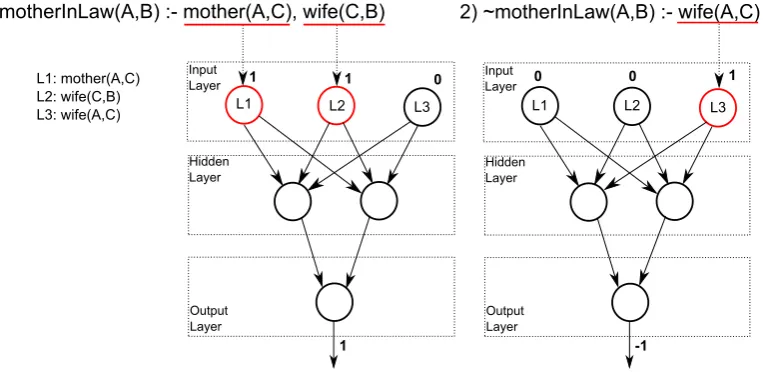
To illustrate the training phase, assume that the bottom clause setE⊥is our training data and no background knowledge has been used. In step 1(a), all body literals from both ex-amples (mother(A,C), wi f e(C,B) andwi f e(A,C)) cause the generation of three new input neurons in the network, with labels identical to the corresponding literals. In step 1(b), an output neuron labeledmotherInLaw(A,B)is added. In step 2, let us assume that two hidden neurons are added. In step 3, zero-weighted connections are added from all three input neu-rons to both hidden neuneu-rons, and from those to the output neuron. Step 4 is only needed when background knowledge is used. In step 5, we add a random non-zero value in[−0.01,0.01]
to each weight. Finally, in step 6, backpropagation is applied (see Fig. 2), firing the input neuronsmother(A,C)andwi f e(C,B)when the positive example is being learned (example 1 in the figure), with target output 1, and firing the input neuronwi f e(A,C)when the negative example is being learned (example 2 in the figure), with target output−1.
Additionally, notice that BCP does not combine first-order literals to generate features like RSD or SINUS: it treats each literal of a bottom clause as a feature. The hidden layer of the ANN can be seen as a (weighted) combination of the features provided by the input layer. Thus, ANNs can combine features when processing the data, which allows CILP++ to group features similarly to RSD or SINUS, but doing so dynamically (during learning), due to the small changes of real-valued weights in the network.
After training, CILP++ can be evaluated. Firstly, each test exampleetestfrom a test setEtest
is propositionalized with BCP, resulting in a propositional data setE⊥test, where eachetest∈Etest
1) motherInLaw(A,B) :- mother(A,C), wife(C,B)
1 1
Input Layer
Hidden Layer
Output Layer
0
1
L1 L2 L3
L1: mother(A,C) L2: wife(C,B) L3: wife(A,C)
2) ~motherInLaw(A,B) :- wife(A,C)
Input Layer
Hidden Layer
Output Layer
0 1
-1 0
[image:15.595.113.495.97.283.2]L1 L2 L3
Figure 2: Illustration of CILP++’s training step. L1, L2 and L3 are labels corresponding to each distinct body literal found inE⊥. The shown output values are the labels which are used for backpropagation training. In the figure, networkNappears repeated for each example, for clarity.
has a corresponding ⊥test
e ∈E⊥test. Then, each ⊥teste is tested in CILP++’s ANN: each input
neuron corresponding to a body literal of ⊥test
e receives input 1 and all other input neurons
(input neurons which labels are not present in ⊥test
e ) receive input 0. Lastly, a feedforward
pass through the network is performed, and the output will be CILP++’s answer to⊥test e and
consequently, toetest.
4
Experimental Results
In this section, we present the experimental methodology and results for CILP++ as a first-order neural-symbolic system and for BCP as a standalone propositionalization method. We also compare results with ILP system Aleph and propositionalization method RSD. Before we experiment on ILP problems, though, we have tested CILP++ against its predecessor, C-IL2P, to evaluate whether CILP++ is as good as C-IL2P on propositional problems. We used the Gene Sequences/Promoter Recognition dataset used in Garcez and Zaverucha (1999) with leave-one-out cross validation. CILP++ obtained 92.41% accuracy, against 92.48% obtained by C-IL2P; CILP++ took 5:21 minutes to run the entire experiment, while C-IL2P took 5:23 minutes. This suggests that CILP++ and C-IL2P perform similarly on propositional problems. As mentioned, we have compared results with Aleph and RSD. Aleph is an ILP system, which has several other algorithms built-in, such as Progol (by default). RSD is a well-known propositionalization method capable of obtaining results comparable to full ILP systems. We have used four benchmarks: the Mutagenesisdataset (Srinivasan and Muggleton, 1994), the
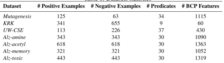
KRK dataset (Bain and Muggleton, 1994), theUW-CSEdataset (Richardson and Domingos, 2006), and the Alzheimers benchmark (King and Srinivasan, 1995), which consists of four datasets: Amine,Acetyl,MemoryandToxic. Table 1 reports some general characteristics and the number of BCP features obtained for each dataset.
Table 1: Datasets statistics
Dataset # Positive Examples # Negative Examples # Predicates # BCP Features
Mutagenesis 125 63 34 1115
KRK 341 655 9 60
UW-CSE 113 226 37 430
Alz-amine 343 343 30 1090
Alz-acetyl 618 618 30 1363
Alz-memory 321 321 30 1052
Alz-toxic 443 443 30 1319
dataset, as explained below), reporting results on six CILP++ configurations. We report: accu-racy vs. runtime on all datasets in comparison with Aleph, and a comparison between BCP and RSD on theMutagenesisandKRKdatasets6. We also evaluate feature selection in CILP++ by constraining the clause length when building bottom clauses with BCP and applying mRMR.
Since a varied number of accuracy results have been reported in the literature on the use of Aleph with theAlzheimersandMutagenesisdatasets (King and Srinivasan, 1995; Landwehr et al., 2007; Paes et al., 2007), we have decided to run both Aleph and CILP++ for our com-parisons. We built 10 folds from each dataset (in the case of UW-CSE, we followed Davis et al. (2005) and used 5 folds) and both systems used the exact same training folds. BCP and RSD could not, however, share the exact same training folds, as a result of the way in which the RSD tool was implemented (the RSD tool generates features before the folds are created, while CILP++ creates the folds in the first place). As mentioned earlier, the CILP++ system, the different configurations/parametrizations, and all the data folds are available for download so that the results reported in this paper should be reproducible. The six CILP++ configurations include:
• st: uses standard backpropagation stopping criteria;
• es: uses early stopping;
• n%bk: the network is created usingn%of the examples inE⊥trainas BK7;
• 2h: uses no building step and starts with 2 hidden neurons only.
The choice of the 2hconfiguration is explained in detail in Haykin (2009); ANNs having two neurons in the hidden layer can generalize binary problems approximately as well as any network. Furthermore, if a network has many features to evaluate, as in the case of BCP, i.e. the input layer has many neurons, it should have sufficient degrees of freedom; further in-creasing it by adding hidden neurons might increase the chances of overfitting. Since bottom clauses are “rough” representations of examples and we would like to model the general char-acteristics of the examples, a simpler model such as 2hshould be preferred (Caruana et al., 2000).
For all experiments with Aleph, the same configurations as in Landwehr et al. (2007) were used for theAlzheimersdatasets (any parameter not specified below used Aleph’s default values): variable depth= 3,least positive coverage of a valid clause= 2,least accuracy of an acceptable clause= 0.7,minimum score of a valid clause= 0.6,maximum number of literals in a valid clause= 5 andmaximum number of negative examples covered by a valid clause (noise)
6Since the available implementation of RSD handles target concepts with arity 1, we were unable to apply the
Alzheimersdatasets to RSD (whose targets have arity 2). An alternative would be to modify the domain knowledge in the datasets, but this is not a straightforward task.
= 300. RegardingMutagenesis, the parameters were based on Paes et al. (2007) (again, if a parameter is not listed below, the Aleph default value has been used): least positive coverage of a valid clause= 4. ForKRK, the configuration provided by Aleph in its documentation was used. ForUW-CSE, the same configuration as in Davis et al. (2005) was used:variable depth= 3,least positive coverage of a valid clause= 10,least accuracy of an acceptable clause= 0.1,
maximum number of literals in a valid clause = 10,maximum number of negative examples covered by a valid clause (noise)= 1000 andevaluation function=m-estimate.
With regards to theUW-CSE dataset, we have used an ILP version of the dataset follow-ing Davis et al. (2005). The original UW-CSE dataset contains positive examples only for use with Markov Logic Networks (Richardson and Domingos, 2006). Davis et. al. gener-ated negative examples for this dataset using Closed World Assumption (Davis et al., 2005). This has produced an unbalanced dataset containing 113 positive examples and 1772 negative examples. Thus, we have re-balanced the dataset by performing random undersampling, un-til we had obtained twice as many negative examples as positive examples. Our goal was to cover the distribution of negative examples as best as possible, while not allowing too much unbalancing, and to provide a fair comparison with Aleph. Alternative undersamplings and oversamplings have been investigated also with results reported below.
As for the CILP++ parameters, we used the same variable depth values as Aleph for BCP (except forUW-CSE, where we usedvariable depth= 1, as discussed below) and the following parameters for backpropagation8: on st configurations, learning rate = 0.1, decay factor = 0.995 and momentum= 0.1; and onesconfigurations: learning rate= 0.05, decay factor= 0.999,momentum= 0 andalpha(early stopping criterion) = 0.01.
Finally, extra hidden neurons were not added to the network configurations above, i.e. step 2 of CILP++’s training algorithm, Section 3.3, was not applied. The networks labeled as2h
have only 2 hidden neurons, and those labeledn%bkhave as many hidden neurons as the size of the BK, i.e.n%the size of the setE⊥train.
4.1 Accuracy Results
In this experiment, CILP++ is evaluated on accuracy vs. runtime against Aleph. Two tables are presented with accuracy averages, standard deviations and complete runtimes over 10-fold cross-validation forMutagenesis, fourAlzheimersdatasets andKRK, and 5-fold cross-validation forUW-CSE, on thest(Table 2) andes(Table 3) CILP++ configurations. By “com-plete runtime” we mean the total building, training and testing times for each system. In both tables, accuracy results in bold are the highest ones and the difference between them and the ones marked with asterisk (*) are statistically significant by two-tailed, paired t-test. All experiments were run on a 3.2 Ghz Intel Core i3-2100 with 4 GB RAM.
Notice how CILP++ can achieve runtimes that are considerably faster than Aleph. We believe the speed-ups are caused by the following main factors: ILP covering-based search al-gorithms have well-known efficiency bottlenecks (Paes et al., 2007, 2008; DiMaio and Shav-lik, 2004), while bottom clause generation is fast, and standard backpropagation learning is efficient (Rumelhart et al., 1986). Further, propositionalized examples are generally easier to handle computationally than first-order examples (Krogel et al., 2003). Tables 2 and 3 for the
st andesconfigurations, respectively, seem to confirm an expected trade-off between speed
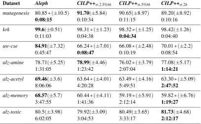
Table 2: Test set accuracy (standard deviation) results and runtimes (in % for accuracy and in hh:mm:ssformat for runtimes) for st configurations. It can be seen that Aleph and CILP++ present comparable accuracy results for the standard CILP++ configurations, with the
st,2.5%bkmodel winning on three datasets. CILP++ performs faster in most cases, confirming our expectation that relational learning through propositionalization should trade accuracy for efficiency, in comparison with full first-order ILP learners.
Dataset Aleph CILP++st,2.5%bk CILP++st,5%bk CILP++st,2h
mutagenesis 80.85∗(±10.5) 91.70(±5.84) 90.65(±8.97) 89.20(±8.92)
0:08:15 0:10:34 0:11:15 0:10:16
krk 99.6(±0.51) 98.31∗(±1.23) 98.32∗(±1.25) 98.42(±1.26)
0:11:03 0:04:38 0:04:34 0:04:40
uw-cse 84.91(±7.32) 66.24∗(±7.01) 66.08∗(±2.48) 70.01∗(±2.2)
0:45:47 0:08:47 0:10:19 0:08:54
alz-amine 78.71(±5.25) 78.99(±4.46) 76.02∗(±3.79) 77.08(±5.17)
1:31:05 1:23:42 2:07:04 1:14:21
alz-acetyl 69.46(±3.6) 63.64∗(±4.01) 63.49∗(±4.16) 63.30∗(±5.09)
8:06:06 4:20:28 5:49:51 2:47:52
alz-memory 68.57(±5.7) 60.44∗(±4.11) 59.19∗(±5.91) 59.82∗(±6.76)
3:47:55 1:41:36 2:12:14 1:19:27
alz-toxic 80.5(±3.98) 79.92(±3.09) 80.49(±3.65) 81.73(±4.68)
6:02:05 3:04:53 3:33:17 2:12:17
and accuracy between propositionalization and methods dealing directly with first-order logic. We can also see thatstconfigurations seem to emphasize accuracy, whileesemphasizes speed. Regarding the CILP++ results onUW-CSE, as mentioned earlier, we have usedvariable depth= 1 for BCP. The reason is thatUW-CSE examples when propositionalized by BCP for
variable depthshigher than 1 become considerably large. At the same time,variable depth
1 causes serious information loss in the propositionalization procedure. To ameliorate this, we have tried an oversampling method called SMOTE, based on kNN (Chawla et al., 2002). SMOTE suggests a combination with random undersampling for better results, whereby we increased the positive examples five times (from 113 to 565 examples) using SMOTE, and undersampled the class of negative examples until we had the same number (565) of negative examples. The problem with this approach, in what concerns a comparison with Aleph, is that, to the best of our knowledge, no oversampling method exists for Aleph; SMOTE is applicable to numerical or propositional data only, thus we could not compare those results with Aleph. Hence, we do not report those results in the accuracy tables above. Nevertheless, with SMOTE, CILP++ obtained 93.34%, 90.11% and 93.58% accuracy for thees,2h,es,2.5%bkandes,5%bk
configurations, respectively. None of the networks took longer than 6 minutes to run (train and test) on all 5UW-CSE folds, including the SMOTE and undersampling pre-processing. Inst
configurations, CILP++ obtained 73.44% for st,2.5%bk, 77.35% forst,5%bk and 74.2% for
Table 3: Test set accuracy (standard deviation) results and runtimes for the CILP++ configu-rations with early stopping (in % for accuracy and in hh:mm:ssformat for runtimes). Using
esmodels, CILP++ was much faster than Aleph but with a considerable decrease in accuracy. Aleph won in accuracy in all but the Mutagenesis dataset. This indicates that early stopping is not recommended in general for use with BCP, unless speed is paramount.
Dataset Aleph CILP++es,2.5%bk CILP++es,5%bk CILP++es,2h
mutagenesis 80.85(±10.51) 83.48(±7.68) 83.01(±10.71) 84.76(±8.34)
0:08:15 0:01:25 0:01:43 0:01:50
krk 99.6(±0.51) 98.16∗(±0.83) 96.33∗(±4.95) 98.31(±1.23)
0:11:03 0:04:08 0:04:28 0:04:18
uw-cse 84.91(±7.32) 68.16∗(±4.77) 65.69∗(±1.81) 67.86∗(±1.79)
0:45:47 0:04:08 0:04:16 0:04:08
alz-amine 78.71(±3.51) 65.33∗(±9.32) 65.44∗(±5.58) 70.26∗(±7.1)
1:31:05 0:35:27 0:08:30 0:10:14
alz-acetyl 69.46(±3.6) 64.97∗(±5.81) 64.88∗(±4.64) 65.47∗(±2.43)
8:06:06 3:04:47 2:42:31 0:25:43
alz-memory 68.57(±5.7) 53.43∗(±5.64) 54.84∗(±6.01) 51.57∗(±5.36)
3:47:55 1:40:51 3:57:39 1:33:35
alz-toxic 80.5(±4.83) 67.55∗(±6.36) 67.26∗(±7.5) 74.48∗(±5.62)
6:02:05 0:12:33 0:14:04 0:28:39
So far, we have explored a number of CILP++ configurations. The use of other config-urations and their combination through tuning sets is possible. However, the ILP literature on Aleph generally reports a single optimal configuration per dataset (and not per fold) (Paes et al., 2007; Landwehr et al., 2007). We believe, therefore, that applying tuning sets to CILP++ would lead to an unfair advantage to the network model, for the sake of comparison with Aleph. Nevertheless, an optimal CILP++ configuration would use tuning sets, and we report those results below on Table 4. A three-fold internal cross validation was applied on the train-ing set of each one of the 10 folds used in Tables 2 and 3. The fold accuracy of the best model, chosen with tuning sets, was then chosen for that fold. Thus, the dataset accuracy of CILP++ using tuning sets is the average of the test set accuracy obtained for each fold with the model that obtained the best tuning set accuracy. We also report the runtimes obtained with this ap-proach and the “best” model for each dataset, which is the one that is chosen the most times, for all the folds. Thebest modelresults shown in the table were used to guide our choice of model in the experiments on feature selection and BCP to follow.
Table 4: Results using tuning sets for CILP++. We report three results in this table, from left to right: CILP++ test set accuracy using tuning sets averaged over the six CILP++ configurations, CILP++ runtime using tuning sets, and best model, i.e. the configuration with most wins on the 10 train/test folds (5 train/test folds, in the case ofUW-CSE). Overall, the beststmodel is thest,2.5%bkconfiguration, the bestesmodel is thees,2hmodel, and the best model overall is thest,2.5%bkmodel.
Dataset Test Set Accuracy Runtime Best model
mutagenesis 88.84(±10.48) 0:07:54 st,5%bk(3/10)
krk 96.75(±4.9) 0:04:19 st,2h(8/10)
uw-cse 66.84(±7.32) 0:06:11 st,2.5%bk(2/5)
alz-amine 76.45(±3.45) 1:31:11 st,2.5%bk(6/10)
alz-acetyl 64.07(±6.2) 0:30:35 es,2h(7/10)
alz-memory 59.67(±5.7) 1:51:02 st,2.5%bk(4/10)
alz-toxic 81.73(±4.68) 2:12:17 st,2h(10/10)
4.2 Comparative Results with Propositionalization
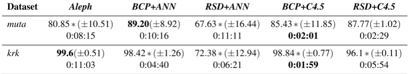
In this section, comparative results against RSD are carried out, using the datasets Muta-genesis (namedmutain the table below) and KRK (the reason for this choice of datasets is explained in the previous section). In Table 5, accuracy and runtimes are shown. We com-pare both BCP and RSD propositionalization when generating training patterns for CILP++ (labeledANNin the table) and for the C4.5 decision tree learner. Aleph results are shown as well as a baseline. We use the CILP++ configuration that obtained the best results in the tun-ing sets for each dataset. Values in bold are the highest obtained, and the difference between those and the ones marked with (*) are statistically significant by two-tailed, unpaired t-test (we use unpaired t-test because of the RSD tool implementation issue, mentioned earlier). All experiments were also run on a 3.2 Ghz Intel Core i3-2100 with 4 GB RAM.
Table 5: Accuracy and runtime results forMutagenesisandKRK datasets (in % for accuracy and in hh:mm:ssformat for runtimes). The results show that BCP is faster than RSD, while showing highly competitive results w.r.t. Aleph, but RSD performed as well as BCP when using C4.5 as learner. BCP outperformed RSD in all models: BCP was faster in all cases, but in theKRK dataset, RSD with C4.5 showed higher accuracy, although the difference was not statistically significant. The results also show that BCP performs well with both learners (ANN and C4.5), but excels with ANNs. On the other hand, RSD did not perform well with ANNs.
Dataset Aleph BCP+ANN RSD+ANN BCP+C4.5 RSD+C4.5
muta 80.85∗(±10.51) 89.20(±8.92) 67.63∗(±16.44) 85.43∗(±11.85) 87.77(±1.02)
0:08:15 0:10:16 0:11:11 0:02:01 0:02:29
krk 99.6(±0.51) 98.42∗(±1.26) 72.38∗(±12.94) 98.84∗(±0.77) 96.1∗(±0.11)
0:11:03 0:04:40 0:06:21 0:01:59 0:05:54
[image:20.595.94.503.608.682.2]empirically confirming our hypothesis.
4.3 Results with Feature Selection
In Section 2.4, it was discussed that, due to the extensive size of bottom clauses, feature selection techniques may obtain improved results when applied after BCP. Two ways of per-forming feature selection were discussed: changing the variable depth (see Algorithm 1) and using a statistical method, mRMR. We have chosen two datasets on which to run these exper-iments with feature selection: Alz-amineandAlz-toxic. We opted for those because CILP++ performed well on them, not outstandingly well (as inMutagenesis), neither poorly (as in Alz-acetyl). Additionally, we have chosen the best stconfiguration (st,2.5bk, chosen by tuning sets) and the best esconfiguration (es,2h). Even though the results using tuning set showed
st,2has the best model for theAlz-toxicdataset, we wanted to analyze feature selection ones
configurations as well, and so we have chosen the bestesconfiguration.
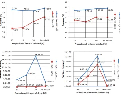
First, we changed the variable depth inAlz-amineandAlz-toxic, which was 3, to 2 and 5, to analyze how changes in this parameter would affect performance. The results are shown in Fig. 3. Alternatively, we applied mRMR with three levels of selection: 50%, 25% and 10% of the best-ranked features. These results are shown in Fig.4.
In summary, statistical feature selection seems to be useful with BCP. Changes in variable depth did not seem to offer gains, but mRMR offered more than 90% feature reduction with a loss of less than 2% in accuracy. The goal of selecting features with mRMR should not be to improve efficiency, although in one case (Alz-amine es-2h), CILP++ with mRMR was faster at 90% feature reduction than CILP++, despite a loss of more than 10% of accuracy.
5
Conclusion and Future Work
This paper has introduced a fast method and algorithm for ILP learning with ANNs, by extending a neural-symbolic system called C-IL2P. The paper’s two contributions are: a novel propositionalization method, BCP, and the CILP++ system, an open-source, freely distributed neural-symbolic system for relational learning. CILP++ obtained accuracy comparable to Aleph on most standard configurations and stood behind Aleph, but was faster, on early stop-ping configurations. In comparison with RSD, CILP++ has been shown superior, but BCP and RSD present similar results when using C4.5 as learner. Nevertheless, BCP obtained better runtime results overall. Lastly, when using feature selection, results have shown that mRMR is applicable with CILP++ and it can reduce drastically the number of features with a small loss of accuracy, despite an increase in runtime in some cases. Feature selection with mRMR can be useful to reduce the size of the network and improve readability, especially if knowledge extraction is needed. Propositionalization methods usually show a trade-off between accuracy and efficiency. Our results show that CILP++ can improve on this trade-off by offering con-siderable speed-up in exchange for small accuracy loss in some datasets, even achieving better accuracy in some cases.
Figure 3: Accuracy (above) with varying variable depth on Alz-amine (left) and Alz-toxic
(right), with runtimes (below) inhh:mm:ssformat. The results indicate that the default vari-able depth is satisfactory: neither increasing it nor decreasing it has helped increase perfor-mance. As stated in Section 2.1, variable depth controls how far the bottom clause generation algorithm goes when generating concept chaining and it is a way of controlling how much in-formation loss the propositionalization method will have. From this and the obtained results, it should be intuitive that higher variable depths should mean a better performance, but together with useful features, it seems to bring redundancy as well.
Figure 4: Accuracy (above) when using mRMR on Alz-amine (left) and Alz-toxic (right), with runtimes (below) inhh:mm:ssformat. The results show that in bothAlz-amineand Alz-toxic datasets, a reduction of 90% in the number of features caused a loss of less than 2% in accuracy, albeit with an increase in runtime. The reduction in features caused CILP++ to take more training epochs to converge and mRMR itself also contributed to the increase in runtime. However, at 90% filtered features, the runtimes approached in general the ones obtained without mRMR filtering. Even with an increase in runtime, feature selection with mRMR seems useful to reduce the size of the network and improve readability, especially if knowledge extraction is to be carried out.
meta-parameters can be useful to CILP++. Furthermore, experiments on datasets with con-tinuous data could be done: it should be interesting to see how CILP++ behaves on this kind of data and to analyze if this approach inherits the additive noise robustness from traditional backpropagation ANNs (Copelli et al., 1997). Also, due to the results for feature selection with mRMR, it is worth evaluating how our approach deals with very large relational datasets, e.g. CORA or Proteins, which are considered to be challenging for ILP learners (Perlich and Merugu, 2005).
References
Bain, M., & Muggleton, S. (1994). Learning optimal chess strategies.Machine Intelligence, 13, 291–309.
Basilio, R., Zaverucha, G., and Barbosa, V. (2001). Learning logic programs with neural net-works. InProc. ILP,LNAI2157: 402–408. Springer.
Caruana, R., Lawrence, S., & Giles, C. L. (2000). Overfitting in neural nets: backpropagation, conjugate gradient, and early stopping. InProc. NIPS, 13: 402–408. MIT Press.
Chawla, N. V., Bowyer, K. W., Hall, L. O., & Kegelmeyer, W. P. (2002). SMOTE: synthetic minority over-sampling technique.Journal of Artificial Intelligence Research, 16 (1): 321– 357.
Clark, P., & Niblett, T. 1989. The CN2 induction algorithm.Machine Learning, 3: 261–283.
Copelli, M., Eichhorn, R., Kinouchi, O., Biehl, M., Simonetti, R., Riegler, P., & Caticha, N. (1997). Noise robustness in multilayer neural networks.EPL (Europhysics Letters), 37 (6): 427–432.
Craven, M., & Shavlik, J. W. (1995). Extracting tree-structured representations of trained net-works. InProc. NIPS, 9: 24–30. Cambridge, MA, USA: The MIT Press.
Davis, J., Burnside, E. S., Dutra, I. C., Page, D., & Costa, V. S. (2005). An integrated ap-proach to learning Bayesian networks of rules. InProc. ECML,LNAI3720: 84–95. Berlin-Heidelberg, Germany: Springer.
De Raedt, L. (2008).Logical and relational learning. Berlin-Heidelberg, Germany: Springer.
De Raedt, L., Frasconi, P., Kersting, K., & Muggleton, S. (2008).Probabilistic inductive logic programming. LNAI 4911. Berlin-Heidelberg, Germany: Springer.
DiMaio, F., & Shavlik, J. W. (2004). Learning an approximation to inductive logic program-ming clause evaluation. InProc. ILP,LNAI3194: 80–97. Springer.
Ding, C., & Peng, H. (2005). Minimum redundancy feature selection from microarray gene expression data.Journal of Bioinformatics and Computational Biology, 3 (2): 185–205.
Džeroski, S., & Lavraˇc, N. (2001). Relational data mining. Berlin-Heidelberg, Germany: Springer.
Garcez, A. S. D., & Zaverucha, G. (2012). Multi-instance learning using recurrent neural networks. InProc. IJCNN. 1–6. IEEE.
Garcez, A. S. D., & Zaverucha, G. (1999). The connectionist inductive learning and logic programming system.Appllied Intelligence, 11: 59–77.
Garcez, A. S. D., Broda, K., & Gabbay, D. M. (2001). Symbolic knowledge extraction from trained neural networks: a sound approach.Artificial Intelligence, 125 (1-2): 155–207.
Garcez, A. S. D., Broda, K. B., & Gabbay, D. M. (2002).Neural-symbolic learning systems. Berlin-Heidelberg, Germany: Springer.
Getoor, L., & Taskar, B. (2007). Introduction to statistical relational learning. Cambridge, MA, USA: The MIT Press.
Guillame-Bert, M., Broda, K., & Garcez, A. S. D. (2010). First-order logic learning in artificial neural networks. InProc. IJCNN. 1–8. IEEE.
Guyon, I., & Elisseeff, A. (2003). An introduction to variable and feature selection.Journal of Machine Learning Research, 3: 1157–1182.
Haykin, S. S. (2009).Neural networks and learning machines. Upper Saddle River, NJ, USA: Prentice Hall.
Jacobs, R. A. (1988). Increased rates of convergence through learning rate adaptation.Neural Networks, 1 (4): 295–307.
Kijsirikul, B., & Lerdlamnaochai, B. K. (2005). First-order logical neural networks. Interna-tional Journal of Hybrid Intelligent Systems, 2 (4): 253–267.
King, R. D., & Srinivasan, A. (1995). Relating chemical activity to structure: An examination of ILP successes.New Generation Computing, 13 (3-4): 411–434.
King, R. D., Whelan, K. E., Jones, F. M., Reiser, F. G. K., Bryant, C. H., Muggleton, S. H., Kell, D. B., & Oliver, S. G. (2004). Functional genomic hypothesis generation and experi-mentation by a robot scientist.Nature, 427 (6971): 247–252.
Koller, D., & Friedman, N. (2009).Probabilistic graphical models: principles and techniques. Cambridge, MA, USA: The MIT Press.
Kramer, S., Lavraˇc, N., & Flach, P. (2001). Propositionalization approaches to relational data mining. In S. Džeroski (Ed.), Relational Data Mining (pp. 262–291). New York, NY, USA: Springer.
Krogel, M. A., Rawles, S., Železný, F., Flach, P., Lavraˇc, N., & Wrobel, S. (2003). Compar-ative evaluation of approaches to propositionalization. InProc. ILP,LNAI2835: 197–214. Springer.
Krogel, M. A., & Wrobel, S. (2003). Facets of aggregation approaches to propositionalization, InProc. ILP,LNAI2835: 30–39. Springer.
Kuželka, O., & Železný, F. (2011). Block-wise construction of tree-like relational features with monotone reducibility and redundancy.Machine Learning, 83: 163–192.
Landwehr, N., Kersting, K., & De Raedt, L. D. (2007). Integrating naive Bayes and FOIL.
Journal of Machine Learning Research, 8: 481–507.
Lavraˇc, N., & Džeroski, S. (1994).Inductive logic programming: techniques and applications. Chichester, UK: E. Horwood.
Møller, M. F. (1993). A scaled conjugate gradient algorithm for fast supervised learning. Neu-ral Networks, 6 (4): 525–533.
Muggleton, S. (1995). Inverse entailment and Progol.New Generation Computing, 13 (3-4): 245–286.
Muggleton, S., & De Raedt, L. D. (1994). Inductive logic programming: theory and methods.
Journal of Logic Programming, 19/20: 629–679.
Muggleton, S., Paes, A., Costa, V. S., & Zaverucha, G. (2010). Chess revision: Acquiring the rules of chess variants through FOL theory revision from examples. InProc. ILP,LNAI
5989: 123–130. Springer.
Muggleton, S., & Tamaddoni-Nezhad, A. (2008). QG/GA: a stochastic search for Progol.
Machine Learning, 70: 121–133.
Nienhuys-Cheng, S. H., & de Wolf, R. (1997).Foundations of inductive logic programming. LNAI 1228. Berlin-Heidelberg, Germany: Springer.
Paes, A., Revoredo, K., Zaverucha, G., & Costa, V. S. (2005). Probabilistic first-order theory revision from examples. InProc. ILP,LNAI3625: 295–311. Springer.
Paes, A., Zaverucha, G., & Costa, V. S. (2008). Revising first-order logic theories from exam-ples through stochastic local search. InProc. ILP,LNAI4894: 200–210. Springer.
Paes, A., Železný, F., Zaverucha, G., Page, D., & Srinivasan, A. (2007). ILP through propo-sitionalization and stochastic k-term DNF learning. InProc. ILP, LNAI 4455: 379–393. Springer.
Perlich, C., & Merugu, S. (2005). Gene classification: issues and challenges for relational learning. InProc. 4th International Workshop on Multi-Relational Mining, ACM. 61–67.
Pitangui, C. G., & Zaverucha, G. (2012). Learning theories using estimation distribution algo-rithms and (reduced) bottom clauses. InProc. ILP,LNAI7207: 286–301. Springer.
Prechelt, L. (1997). Early stopping - but when? InNeural networks: tricks of the trade,LNAI
1524 (2): 55–69. Springer.
Quinlan, J. R. (1993).C4.5: programs for machine learning. San Francisco, CA, USA: Mor-gan Kaufmann.
Richardson, M., & Domingos, P. (2006). Markov logic networks.Machine Learning, 62: 107– 136.
Rumelhart, D. E., Hinton, G. E., & Williams, R. J. (1986). Learning internal representations by error propagation. In D. E. Rumelhart, & J. L. McClelland (Eds.), Parallel distributed processing: explorations in the microstructure of cognition(pp. 318–362). Cambridge, MA, USA: MIT Press.
Rumelhart, D. E., Widrow, B., & Lehr, M. A. (1994). The basic ideas in neural networks.
Communications of the ACM, 37 (3): 87–92.
Srinivasan, A., & Muggleton, S. H. (1994). Mutagenesis: ILP experiments in a non-determinate biological domain. InProc. ILP,LNAI237: 217–232.
Tamaddoni-Nezhad, A., & Muggleton, S. (2009). The lattice structure and refinement op-erators for the hypothesis space bounded by a bottom clause.Machine Learning, 76 (1): 37–72.
Uwents, W., Monfardini, G., Blockeel, H., Gori, M., & Scarselli, F. (2011). Neural networks for relational learning: an experimental comparison.Machine Learning, 82 (3): 315–349.