A Multi-temporal fusion-based approach for land cover mapping in support of nuclear incident response

Rochester Institute of Technology

RIT Scholar Works

Theses Thesis/Dissertation Collections

1-28-2013

A Multi-temporal fusion-based approach for land

cover mapping in support of nuclear incident

response

Follow this and additional works at:http://scholarworks.rit.edu/theses

This Thesis is brought to you for free and open access by the Thesis/Dissertation Collections at RIT Scholar Works. It has been accepted for inclusion in Theses by an authorized administrator of RIT Scholar Works. For more information, please [email protected].

Recommended Citation

A MULTI-TEMPORAL FUSION-BASED APPROACH FOR LAND COVER

MAPPING IN SUPPORT OF NUCLEAR INCIDENT RESPONSE

by

Shagan Sah

Bachelor of Engineering,

Pune University, 2009

A thesis submitted in partial fulfillment of the requirements for the degree of Master of Science in the Chester F. Carlson Center for Imaging Science

of the College of Science Rochester Institute of Technology

January 28, 2013

Signature of the Author

Accepted by

CHESTER F. CARLSON CENTER FOR IMAGING SCIENCE

COLLEGE OF SCIENCE

ROCHESTER INSTITUTE OF TECHNOLOGY

ROCHESTER, NEW YORK

CERTIFICATE OF APPROVAL

M.S. DEGREE THESIS

The M.S. Degree Thesis of Shagan Sah has been examined and approved by the thesis committee as satisfactory for the

thesis requirement for the M. S. degree in Imaging Science

Dr. Jan van Aardt, Thesis Advisor

Dr. David Messinger, Committee

Dr. Anthony Vodacek, Committee

Dr. Peter Bajorski, Committee

THESIS RELEASE PERMISSION

CHESTER F. CARLSON CENTER FOR IMAGING SCIENCE

ROCHESTER INSTITUTE OF TECHNOLOGY

Title of Thesis:

A Multi-temporal Fusion-based Approach for Land Cover Mapping in Support of Nuclear Incident Response

I, Shagan Sah, hereby grant permission to the Rochester Institute of Technology to reproduce my print thesis or dissertation in whole or in part. Any reproduction will not be for commercial use or profit.

ABSTRACT

An increasingly important application of remote sensing is to provide decision

support during emergency response and disaster management efforts. Land cover maps

constitute one such useful application product during disaster events; if generated rapidly

after any disaster, such map products can contribute to the efficacy of the response effort.

In light of recent nuclear incidents, e.g., after the earthquake/tsunami in Japan (2011), our

research focuses on constructing rapid and accurate land cover maps of the impacted area

in case of an accidental nuclear release. The methodology involves integration of results

from two different approaches, namely coarse spatial resolution multi-temporal and fine

spatial resolution imagery, to increase classification accuracy. Although advanced

methods have been developed for classification using high spatial or temporal resolution

imagery, only a limited amount of work has been done on fusion of these two remote

sensing approaches.

The presented methodology thus involves integration of classification results from

two different remote sensing modalities in order to improve classification accuracy. The

data used included RapidEye and MODIS scenes over the Nine Mile Point Nuclear

Power Station in Oswego (New York, USA). The first step in the process was the

construction of land cover maps from freely available, high temporal resolution, low

spatial resolution MODIS imagery using a time-series approach. We used the variability

in the temporal signatures among different land cover classes for classification. The time

series-specific features were defined by various physical properties of a pixel, such as

variation in vegetation cover and water content over time. The pixels were classified into

Mahalanobis distance metrics. On the other hand, a high spatial resolution commercial

satellite, such as RapidEye, can be tasked to capture images over the affected area in the

case of a nuclear event. This imagery served as a second source of data to augment

results from the time series approach. The classifications from the two approaches were

integrated using an a posteriori probability-based fusion approach. This was done by

establishing a relationship between the classes, obtained after classification of the two

data sources. Despite the coarse spatial resolution of MODIS pixels, acceptable

accuracies were obtained using time series features. The overall accuracies using the

fusion-based approach were in the neighborhood of 80%, when compared with GIS data

sets from New York State. This fusion thus contributed to classification accuracy

refinement, with a few additional advantages, such as correction for cloud cover and

providing for an approach that is robust against point-in-time seasonal anomalies, due to

the inclusion of multi-temporal data.

We concluded that this approach is capable of generating land cover maps of

acceptable accuracy and rapid turnaround, which in turn can yield reliable estimates of

crop acreage of a region. The final algorithm is part of an automated software tool, which

can be used by emergency response personnel to generate a nuclear ingestion pathway

Acknowledgements

I would like to thank all the professors, staff, and all my fellow students at the

Imaging Science department at RIT, for the wonderful experience and knowledge I have

received throughout the program. I am deeply indebted to Dr. Jan van Aardt, my teacher

and advisor, for providing his valuable time and guidance throughout the research

process and writing of this thesis. His constant encouragement and support towards

experimenting with new ideas really had me going. I am greatly honored to have worked

under him.

I would like to thank the members of my advisory committee, Dr. David

Messinger, Dr. Anthony Vodacek, and Dr. Peter Bajorski, for providing their knowledge

and expertise throughout this project. I would also like to thank Mr. Don Mckeown for

his help during the initial phase of this research. My gratitude goes out to Cindy Schultz,

for her encouragement and support during my time with the DIRS group. This thesis

would not have been possible without help and support of all the people around me, who

were always kind and willing to give their time and valuable assistance towards the

completion of this thesis. Finally, my sincere thanks goes to the Chester F. Carson Center

for Imaging Science at RIT and the National Science Foundation for providing financial

support in the development of this thesis.

My deepest gratitude goes to my family for their support throughout this graduate

Table of Contents

Chapter 1 Introduction ...1

1.1. Multispectral Classification ... 6

1.2. Temporal Classification ... 9

1.3. Fusion-based Classification ... 15

1.4. Hypothesis and Objectives ... 19

Chapter 2 Methodology ...20

2.1. Study Area ... 22

2.2. Imagery Specifications ... 24

2.3. Data Preprocessing ... 24

2.4. Time Series Classification ... 26

2.4.1 Time Series Feature Metric Extraction ... 35

2.4.2 Classification Metrics ... 37

2.5. High Spatial Resolution Classification (RapidEye) ... 39

2.6. The Fusion Method ... 40

2.7. Error Analysis ... 41

Chapter 3 Results and Discussion ...43

3.1. Time Series Classification ... 43

3.3. Fusion Results... 57

Chapter 4 Conclusion ...63

Bibliography ...67

Appendix A - Algorithms ...74

A.1 RapidEye data processing ... 74

A.2 Time-series processing ... 79

List of Figures

FIGURE 1.1AN EXAMPLE OF A NUCLEAR INGESTION PATHWAY FROM THE NINE MILE POINT NUCLEAR

POWER PLANT,OSWEGO,NY, WHICH SHOWS THE AREA EFFECTED BY A HYPOTHETICAL NUCLEAR

FALLOUT. ... 3

FIGURE 1.2LAND USE MAP FROM USGS AROUND THE NINE MILE POINT NUCLEAR POWER PLANT.IN THE

RADIUS OF 10 KM AROUND THE PLANT, THERE ARE APPROXIMATELY 3600 HECTARES OF

AGRICULTURAL LANDS. ...10

FIGURE 1.3FLOWCHART FOR THE FIRST FUSION STRATEGY, WHICH COMBINES LAYERS OF IMAGES OF

VARYING RESOLUTION AND THEN CLASSIFIES THEM (CHEN AND STOW,2003). ...17

FIGURE 1.4FLOWCHART FOR THE SECOND STRATEGY ON COMBINATION OF VARIOUS SPATIAL RESOLUTIONS

(CHEN AND STOW,2003).THIS IS A BOTTOM-UP APPROACH WHERE PIXELS ARE ASSIGNED TO THE

CLASS WITH HIGHEST POSTERIORI PROBABILITY AT EACH RESOLUTION. ...17

FIGURE 1.5FLOWCHART FOR THE THIRD STRATEGY FROM (CHEN AND STOW,2003), WHICH INVOLVES A TOP

-DOWN APPROACH FOR FUSION OF CLASSIFICATION MAPS. ...18

FIGURE 2.1.BLOCK DIAGRAM OF THE ENTIRE ALGORITHM WORKFLOW, BASED ON COARSE RESOLUTION (CR)

MULTI-TEMPORAL MODIS AND HIGH SPATIAL RESOLUTION (HR)RAPIDEYE IMAGERY. ...21

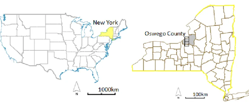
FIGURE 2.2STUDY AREA -OSWEGO COUNTY,NEW YORK,USA, SHOWING THE RAPIDEYE IMAGE GRIDS. ...23

FIGURE 2.3REPRESENTATION OF A "TEMPORAL STACK" OF MODIS IMAGERY, WHERE THE TEMPORAL

DIMENSION FOR A PIXEL AT A SPECIFIC WAVELENGTH OR INDEX IS REPRESENTED IN THE THIRD

DIMENSION. ...29

FIGURE 2.4AN EXAMPLE OF A MODIS“HYPER-TEMPORAL” RED REFLECTANCE CURVE (SHOWN FOR THE

PIXEL INDICATED ON THE LEFT RGB IMAGE).THE THIRD DIMENSION OR THE BAND NUMBER

REPRESENTS A TIME PERIOD OF FIVE YEARS WITH A 16-DAY RESOLUTION. ...29

FIGURE 2.5AN EXAMPLE OF A RAPIDEYE SCENE MARKED WITH MODIS PIXEL SIZE BLOCKS.MIXTURE OF

DIFFERENT LAND CLASSES CAN BE OBSERVED IN MODIS PIXELS. ...30

FIGURE 2.6SMOOTHED NORMALIZED DIFFERENCE VEGETATION INDEX (NDVI) TEMPORAL PROFILES FOR

FIGURE 2.7SMOOTHED ENHANCED VEGETATION INDEX (EVI) TEMPORAL PROFILES FOR THE FOUR CLASSES.

...33

FIGURE 2.8SMOOTHED SOIL ADJUSTED VEGETATION INDEX (SAVI) TEMPORAL PROFILES FOR THE FOUR

CLASSES. ...34

FIGURE 2.9SMOOTHED MODIFIED SOIL ADJUSTED VEGETATION INDEX -2(MSAVI-2) TEMPORAL PROFILES

FOR THE FOUR CLASSES...34

FIGURE 2.10EVI TIME SERIES CURVES FOR FOUR LAND COVER CLASSES AFTER SAVITZKY-GOLAY

SMOOTHING.A NUMBER OF DISTINCT FEATURES WERE OBSERVED, E.G., PEAK-TO-PEAK VALUES FOR

THE FOREST CLASS WAS HIGH, WHILE URBAN AND VEGETATION CLASSES HAVE REDUCED VALUES AT

TROUGHS, WHICH WAS ATTRIBUTED TO BARE SOIL EXPOSURE IN WINTER. ...36

FIGURE 3.1AN EVI TIME SERIES FOR A TYPICAL VEGETATION COVER PIXEL, BEFORE AND AFTER THE

SAVITZKY-GOLAY SMOOTHING, TO FILTER HIGH FREQUENCY SPIKES. ...44

FIGURE 3.2ILLUSTRATION OF MODIS OUTPUT SCALE.(A)AN EXAMPLE MODIS(250 M) CLASS MAP FOR

FOUR CLASSES DERIVED USING MAHALANOBIS DISTANCE CLASSIFICATION;(B) A HIGH RESOLUTION

RGB IMAGE (5 M) FROM RAPIDEYE OVER THE SAME AREA FOR COMPARISON. ...48

FIGURE 3.3RAPIDEYE SAMPLE SHOWING CLOUD COVERED LAND AREAS (LEFT) AND RESULTS FROM THE

CLOUD MASKING ALGORITHM, BASED ON A RED BAND THRESHOLD (RIGHT). ...51

FIGURE 3.4EXAMPLE OF SPECTRAL BEHAVIOR SIMILARITY BETWEEN THE FOREST AND AGRICULTURE CLASS

FOR RAPIDEYE BANDS. ...52

FIGURE 3.5A SAMPLE RAPIDEYE SCENE AND CORRESPONDING CLASS MAP, BASED ON THE EUCLIDEAN

DISTANCE CLASSIFICATION. ...53

FIGURE 3.6A SAMPLE RAPIDEYE SCENE AND CORRESPONDING CLASS MAP, BASED ON THE MAHALANOBIS

DISTANCE CLASSIFICATION. ...54

FIGURE 3.7ARAPIDEYE CLASSIFICATION MAP THAT DEMONSTRATES THE DISADVANTAGES OF USING A

SINGLE-DATE IMAGE FOR CLASSIFICATION...56

FIGURE 3.8SPECTRAL REFLECTANCE COMPARISON FOR URBAN CLASS WITH A CROP SITE AT INITIAL GROWTH

FIGURE 3.9CLASS MAPS FOR,(A) COARSE SPATIAL RESOLUTION (CR) TIME-SERIES,(B) HIGH SPATIAL

RESOLUTION (HR) MULTI-SPECTRAL, AND (C) FUSION-BASED CLASSIFICATION, USING THE

MAHALANOBIS DISTANCE AS METRIC FOR CLASSIFICATION. ...60

FIGURE 3.10AN ILLUSTRATION OF CLASSIFICATION RESULTS AT 5M SPATIAL RESOLUTION:(A)RAPIDEYE

(5M)RGB IMAGE OF AN AREA WITH CLOUD COVER,(B)RAPIDEYE LAND COVER CLASSIFICATION USING

THE EUCLIDEAN DISTANCE, AND (C) THE CLASSIFICATION RESULT AFTER FUSION OF CLASS MAPS FROM

List of Tables

TABLE 1.1FEW EXAMPLES OF VARIOUS MULTISPECTRAL IMAGE CLASSIFICATION METHODS FROM THE

LITERATURE. ... 7

TABLE 2.1DATA SPECIFICATIONS FOR THE MODIS AND RAPIDEYE IMAGERY. ...24

TABLE 2.2DESCRIPTION OF THE FINAL FOUR LAND COVER TYPES USED IN THE CLASSIFICATION ALGORITHM.

...32

TABLE 2.3TIME SERIES FEATURE METRICS COMPUTED USING THE TEMPORAL PROFILES. ...35

TABLE 3.1A LIST OF THE SUBSET TEMPORAL FEATURE METRICS, AS IDENTIFIED VIA THE STEPWISE

DISCRIMINANT ANALYSIS. ...45

TABLE 3.2CONFUSION MATRIX, OVERALL ACCURACY AND KAPPA STATISTICS FOR TIME SERIES MODIS

CLASSIFICATION USING MAHALANOBIS DISTANCE AS THE CLASSIFICATION METRIC. ...47

TABLE 3.3CONFUSION MATRIX FOR RAPIDEYE HIGH SPATIAL RESOLUTION CLASSIFICATION USING THE

EUCLIDEAN DISTANCE METRIC. ...53

TABLE 3.4CONFUSION MATRIX FOR THE RAPIDEYE HIGH SPATIAL RESOLUTION CLASSIFICATION USING THE

MAHALANOBIS DISTANCE METRIC. ...54

TABLE 3.5CONFUSION MATRIX FOR FUSION-BASED CLASSIFICATION USING THE EUCLIDEAN DISTANCE

METRIC. ...57

TABLE 3.6CONFUSION MATRIX FOR THE FUSION-BASED CLASSIFICATION USING THE MAHALANOBIS

DISTANCE METRIC. ...58

TABLE 3.7CLASSIFICATION ACCURACIES AND KAPPA VALUES FOR THE COARSE SPATIAL RESOLUTION TIME

SERIES, HIGH SPATIAL RESOLUTION MULTI-SPECTRAL, AND FUSION-BASED METHODS.EUCLIDEAN

Chapter 1

Introduction

Remote sensing data providers, scientists, algorithm specialists, and disaster

response agencies often collaborate to develop effective ways to prevent and respond to a

variety of disaster scenarios and provide associated relief measures. Remote sensing and

geographic information systems (GIS) are among many tools available today for disaster

management efforts, which contribute to making many disaster response efforts more

efficient. For example, remote sensing can be used to rapidly generate land cover maps

for assisting emergency response personnel with resource deployment decisions and

impact assessments. But, despite the presence of numerous satellites with varying spatial,

temporal, spectral, and radiometric resolutions, none of them have been solely designed

for the purpose of observing disasters or natural hazards (Nirupama, 2002).

In light of recent disaster events at the Fukushima nuclear power facility in Japan,

caused by the earthquake and associated tsunami of 2011, there has been an increased

awareness of the problem of managing a major radiological release on the part of

emergency response agencies. The accurate mapping of the “ingestion exposure

pathway”, which refers to the area affected by the deposition of radionuclides on crops,

other vegetation (such as pasture and animal feed), bodies of surface water, and ground

surfaces, is among the most critical issues. In other words, a nuclear ingestion pathway or

simply a nuclear plume, is the area surrounding a nuclear facility site (usually with a

radius of approximately 15-20 km) that has been subjected to radioactive exposure (for

resource usage and food ingestion by humans (New York State Radiological Emergency

Planning, 2010). Emergency managers need up-to-date inventories of crops, vegetation,

open water, and drainage features in an affected area to determine the impact of a release.

Information on the acreage, type, and geographic distribution of the affected areas will

drive decision-making relative to the response; this information also provides a

quantitative basis for economic impact assessment.

Remotely sensed imagery, based on aircraft- or satellite-based sensors with

sufficient spatial and spectral resolution, can potentially be used to accurately map and

discriminate crop/ground cover types, open water bodies, and impervious surfaces

(runoff) (Vinciková et al., 2010). This land cover classification is an important remote

sensing or geospatial product and is typically derived based on spatial, spectral, or

temporal characteristics of individual or grouped pixels (Lu and Weng, 2007). The

resultant accurate and timely produced land cover maps can provide essential information

during and after a regional, national, or a global scale disaster. In this study, we focus on

deriving accurate land cover maps to identify the impacted area in the case of an

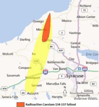
Figure 1.1 An example of a nuclear ingestion pathway from the Nine Mile Point Nuclear Power Plant, Oswego, NY, which shows the area effected by a hypothetical nuclear fallout.

Remote sensing of the ingestion exposure pathway requires imaging a large area

in a timely fashion. The Federal Emergency Management Agency (FEMA), in their

Ingestion Pathway Exercise (2000), reported that an affected area may be tens of

thousands to several hundred thousand hectares. A typical airborne mapping system (one

aircraft and sensor) can cover approximately 200-250 km2 per day (weather permitting)

can be launched at virtually anytime, weather permitting; however, aircraft operations do

need to be mobilized for an event, which may require a day or more of planning and

deployment from wherever the system is based and as stated before, is limited in terms of

aerial coverage. Another significant challenge for aircraft data acquisition is that an

ongoing radiological incident may preclude the safe operation of manned air assets,

especially near the reactor site or for any extended period of time.

High spatial resolution commercial satellites have the potential to rapidly cover

large areas. For example, a satellite can cover hundreds of square kilometers in a single

pass as can be observed from specification of various satellite sensors (Satellite Imaging

Corporation). Satellites are also not restricted by hazards in the affected area. In the case

of a catastrophe, with an increasing number of available high spatial resolution satellites

such as Quickbird, IKONOS, RapidEye, etc., any number of satellites could be tasked to

acquire images of the affected area. Most high spatial resolution imaging satellites are in

a state of continuous readiness and can be tasked within minutes or hours (Gillespie et

al., 2007). However, there are potential limitations due to orbital geometry and weather.

For example, it may be several days before a satellite’s ground track passes over a

particular location or the ground track may not be well aligned with the plume area. High

clouds that would not impact airborne operations, on the other hand, would render

satellite imaging ineffective and result in another waiting period before the next pass.

In addition, land cover classification based on a single image is potentially less

accurate and more challenging to derive, given the occurrence of poor weather

conditions, e.g., cloud cover, or the spatial and spectral limitations of the sensor (Robin et

this research involves the fusion of classification results from two satellite image sources

- a single date, high spatial resolution, multi-spectral image and coarse spatial resolution,

high temporal resolution, freely available imagery over the same area. We used a

RapidEye image for the high spatial resolution multi-spectral classification; the presence

of the red edge band in the RapidEye band set has made this sensor a useful resource for

vegetation-related applications. For example, Tapsall et al. (2010), Kim et al. (2011), and

Sousa et al. (2012) have analyzed the use of RapidEye images for a variety of natural

resource applications. Details of the RapidEye satellite constellation are listed in the

methods section.

Several studies also have been conducted in the past to assess the appropriate

spatial resolution for classification, most notably the work by Atkinson and Curran

(1997). Other authors also found that the best classification results can be achieved for a

specific land cover class by using a particular combination of resolution and algorithm;

however, it is hard to achieve the best results for all classes using just a single

combination of a resolution and an algorithm (Marceau et al., 1994; Ponzoni et al.,

2002). It thus stands to reason that the strategy of integrating class maps at two different

resolutions can be regarded as a necessary component in the process of land cover

mapping. This is underscored by a large number of fusion-based image classification

methods that exist in the literature, all of which use the combination of several sources of

information with the basic aim of augmenting and increasing the reliability of

classification results. The final objective of this research was to augment the

coarse spatial resolution time series imagery. Note: In order to facilitate discussion, the

term “resolution” will be assumed to imply “spatial resolution” from this point forward.

In the following subsections, we will discuss various classification methods from

the literature. For our application, multispectral, time-series, and fusion-based

classification methods are reviewed.

1.1.

Multispectral Classification

Radiance from the Earth’s surface is measured by a variety of satellite sensors and

typically converted to approximate surface reflectance measurements, which in turn are

used to extract information for specific surface targets, i.e., towards application of the

acquired imagery to a specific problem. Image classification and segmentation into land

cover, material, or object classes, are among the most important applications of remote

sensing. Classification of any form of data can be broadly categorized into supervised and

unsupervised approaches. In unsupervised methods, an algorithm is developed to group

pixels with similar characteristics, while supervised approaches rely on a user to identify

a sample of pixels of each class/cover type and use various signal processing algorithms

to assign pixels from the image to class with the highest membership probability (Schott,

2007).

There are a number of algorithms that target the analysis of multispectral data.

The traditional methods for image classification algorithms include K-means and

can easily be applied through widely available image processing or statistical software

packages (Xie et al., 2008). Artificial neural networks and fuzzy logic approaches for

image classification and vegetation applications are also abundant in the literature, but

often lack transparency (Zhang and Foody, 1998; Filipi and Jensen, 2006). Our goal was

not to evaluate different classification approaches, but rather to focus on a novel

multi-temporal, multi-resolution approach based on established classification algorithms. A few

examples of classification algorithms based on multispectral data are listed in Table 1.1. The reader therefore is referred to the in-depth review of various classification methods

by Lu and Weng (2007).

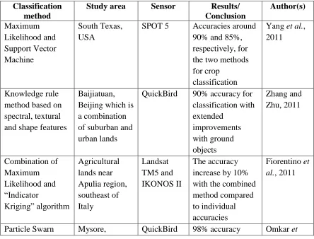
Table 1.1 Few examples of various multispectral image classification methods from the literature.

Classification method

Study area Sensor Results/ Conclusion Author(s) Maximum Likelihood and Support Vector Machine South Texas, USA

SPOT 5 Accuracies around 90% and 85%, respectively, for the two methods for crop

classification

Yang et al., 2011

Knowledge rule method based on spectral, textural and shape features

Baijiatuan, Beijing which is a combination of suburban and urban lands

QuickBird 90% accuracy for classification with extended improvements with ground objects Zhang and Zhu, 2011 Combination of Maximum Likelihood and “Indicator Kriging” algorithm Agricultural lands near Apulia region, southeast of Italy Landsat TM5 and IKONOS II The accuracy increase by 10% with the combined method compared to individual accuracies

Fiorentino et al., 2011

Classification method

Study area Sensor Results/ Conclusion Author(s) Optimization and Ant-Miner algorithm Karnataka, India

when the swarn intelligence used the relation between various input data

al., 2007

Spectral Angle Mapper Clarion, Pennsylvania, US Landsat TM5 Overall accuracy of 93% and the method does not require the data to be normally distributed Sohn and Rebello, 2002 Artificial Neural Network South west Florida Landsat TM 5 Overall accuracy of 78 %, but it depends on the number of hidden units Dixon and Candade, 2008 Object-based classification Phoenix, Arizona

QuickBird Better results than the classical per-pixel classifier, with accuracies of 90%

Myint et al., 2011

We used two different classification techniques, based on spectral and temporal

properties of different pixels, at various stages throughout the algorithm. The first was the

minimum distance or the Euclidean distance classification, which calculates the spectral

distance between the measurement vector for the candidate pixel and the mean vector for

each class or signature. The candidate pixel is assigned to the class with the shortest

distance. The main drawback with the minimum distance method is its inability to

consider class variability/co-linearity. The second method was the Mahalanobis distance

method, which is based on the correlation between the variables. It uses the mean and

from the local class mean. The advantage with Mahalanobis distance method is the

inclusion of class variability using the covariance matrix (Schott, 2007).

The next section reviews relevant published articles on various methods, all of

which use temporal information as input to the classification.

1.2.

Temporal Classification

The second step in the multi-temporal, multi-resolution algorithm involved

construction of a coarse-scale land cover map from freely available, high temporal

resolution data using a time-series approach. Given the fact that most of the landmass

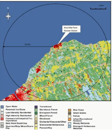
worldwide is covered by vegetation (in particular consider our study area in Figure 1.2), the application of phenological differences through time series analysis of imagery could

yield accurate land cover map (Knight et al., 2006). Such an approach is further

facilitated by improved satellite revisit times (temporal resolution); multi-temporal data

are now available which help to characterize objects based on their dynamic properties, in

Figure 1.2 Land use map from USGS around the Nine Mile Point Nuclear Power Plant. In the radius of 10 km around the plant, there are approximately 3600 hectares of agricultural lands.

Recent studies on land cover classification increasingly have used multi-temporal

remotely sensed data sets, e.g., Boles et al. (2004) achieved accuracies around 70% using

east Asia. They also reported maximum misclassifications among the woody vegetation,

grasslands, sparse vegetation and croplands classes. In another study, Sakamoto et al.

(2005), determined different phenological stages of vegetation growth in terms of time in

days, using maximum, minimum and inflection points from time profiles and obtained

offset errors of approximately 10 days. An important conclusion was the presence of

errors in phenological stages due to mixed pixels effects. Zhang et al. (2008) used a

decision tree analysis on the time-series of MODIS images over North China Plain and

reported a 75% accuracy. Most of these studies have commonly described the vegetation

dynamics based on phenological variations over time. Researchers have exploited typical

satellite vegetation indices, such as Normalized Difference Vegetation Index (NDVI) and

Enhanced Vegetation Index (EVI), which are directly correlated with the green biomass,

and are frequently used for studying land cover dynamics. In this study, time profiles

from a number of spectral bands, along with derived vegetation indices, were used as

temporal input data. Keeping all the requirements and constraints in view, the Moderate

Resolution Imaging Spectro-radiometer (MODIS) time-series data were used for

generating land cover maps at a coarse resolution. We therefore will discuss the methods

and results of some more common methods where MODIS time series imagery was used

for various forms for land cover classification.

The use of temporal signatures of different classes as features for classification is

a common approach while working with time profiles. For example, Gupta and Rajan

(2010), used MODIS data over the Dharwad District in Karnataka, India, and applied

dynamic time warping as a distance measure to form a curve matching scheme; the

classes, namely forest, crop, and water. Similarly, class separability among specific crop

types was investigated using the Jeffries-Matusita distance statistic, using MODIS EVI

and NDVI data over Kansas State in USA (Wardlow et al., 2007). They concluded that

NDVI and EVI exhibited a high correlation when used to describe vegetation cover.

Another very common approach while working with temporal profiles, is the decision

tree method. This was successfully applied by Zhang et al. (2008), by basing the decision

nodes on the values of phenological features derived through time, but their approach was

also dependent on other physical features, such as land surface temperature and surface

slope. The work by Jönsson and Eklundh (2004) also deserves special mention – these

authors developed a widely popular user algorithm and interface dubbed “TIMESAT”.

The interface assists the user in describing the land dynamics by viewing the

phenological variation of MODIS EVI time-series throughout the course of a year.

Finally, among the more mathematically complicated methods, the back-propagation and

fuzzy neural network approach, used for multi-temporal image classification, increased

classification accuracies by 10-15%, when compared with conventional multi-temporal

methods (Kushardono et al., 1995). However, most of these studies produce land cover

maps at a lower resolution that lack definition of high spatial resolution features.

In many of the previous studies, data in the form of vegetation indices from other

satellites were also used for temporal analysis of land cover. For example, ISODATA

classification using data from the SPOT sensor resulted in a maximum accuracy of 80%,

while validating the results using a Landsat-derived land cover data (Boles et al., 2004).

Similarly, Lhermitte et al. (2008) have applied hierarchical segmentation on the fast

sensor to describe the spatio-temporal features to analyze actual vegetation. They

concluded that more multi-scale studies are crucial to get a better relationship between

time-series data and the ecosystem they represent. This approach was also successfully

demonstrated by Wen et al. (2010), who used MODIS EVI time-series over grasslands in

Tibet, and obtained accuracies of approximately 68%. Kandrika and Roy (2008), on the

other hand, evaluated the temporal spectral responses using the IRS-P6 (Resourcesat)

dataset over eastern parts of India to classify land cover. The authors implemented a

decision tree approach and obtained accuracies of 87%. Likewise, numerous other studies

are present in the literature, all of which have used different sensor datasets in a temporal

approach to achieve land cover maps. However, the majority of past studies have

preferred approaches based on MODIS data for time-series analysis, because of a variety

of reasons, e.g., improved atmospheric and cloud screening, consistent data availability,

low cost (free), high temporal resolution (8-day and 16-day) and above all, the vast range

of spectral and data products (Carrão et al., 2008). It should also be noted that most of the

work involving time series data is focused on vegetation applications. Another very

important application of time-series data is change detection, e.g., through filtering the

MODIS NDVI time-series data, to obtain a 89% accuracy in change detection of new

settlements in South Africa (Kleynhans et al., 2011). Lunetta et al. (2006), also

evaluating vegetation spectral time series, achieved change detection accuracies of 88%

while comparing discrete Fourier transformed time-series of MODIS NDVI data over

Albemarle-Pamlico Estuary System in North Carolina. However, the question of which

The issue of data redundancy when working with time series revolves around the

large number of data channels or bands, with the majority of bands containing

superfluous information (Chandola et al., 2010). This could in turn affect the

performance of the classifier, due the Hughes phenomenon (Hsieh and Landgrebe, 1998).

For practical reasons, the computational cost also increases with an increase in the feature

space dimension. Thus, data reduction constitutes an important step when working with

high dimensional time-series data (Carrão et al., 2008). As demonstrated successfully by

Zhang et al. (2008) and Sakamoto et al. (2005), we used temporal attributes extracted

from the time series as features for classification. Feature space data reduction relied on

stepwise discriminant analysis, which has been widely used in the remote sensing

community, e.g., for spectral band selection in hyperspectral images (Hochberg and

Atkinson, 2000; Karimi et al., 2005; van Aardt and Rogers, 2008) or with other forms of

datasets like feature reduction with light detection and ranging (lidar) (van Aardt et al.,

2011). It should also be noted that the selection of a suitable classification method is

application dependent, while also varying with testing and training data and the number

of classes.

The third step in our algorithm was fusion of classification results from a single

multispectral high resolution image and time-series coarse resolution image. The next

1.3.

Fusion-based Classification

Multi-sensor image fusion is among the fundamental tools of image processing

and has gained more traction in land cover classification, mainly because of numerous

limitations (spatial, spectral, or temporal) associated with individual satellite sensors. One

of our objectives for this study was to increase land cover classification accuracy through

image fusion, in contrast to single modality classification approaches. There are a variety

of existing algorithms that focus on fusion of classification information from sensors with

different spatial resolutions. The Bayesian approach for multi-scale land classification

remains popular among fusion studies. For example, Robin et al. (2005) obtained

accuracies >90%, when combining Bayesian theory with a linear mixture model.

However, their approach was limited to images with resolution ratios of 15 and the

method was only demonstrated using simulated images. In another Bayesian theory based

approach, Storvik et al. (2005) used a reference resolution from the SPOT-5 sensor over

downtown Paris to obtain an overall probability of correct classification of 88%. Kumar

et al. (2011), in an enhancement to the Bayesian method, proposed a new technique

which contrasts the most widely used Bayesian classifiers, by not assuming equal prior

probabilities for all classes. Their method increased the land cover classification

accuracies by 6% and 9% with IRS LISS-III MS and IKONOS data, respectively.

However, the method increased the computational requirements and was not suitable for

near-real time applications.

Apart from a Bayesian approach, another notable effort was developed in the

resolution image to generate a classification map at the higher resolution. The authors

used data from the Landsat 5 and MODIS sensors for purposes of training and validation,

respectively. In other studies, neural networks were applied for classification of

multisource datasets. Examples include Bruzzone et al. (1999), who applied Landsat 5

and Synthetic Aperture Radar data into a single layer neural network and obtained errors

<5%, and Liu et al. (2001), who used an Adaptive Resonance Theory neural network on

MODIS and Landsat TM, and predicted 80% of each classes within the 10% error bound.

Yet another context-dependent method, in this case using a two-dimensional Hidden

Markov Model for multi-resolution classification, was successfully demonstrated by Li et

al. (2000). The biggest challenge in all of these multi-resolution approaches was the

multi-to-single date spatial correspondence between low and high spatial resolution data.

A collection of various image fusion methods has been compiled by Laporterie and

Flouzat (2003). A probability-based approach to fusion therefore was chosen, based on

these past results.

Three probability-based strategies for multi-resolution classification were

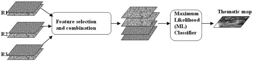
developed by Chen and Stow (2003). The first method is a simple process, which

involves selection of features at all the resolution levels and applying the classification

scheme to obtain the class maps (Figure 1.3). The second is a simple, but very effective bottom-up technique for integration of image classification maps at multiple spatial

resolutions. This technique compares the a posteriori probabilities at different spatial

resolutions, after which the class with highest probability is assigned those pixels that

conformed to the probability conditions (Figure 1.4). The third method is a top-down

used when necessary (Figure 1.5). The computation cost in the first method is very high, while with the third method, class decisions may be made in the absence of fine

resolution information (Chen and Stow, 2003). In this study we therefore applied an

approach similar to the second method, in order to combine the coarse spatial resolution

temporal and high spatial resolution instantaneous imagery sets for classification

purposes.

Figure 1.3 Flowchart for the first fusion strategy, which combines layers of images of varying resolution and then classifies them (Chen and Stow, 2003).

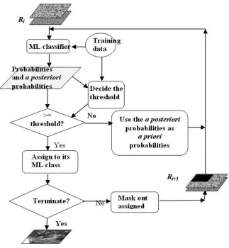
Figure 1.4 Flowchart for the second strategy on combination of various spatial resolutions (Chen and Stow, 2003). This is a bottom-up approach where pixels are assigned to the class with highest posteriori

1.4.

Hypothesis and Objectives

The in-depth literature review and associated outcomes from past studies have led

to the development of the main hypothesis that land cover classification results can be

improved in terms of overall and class-level accuracy through the fusion of coarse

resolution time-series imagery and a high resolution multi-spectral image. This study

has the associated three main objectives:

1) Assess the utility of coarse spatial resolution multi-temporal MODIS satellite

imagery for accurate land cover classification;

2) Evaluate the classification efficacy of a fusion-based approach by integrating the

classification maps from the multi-temporal analysis and a single date, high

spatial resolution multispectral image classification; and

3) Determine if land cover information products, to mainly map agriculture lands in

Chapter 2

Methodology

This chapter describes the methodology used throughout the complete algorithm

workflow, from time series classification to fusion of coarse spatial resolution time series

outputs and high spatial resolution imagery classification. Firstly, we summarize the

study area and list the data specification for the MODIS and RapidEye imagery used. The

process starts by performing pre-processing on images from both remote sensing

modalities. This is followed by the time series feature extraction and classification of the

coarse spatial resolution MODIS images. Next, the high resolution multispectral single

date RapidEye image is classified. Finally, a probability-based fusion is performed using

the classification results from the two disparate modality methods, in order to generate

land cover maps at high spatial resolution, while retaining the spatial, spectral, or

temporal benefits from both the image sources in the final classification results. An error

analysis is performed on the final classification results using the 2010 Cropland Data

Layer Product from the U.S. Department of Agriculture and National Agricultural

2.1.

Study Area

Data from the MODIS Terra sensor were used for time-series analysis. The

MODIS 250m Level-3 product (MOD13Q1) is comprised of the vegetation indices-

NDVI and EVI, along with spectral bands for blue, red, near-infrared, and mid-wave

infrared wavelengths (see Table 2.1). All the images are composited at 16-day intervals. The spectral and vegetation indices products were constructed from atmospherically

corrected bi-directional surface reflectance. Time series of all the images were generated

for five years, from July of 2005 to July of 2010, with each year contributing 23 images.

In addition to this, two mosaicked high spatial resolution RapidEye images (5m),

acquired in July of 2010, were used as a second source of data for the fusion approach.

The MODIS and RapidEye images covered the area surrounding the Nine Mile

Point Nuclear Power Plant in Oswego, NY. This region is diverse in terms of the number

of crop types that are present. According to the Cropland Data Layer Product from the

U.S. Department of Agriculture and National Agricultural Statistics Service, generated in

2010, the study area boasts 58 crop types. In addition, there are vast land areas of

woodlands, wetlands, shrub lands, and barren lands; moreover, a section of Lake Ontario

was also a part of the image used. In terms of crops types, the acreage was dominated by

Hay, Corn, Pasture grass, Soybeans and Fallow or Idle croplands. The images also

covered large portions of urban areas with the towns of Oswego, Fulton, and northern

parts of Syracuse. Validation of classification results was performed using the 2010

specific crop types, at a spatial resolution of 30m (USDA-NASS, Cropland Data Layer

Product, 2010). For validation purposes, this was re-sampled to the same spatial

resolutions as the MODIS and RapidEye datasets.

2.2.

Imagery Specifications

Table 2.1 lists the specifications for the MODIS and RapidEye images.

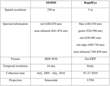
Table 2.1 Data specifications for the MODIS and RapidEye imagery.

MODIS RapidEye

Spatial resolution 250 m 5 m

Spectral information red (620-670 nm)

near-infrared (841-876 nm)

blue (440-510 nm)

green (520-590 nm)

red (630-685 nm)

red edge (690-730 nm)

near-infrared (760-850 nm)

Format HDF-EOS GeoTIFF

Temporal resolution 16-day Daily

Collection time July, 2005 - July, 2010 07-27-2010

Projection Sinusoidal UTM

2.3.

Data Preprocessing

Preprocessing constituted a critical step before any useful information could be

extracted from the images. This processing was performed on both image sources,

MODIS data were originally obtained in the sinusoidal projection and therefore required

a re-projection step into the UTM projection to ensure proper alignment with the

RapidEye images. The re-projected data were spatially subset to the same extent as the

RapidEye image, but the edges of the images were extended by a one-sided linear

dimension of the minimum mapping unit (MMU). The MMU is the size of the smallest

feature that can be distinguished at any particular spatial resolution. Improper definition

of the MMU could lead to biased or underestimation of land cover classes (Saura, 2002).

A MMU of 50 hectares was used, given the MODIS spatial resolution of 250m, in order

to avoid any erroneous classifications at the edges (Herald, 2009). The image data were

also converted from the HDF-EOS format to the GeoTIFF format, which is a more

widely accepted image format among software suites. The MODIS Reprojection Tool

(MRTWeb 2.0) was used for re-projection, subsetting, and conversion of the dataset. The

MRTWeb is an open source tool for the MODIS data processing and analysis.

On the other hand, RapidEye data were converted from digital numbers to

top-of-atmosphere reflectance values (see equation 2.1) (Naughton et al., 2011). The Digital

Number (DN) of a pixel was converted into radiance by multiplying each DN by the

radiometric scale factor.

(2.1)

where, i is the number of the spectral bands, REF is the reflectance value, RAD is the

units, EAI is the Exo-atmospheric irradiance, and SolarZenith is the solar zenith angle in

degrees (=900 – sun elevation). For RapidEye the EAI values for the 5 bands are 1997.8

W/m2μm (blue), 1863.5 W/m2μm (green), 1560.4 W/m2μm (red), 1395.0 W/m2μm (red

edge), and 1124.4 W/m2μm (near-infrared).

In addition to the above conversion, cloud detection was performed on the

RapidEye imagery with an obvious expectation of improvement in classification

accuracies. This was done using a band threshold analysis on the red spectrum. The cloud

pixels were detected by comparing the DN values with a threshold value for the red band

(Naughton et al., 2011). The threshold value, as estimated using trial and error method,

was 17,500 units in digital numbers. The threshold method had numerous disadvantages,

such as inability to detect haze, or “darker” or “small” clouds; moreover, bright features

such as snow, ice or desert sand may be incorrectly classified as clouds. Despite these

limitations, the cloud detection results were visually accurate and this method was used

for its simplicity and low computational requirements. It is obvious that, should this

processing workflow be adopted in future, the user would need to perform an interactive

cloud removal via this or a similar procedure.

2.4.

Time Series Classification

The MODIS time series images were used for obtaining classification maps at a

coarser spatial resolution, but higher temporal resolution (approximately bi-weekly). Four

the MODIS imagery. The pre-processing steps were performed to obtain corrected

reflectance images, i.e., atmospherically corrected bi-directional surface reflectance that

have been masked for water, clouds, heavy aerosols, and cloud shadows, which were

used directly after processing with MRTWeb.

Apart from the spectral bands, vegetation indices were also extracted to enhance

the accuracy (broader class inclusion) and utility (defining vegetation classes) of the

classification. The normalized vegetation index (NDVI) is the most commonly used

vegetation index, used to represent photosynthetic activity or “greenness” in any form of

vegetation. However, it has limitations such as being sensitive to within-pixel soil surface

exposure and loss of sensitivity in presence of high cover or dense canopies (Huete et al.,

2002). Other indices, such as the enhanced vegetation index (EVI) and Soil Adjusted

Vegetation Index (SAVI) were evaluated in order to overcome these limitations. EVI

addresses the drawbacks of NDVI and also provides some additional advantages, such as

correcting for canopy background signals, reducing the influence of atmospheric

conditions on vegetation index values, and increasing the spectral sensitivity in areas with

high biomass density. SAVI and Modified Soil Adjusted Vegetation Index 2 (MSAVI2),

on the other hand, address the issues that NDVI has with areas with low vegetative cover

and with sub-pixel exposed soil surfaces (Terrill, 1994). The entire set of vegetation

indices therefore presents a variety of metrics and provides an extensive range of spectral

information, while performing well for nearly all types of vegetation cover (Huete et al.,



(2.2)

 _(2.3)



(2.4)

 _(2.5)

where, NIR is the near-infrared spectral reflectance, RED is the red spectral reflectance,

BLUE is the blue spectral reflectance, L is the canopy background adjustment (L=1), and

C1 and C2 are coefficients of the aerosol resistance term that uses the 500nm blue band of

MODIS (Huete et al., 1999).

The list of spectral bands and vegetation indices, used as input for time-series

classification, included blue, red, near-infrared, and mid-infrared reflectances, as well as

NDVI, EVI, SAVI, and MSAVI2 as indices. Each of the spectral bands and vegetation

index data were organized in the form of a stack (Figure 2.3), where each 250m x 250m pixel from this stack would represent the temporal profile of that pixel. This temporal

stack is analogous to a hyperspectral image, where the third dimension represents “time",

Figure 2.3 Representation of a "temporal stack" of MODIS imagery, where the temporal dimension for a pixel at a specific wavelength or index is represented in the third dimension.

Figure 2.4 An example of a MODIS “hyper-temporal” red reflectance curve (shown for the pixel indicated on the left RGB image). The third dimension or the band number represents a time period of five years with

a 16-day resolution.

Another important observation with MODIS is the large size of the ground sample

distance, where a typical pixel contains a mixture of different land cover types; an

involves fusion of such pixels with considerably smaller size pixels, e.g., the resolution

ratio between MODIS and RapidEye images is 50. This spatial complexity often is

exacerbated by spectral challenges, e.g., mixed pixels, different scattering properties of

sub-pixel materials, etc.

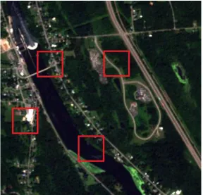
Figure 2.5 An example of a RapidEye scene marked with MODIS pixel size blocks. Mixture of different land classes can be observed in MODIS pixels.

When working with time series data, the default corrections performed on the

MODIS products are often not sufficient. This is because of atmospheric and seasonal

variations over time, which cannot be corrected for with individual images. Such an

present in the temporal curves (curves shown in the results section Figure 3.1). Savitzky-Golay smoothing (Jönsson and Eklundh, 2004) therefore was applied to filter the

temporal curves for these signal spikes. This filter approximates the function within a

moving window by a polynomial of higher degree. All data values are replaced by a

linear combination of nearby values in a window. The filter can be expressed

mathematically as equation 2.6.

(2.6)

where, Ii, i=1, 2, … represent the data values and c = 1 / (2n+1) are the weights for a

moving average filter, in the simplest case. The data value, Ii, is replaced by the average

of the values in the window. In order to avoid losing any critical time series features from

the curves, the temporal resolution of the window size was kept to less than two months

in temporal units. Smoothened temporal curves were obtained after the filtering, which

were used as inputs to the next steps in the processing chain (smoothing results presented

in the results chapter). The data were now ready for classification analysis.

The basic assumption, as required by any classification based on time-series data,

was that different land cover types exhibit unique temporal signatures over time. For the

purpose of distinguishing the maximum number of classes, seven categories - forest,

agriculture, urban, barren, water, wetlands, and shrub lands - were formed (Anderson et

al., 1976). However, it was observed that wetlands, along with shrub lands, exhibited a

behavior very similar to the agricultural lands, whereas the time profiles of barren lands

resembled either urban or agricultural pixels. After a thorough inspection of temporal

coarse resolution MODIS data (Table 2.2). The temporal profiles for these four land-cover types for all the different vegetation indices can be seen in Figure 2.6 - Figure 2.9. It should be noted that though these curves were generated using manually selected pure pixels;

however, a certain level of impurity, due to mixture of classes within these pixels, should

be expected in the case of most pixels, especially those with a low spatial resolution. For

example, the urban category pixels had areas with trees and other vegetation cover.

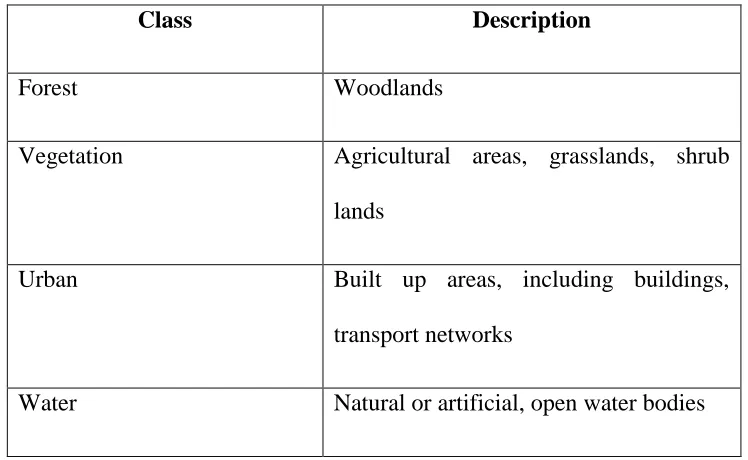
Table 2.2 Description of the final four land cover types used in the classification algorithm.

Class Description

Forest Woodlands

Vegetation Agricultural areas, grasslands, shrub

lands

Urban Built up areas, including buildings,

transport networks

Figure 2.6 Smoothed Normalized Difference Vegetation Index (NDVI) temporal profiles for the four classes.

Figure 2.8 Smoothed Soil Adjusted Vegetation Index (SAVI) temporal profiles for the four classes.

2.4.1 Time Series Feature Metric Extraction

Six features were calculated using the temporal curves for each spectral band and

vegetation index to characterize the phenological differences among the classes (Table 2.3); these features subsequently were used as inputs to the classification. Distinct profiles

for the classes hinted at typical, class-specific attributes that could be exploited, while

these features also were quantified. For example, some of these observations with EVI

profiles (Figure 2.10) were that (a) forested lands have higher crest or “summer peak” values than other vegetation types, ascribed to the denser canopy cover, (b) vegetation

and urban cover have lower trough or “winter dip” values, as opposed to agriculture and

forested lands which typically do not exhibit exposed bare soil and snow during winter,

and (c) EVI values for water were more distinct (flatter) and fluctuated closer to zero.

Similar conclusions were drawn from other temporal profiles. These observations,

supported by the conclusions from Zhang et al. (2008), assisted in the derivation of a

credible set of time-series pixel-based features or metrics for land cover classification.

Table 2.3 Time series feature metrics computed using the temporal profiles.

Feature name Definition

Mean Mean time-series value

Max Maximum time-series value (at crests)

Feature name Definition

Peak-to-peak Difference of the maximum and minimum

values

Winter cycle Approximated by the length between the

negative to positive inflection points

(during troughs) in time-series

Summer cycle Approximated by the length between the

positive to negative inflection points

(during crests) in time-series

Figure 2.10 EVI time series curves for four land cover classes after Savitzky-Golay smoothing. A number of distinct features were observed, e.g., peak-to-peak values for the forest class was high, while urban and

The temporal stacks were comprised of 23 images per year for five years, which

results in a total of 115 images for each feature. The six time-series metrics were

computed for all eight spectral bands and vegetation indices, thus resulting in a total of 48

features. The time-series-based feature calculation effectively reduced the data

dimensionality, i.e., the number of bands for each spectral band and vegetation index,

from 115 to just six. Still, the reduced data set is expected to have some redundancy,

mainly due to the similarity in temporal behavior of different spectral bands and

vegetation indices. Therefore, as a second iteration of data mining, namely stepwise

discriminant analysis, was used to reduce these 48 metrics to approximately ten, a

number which conforms to other classification studies that are based on high dimensional

data (van Aardt et al., 2001). Stepwise discriminant analysis reduces the data set to those

variables that maximize between statistical group variability while minimizing within

group variability, for a given α-level. This was done using the “PROC STEPDISC”

function from SAS 9.3. The significance level (α-level) for assessing which variables

were useful for class separation was kept at 0.01 or 1%.

2.4.2 Classification Metrics

Two distance metrics were used as measures for classification – the Euclidean and

Mahalanobis distances. The Euclidean distance (D) between two points in the spectral

(2.7)

where, x is the coordinate of any unknown pixel and m is the mean vector of a class in the

spectral space. Whereas, the Mahalanobis distance (d) is defined as

_(2.8)

where, x is any unknown pixel in space, m is the mean vector for each class, and S is the

covariance matrix for the same class. More detailed descriptions for these measures can

be found in Schott (2007). A library comprised of pure pixels for each land cover type,

was used as training and validation data. These data accounted for approximately 1% of

the total pixels in the image, and were deemed sufficient (Gupta and Rajan, 2010).

Certain conclusions by Congalton (1991) were used for selecting the training and testing

samples. A minimum number of 100 samples for each category was collected, since the

study area has a large number of vegetation types. For both the coarse and high spatial

resolution approaches, the training data were comprised of spatially diverse regions with

sample clusters not greater than 10 pixels in size.

Using the distance metrics, probability maps were generated for all the pixels as

members of any of the four classes. The probability maps were converted to a posteriori

probabilities of class membership, which could be assessed as probability densities for

the classes (Chen and Stow, 2003). The classification map was converted into a

posteriori probabilities using the equation

where, P( is the probability for a pixel k as a member of class i, is the a priori

probability of membership of class i, and n is the total number of classes. The classes

were assumed to have equal a priori probabilities during this calculation.

2.5.

High Spatial Resolution Classification (RapidEye)

The next step in the process was the classification of a single date, multispectral,

high spatial resolution image, which theoretically should be acquired closely following a

disaster event. Although there is a significant difference in the spatial resolution between

MODIS and RapidEye imagery, the classification methodology for the high spatial

resolution image was kept similar to the coarse resolution MODIS imagery. The

cloud-masked reflectance image was classified using the Euclidean and the Mahalanobis

distance metrics. The training and validation data sets were prepared using the ENVI

Region of Interest (ROI) tool. The classification then were converted into class

probability maps and further transformed into a posteriori probabilities. Unlike the coarse

spatial resolution MODIS imagery, the multispectral image had the potential to

distinguish grass from crop cover. However, since the results from this approach were to

be fused with the coarse resolution results, such classes were merged into similar

2.6.

The Fusion Method

The final and most crucial step in the workflow was the fusion of the class

probability maps from high spatial and coarse spatial, but high temporal resolution

images. A bottom-up strategy was used for the integration of classification results. In this

method, a comparison of the a posteriori probabilities was performed for all four classes

at each high spatial resolution pixel. The coarse spatial resolution probability maps were

sampled to higher resolution for ease of comparison. An added advantage with this

re-sampling was generation of the final classification results at higher spatial resolution. The

probabilities can be regarded as a measure of confidence with which the classification has

assigned a pixel to a given class.

The sum of class probabilities for each pixel should equal 1.0, once the

classification maps are transformed into probabilities. At both the spatial resolutions, the

higher probability and the corresponding classes were recorded for each pixel.

represents the maximum a posteriori probability of a pixel k belonging to class i at

resolution level l. is derived from all resolutions, and k is assigned to the class

with the highest a posteriori probability. Thus, k would belong to class c if, and only if,

_(2.10)

where, i = 1, 2, 3, …, m possible classes, l = 4m, 8m,…, possible resolutions. In

accordance with our implementation, the pixels were assigned to the class with the higher

2.7.

Error Analysis

Error analysis was performed to validate the classification scheme. The final land

cover maps were compared to the test/validation dataset generated from the 30m spatial

resolution USDA Cropland Data Layer Product (USDA-NASS, Cropland Data Layer

Product, 2010). This dataset has 58 agricultural and six non-agricultural classes, which

were combined in order to obtain the same four exhaustive classes used in the

classification. For the validation of the coarse resolution class maps, the validation

dataset was re-sampled from 30m to 250m, whereas fusion results were re-sampled from

5m to 30m for comparison. For both of these resolutions, re-sampling was performed

using the nearest neighbor technique (Schott, 2007).

In addition to re-sampling, the improper registration between the class maps and

the validation dataset presented another challenge while comparing the fusion class maps.

There was clearly an impact of re-sampling on validation, particularly across the 50 times

change in spatial resolution. A pixel-to-pixel comparison would be a simple, but a

restrictive way for evaluating the class maps. An alternative scheme was established to

take into account a spatial generalization. Since the class maps being tested consisted of

information from both the low, as well as high spatial resolution data, errors attributable

to mis-registration or inability to confidently photo-interpret a sample unit would be

large. Therefore, a definition of agreement was developed between the class map and the

ground truth maps. A sample pixel was compared with the most common class within a

generalization can be achieved and mis-registration errors up to one pixel in any direction

Chapter 3

Results and Discussion

The results presented in this section cover classification using (i) coarse spatial

resolution time-series MODIS imagery, (ii) high resolution multi-spectral RapidEye

imagery, and (iii) the high-temporal high-spatial resolution fusion-based approach.

3.1.

Time Series Classification

Pre-processing - time profile smoothing

An example of Savitzky-Golay filtering results for EVI time-profile is shown in

Figure 3.1. It can be observed that the basic time series contour was preserved, while a relatively minimal loss of time series features occurred after smoothing the curves. The

smoothened temporal curves, obtained after filtering, were used to derive input features

for the subsequent classification steps. This was based on the conclusion that the

temporal trends were conserved, even though fine resolution temporal features may be

lost during this pre-processing step. These high frequency features arguably could

introduce noise during the classification steps, given that such fine temporal occurrences

are often due to intra-annual anomalies. The sharp decrease of the time-series curves in

the fall and sharp increase in the spring can be attributed to snowmelt and snow

Figure 3.1 An EVI time series for a typical vegetation cover pixel, before and after the Savitzky-Golay smoothing, to filter high frequency spikes